Munich Personal RePEc Archive
Procrastination, self-imposed deadlines
and other commitment devices
Bisin, Alberto and Hyndman, Kyle
Southern Methodist University
16 March 2009
Online at
https://mpra.ub.uni-muenchen.de/16235/
Procrastination, Self-Imposed Deadlines and Other
Commitment Devices
Alberto Bisin
∗New York University
Kyle Hyndman
†Southern Methodist University
March 16, 2009
Preliminary and Incomplete
Abstract
In this paper we model a decision maker who must exert costly effort to complete a single task by a fixed deadline. Effort costs evolve stochastically in continuous time. The decision maker will then optimally wait to exert effort until costs are less than a given threshold, the solution to an optimal stopping time problem. We derive the solution to this model for three cases: (1) time consistent decision makers, (2) na¨ıve hyperbolic discounters and (3) sophisticated hyperbolic discounters. Sophisticated hy-perbolic discounters behaveas if they were time consistent but instead have a smaller reward for completing the task. We show that sophisticated decision makers will often self-impose a deadline to ensure early completion of the task. Other forms of commit-ment are also discussed.
∗Department of Economics, New York University, 19 W 4th
Street, 6th
Floor, New York, NY 10012. E-mail: [email protected], url: http://www.econ.nyu.edu/user/bisina.
1
Introduction
People seem to tend to procrastinate in many matters, including some with significant eco-nomic consequences. This behavior could be due to a form of time inconsistency of pref-erences (e.g., a preference for the present as represented by hyperbolic or quasi-hyperbolic discounting; see Phelps and Pollak (1968), Laibson (1994, 1997) and O’Donahue and Rabin (1999a,b)). However, this behavior could also represent, an optimal decision to “wait for better times” in an environment in which acting requires the exertion of costs which evolve stochastically over time. To better distinguish between these two motivations for procras-tination, in this paper we study the decision problem faced by a single decision maker who has to decide if and when complete a task before some fixed, final deadline that provides a delayed benefit but requires the immediate exertion of effort. We study the case where effort is costly and evolves according to a continuous time stochastic process, and the agents preferences are either time consistent or are characterized by quasi-hyperbolic discounting.
When agents have standard, time-conistent, preferences our model is formally equivalent to the exercise of an American put option. In particular, we show that the decision maker adopts a threshold rule. That is, at each time t, there is a threshold cost, such that if the realized cost of effort at timetis below the threshold, the agent completes the task; otherwise, she waits. The threshold cost increases as the agent gets closer to the final deadline. That is, for the same realized cost, the agent if less likely to delay the closer she is to the final deadline.
In order to study the behavior of decision makers with a present bias, we adapt the model of Harris and Laibson (2004) — an elegant generalization of the standardβ−δ quasi-hyperbolic model of Phelps and Pollak (1968) and Laibson (1994) to continuous time. Deci-sion makers can either be na¨ıve or sophisticated (see, e.g., O’Donahue and Rabin (1999b)). Na¨ıve decision makers are unaware of their self-control problems, while sophisticates are aware that they have a tendency to procrastinate. We first show that na¨ıve decision makers will never complete a task strictly before the final deadline. On the other hand, we show that a sophisticated decision maker behaves as if she were an exponential discounter but faced a smaller value to completing the task. That is, the sophisticated agent adopts a threshold which is increasing as she gets closer to the final deadline.
makers will sometimes, optimally, self-impose a deadline strictly more binding than the exogenous final deadline that we impose.
Our paper is related to S´aez-Mart´ı and Sj¨ogren (2008) who study how deadlines affect the timing of effort when agents get distracted (i.e., face a higher cost of effort at certain times). While we focus on continuous time stopping problems, their model is in discrete time, and agents must exert effort in more than one time period. Therefore, it may be that agents start a task but fail to complete it. Another difference is that while they focus on incentives (i.e., deadlines) imposed by principals, we examine whether there is a beneficial role for self-imposed deadlines. One surprising result from their analysis is that agents who are often distracted may outperform agents who are less frequently distracted. This follows because agents who are often distracted exert “precautionary” effort earlier (see ? for some
experimental evidence on this point).
Our paper is also closely related to Hsiaw (2008) who studies the role of self-imposed, though non-binding, goals as a source of motivation for agents with a present bias. Like us,?
adopts the continuous time quasi-hyperbolic model of Harris and Laibson (2004), though the decision makers in her model face an infinite horizon stopping problem, while our agents face some finite deadline. In her model, goals serve as a reference point; in particular, agents get utility from consumption and from comparing outcomes to the self-set goal. Hsiaw (2008) shows that self-set goals can help overcome one’s tendency to procrastinate; however, if self-control problems are minimal (or absent), they can actually be detrimental.
The rest of the paper is organised as follows. The next section describes the decision problem faced by a single decision maker: at what point in time, at or before some final deadline, should the decision maker optimally complete a task that provides a delayed benefit but requires the immediate exertion of effort (where effort evolves according to a stochastic process). We then characterize optimal behaviour under various forms of time discounting. As mentioned above, we show that exponential discounters employ a threshold strategy, completing the task at time t if the cost is less than the time t threshold. Borrowing on results from the literature on American options, we show that the threshold is increasing in time, and also characterise other comparative statics. In particular, since the value of the option (to complete the task later) is increasing the further away from the final deadline, we are able to say that exponential discounters would never self-impose a deadline.
for a sophisticate to do so. We show that if the initial cost realization of task completion is known, then she may actually prefer to set a non-trivial deadline. Indeed, the deadline will be sufficiently strict so that she forces herself to complete the task immediately. When the decision maker faces some uncertainty about her initial cost of completing the task, we are unable to analytically solve for the optimal deadline. In Section 3, we conduct a numerical exercise in order to demonstrate that sometimes the decision maker will, in fact, self-impose a non-trivial deadline when there is uncertainty about her initial cost of task completion. Our numerical results would also seem to indicate that if the decision maker self-imposes a deadline, it is an immediate deadline.
In Section4we study commitment via methods other than self-imposed deadlines affects behaviour. Motivated by some experimental results by Trope and Fishbach (2000), we two such alternative commitment devices are: (i) Making a fixed payment conditional upon task completion and (ii) imposing a cost for not completing the task. In the former case, we show that, provided the final deadline is not too far away, a sophisticated hyperbolic discounter may prefer to make the fixed fee conditional upon task completion (doing so increases the likelihood that the task is ultimately completed). However, if the deadline is far away, then the decision maker prefers to take the payment up front since she knows that she is likely to delay excessively. In the latter case, when the time to the final deadline is sufficiently close, imposing a cost for not completing the task has a similar effect as does making a fixed payment conditional on completing the task. However, as the time to the final deadline increases, the expected burden of not completing the task diminishes and it has substantially less commitment power.
While deadlines in the set-up of Section 2 are extremely strict — if the task is not completed at or before the deadline, the entire value disappears — in reality, and also in the experiments of Ariely and Wertenbroch (2002) and the model of O’Donahue and Rabin (1999b), missed deadlines often lead to less sever penalties. Also in Section 4, we examine the case in which a penalty per time period that the task is not completed is imposed. Such an incentive scheme has its benefits and drawbacks. The benefit is that the weaker deadline does not completely destroy the option value of being able to wait for a lower cost of task completion. The main drawback is that the incentives for early task completion are also weaker. Like our previous results, we show that if β is sufficiently high, the sophisticated decision maker chooses a deadline (i.e., a point in time in which the penalty kicks in) sufficiently strict so as to ensure immediate completion.
will behave as if she had exponential time preferences.
In Section 5 we return to the issue of whether a decision maker would ever self-impose a deadline, but instead we examine other models of decision making. Our first result here is to show that a decision maker with self-control problems `a la Gul and Pesendorfer (2001, 2004) would never self-impose a non-trivial deadline. In this section we also discuss Brunnermeier, Papakonstantinou, and Parker (2007) which proposes a model of optimal expectations in which decision makers will both procrastinate and self-impose a deadline. In their model, decision makers consistently underestimate the amount of work required to complete a task, leading to less than optimal initial effort. However, this leads to an anticipatory utility effect: current felicity is boosted because the decision maker anticipates less work in the future. Finally, Section 6provides some concluding remarks and discusses future directions.
2
The Model
A decision maker is faced with a task that needs to be completed by time T. If completed at or before time T, a task will pay a reward of V > 0. If the task is completed after its deadline no reward will be given. We assume that there is some delay in the payment upon completion of the task. That is, if the task is completed at time t, then the payment V is made at time t+ ∆, where ∆ >0 is a constant. This will not make a much difference for decision makers who exhibit exponential discounting; however, for hyperbolic discounters it creates a small time wedge between when costs are incurred and the rewards are received. Hence, such decision makers will exhibit a tendency to procrastinate.
Suppose also that the cost, x, of completing the a task follows a geometric Brownian motion. That is:
dx=σx·dz (1)
where the parameter σ > 0 captures variance in the obvious way.1 We now proceed to the
write down the general case for an exponential discounter. Later we will formulate and solve the problem of a hyperbolic discounter.
2.1
The Exponential Case
Let W(x, t) = sup0≤τ≤T−tEx,t(e−ρτmax{V¯ −x,0}) denote the value of the task when the
current cost is x, the current time is t (so that time to the deadline is δ := T −t) and ¯
V :=e−ρ∆V. The parameterρ >0 captures the time preferences of the decision maker.
1
This basic problem is formally equivalent to an American put option where the strike price is ¯V and the current price of the underlying security is x(t). Therefore, all of the tools and results derived from this literature will guide us here. In particular, it is well known that the solution to this problem leads to a threshold function ¯x(t), such that for x(t)≤x¯(t) the decision maker will complete the task, while when the opposite inequality holds, the agent prefers to wait. Moreover, it is well known that in the continuation region W(x, t) is the solution to the following free boundary problem:2
ρW(x, t) = 1 2σ
2x2W
xx(x, t) +Wt(x, t) (2)
W(¯x(t), t) = ¯V −x¯(t) (3)
Wx(¯x(t), t) = −1 (4)
W(x,0) = max{V¯ −x,0} (5)
In the language of Dixit and Pindyck (1994), (3) represents the value matching condition and the threshold, while (4) is the smooth pasting condition at the boundary and (5) is the terminal condition describing optimal behaviour at the deadline.
2.1.1 Comparative Statics
The solution to this problem does not admit an explicit, closed form solution and one must instead rely on numerical techniques or analytic approximations. However, many properties of the value function and the threshold cost function are known. The most important from our perspective being the properties of the equilibrium threshold function, ¯x(t) and also the deadline. We now prove a few results and also provide some intuition for them. An intuitive discussion can be found in Hull (2005), while Peskir and Shiryaev (2006) contains an advanced treatment.
¯
x′(t)≥0. That is, the threshold cost realisation is increasing in time. That this is so is
quite intuitive. As one approaches the deadline, there is less time remaining during which one can wait for lower cost realisations to materialise. More formally:
Proposition 1. The optimal threshold, x¯(t) is increasing in t.
Proof. Notice that the gain function max{V¯ −x,0} does not depend on time. Therefore, we may conclude that W(x, t) is decreasing in t for each x ∈ R++. Suppose that x > x¯(t)
for some t so that W(x, t)−max{V¯ −x,0} > 0. Now take any t′ ∈ [0, t). It follows that
2
W(x, t′)−max{V¯ −x,0} ≥ W(x, t)−max{V¯ −x,0} > 0, which implies that x > x¯(t′),
which in turn implies that ¯x(t) is increasing int.
The effect of ρ is ambiguous. Observe that an increase in ρ has a negative effect on the option value of waiting, which all else equal, would increase the threshold cost realisation (see, in particular, Peskir and Shiryaev (2006)). However, since the reward, ¯V =e−ρ∆V, it
is also true that an increase inρlowers the reward from completing the task, and it is known that ¯x(t) is increasing in the reward. Therefore, these two effects go in opposite directions and the total effect of an increase in ρ cannot be conclusively determined.
∂¯x
∂σ <0. The higher is volatility, the more likely it is that there will be wide swings in
the cost of task completion. Moreover, as is standard, the decision maker is shielded from cost increases (he can always not exercise the option) and benefits from cost decreases. We formally state, but do not prove, the following:
Proposition 2. The optimal threshold, x¯(t) is decreasing in σ.
2.1.2 The Optimal Deadline
Here we show that the decision maker prefers a later deadline to an earlier one. Letωτ denote
the optimal policy given a deadline ofτ and letWτ(x, t;ω
τ) denote the value obtained by the
decision maker at time t with initial cost realisation x, facing a deadline of τ and following the optimal policy. With this notation, we are now ready to demonstrate:
Proposition 3. An exponential discounter prefers later to earlier deadlines.
Proof. Consider two different decision problems, differentiated only by their deadlines. As-sume that τ < τ′. We know that Wτ′
(x, t;ωτ′) ≥ Wτ ′
(x, t;ωτ) ≥ Wτ(x, t;ωτ). The first
inequality comes from the optimality of the policy ωτ′ when faced with deadline τ′. The
latter inequality comes from the fact that exactly the same outcomes arise since the same policy is being implemented in the two situations; however, in the former case, the accumu-lated rewards from completing tasks are weakly higher because τ′ > τ. Therefore, we have
shown that the decision maker prefers later deadlines to earlier ones.
2.2
The Hyperbolic Case
but are themselves unaware of it. That is, in period t, she discounts future flows according to βγ, βγ2, . . .; however, importantly, she assumes that next period she will behave as an
exponential discounter would. This type of behaviour has been shown to create substantial amounts of procrastination. On the other hand, sophisticated decision makers recognise that they are time inconsistent. Therefore, the decision problem is often modelled as a dynamic game with different versions of one’s self at each period. In this way, a sophisticate anticipates what her future self will actually chose, but still discounts according to βγ. Generally speaking, it is substantially more difficult to characterise optimal behaviour for sophisticates than for na¨ıfs or even exponential discounters.
Our discussion of hyperbolic discounting will be divided into two parts: an analysis of na¨ıfs and sophisticates. In both cases, we will adopt the framework of Harris and Laibson (2004) in order to model hyperbolic discounting in continuous time. In particular, a decision maker born at time t can be divided into twoselves: the present self, lasting fromt tot+ג,
and the future self, lasting fromt+גto∞. The length of time that the present self exercises
control is then ג, which is stochastic and, as in Harris and Laibson (2004), is exponentially
distributed with parameter λ ≥0. The discount function of a decision maker born at time 0 can then be summarised as follows:
D(t) = (
γt if t ∈[0,ג)
βγt if t ∈[ג,∞)
where γ ∈(0,1) and β ∈(0,1]. For ease of notation, define ρ=−lnγ.
2.2.1 Naïve Decision Makers
We first consider a na¨ıve decision maker. As with the exponential case above, there will be a threshold cost realisation below which it is optimal to complete the task, and above which it is optimal to wait. Let Wn(x, t) denote the value function of a na¨ıf and We(x, t) denote
the value function of the exponential discounter. For any pair (x, t), in an interval of length
dt, the value function, Wn(x, t), must solve:
Wn(x, t) = max{U(λ)−x , e−ρdtE
e−λdtWn(x+dx, t+dt)
+(1−e−λdt)βWe(x+dx, t+dt) (6)
where U(λ) =e−λ∆V¯ + (1−e−λ∆)βV¯ is the expected discounted payment from completing
the task immediately.3 If the decision maker transforms into her future self, which occurs
3
with probability 1− e−λdt, then she discounts the future by the extra factor β, but she
anticipates that she will behave as the exponential discounter would — hence our inclusion of We(x+dx, t+dt).
Now suppose that we are in the region for which it is optimal to wait. Multiply both sides of (6) by eρdt and subtract Wn(x, t) to obtain:
(eρdt−1)Wn(x, t) = e−λdtE
[Wn(x+dx, t+dt)−Wn(x, t)]
+ (1−e−λdt)E[βWe(x+dx, t+dt)−Wn(x, t)]
which, upon noting that eρdt ≈1 +ρdt, e−λdt≈ 1−λdt and applying Ito’s Lemma, can be
simplified to:
ρdtWn(x, t) = (1−λdt)E[Wn
xdx+
1 2W
n
xxdx2+Wtndt]
+ λdt[βWe(x+dx, t+dt)−Wn(x+dx, t+dt)]
Diving through by dt and taking the limit as dt→0, we arrive at:
ρWn(x, t) = 1 2σ
2x2Wn
xx(x, t) +W n
t (x, t) +λ[βW
e(x, t)−Wn(x, t)] (7)
along with the following optimality conditions:
Wn(¯xn(t), t) = U(λ)−x¯n(t) (8)
Wxn(¯xn(t), t) = −1 (9)
Wn(x, T) = max{U(λ)−x,0} (10)
It is intuitively obvious that ¯xn(t) ≤x¯e(t) for all t and for all λ >0. This is so for two
reasons. First, the reward, U(λ) ≤ V¯. Therefore, there are simply fewer cost realisations for which the na¨ıve decision maker can profitably complete the task. Second, for all λ >0, there is always a positive probability that the current self will relinquish control over task completion to her future self. Importantly, however, the current self believes that her future self will behave as an exponential discounter would. This means that she believes that her future self will be more likely to complete the task, making waiting optimal.
An interesting thing happens in the limit as λ → ∞; namely, Wn(x, t) = βWe(x, t) in
the waiting region for the na¨ıve decision maker. That is,
Wn(x, t) = max{βV¯ −x, βWe(x, t)}
we claim that the decision maker will never complete the task for x(t) > 0 and t < T. Take any 0 < x(t) ≤ x¯e(t), so that the exponential discounter would rationally choose to
complete the task. Therefore, the hyperbolic discounter will complete the task if and only if
x(t)≤β[ ¯V −( ¯V −x(t))] =βx(t). Since β <1, this can only be satisfied provided x(t) = 0. Therefore, as λ → ∞, it becomes ever less likely that the na¨ıve hyperbolic discounter will complete the task at any time t < T and will complete the task at time T if and only if
x(T)≤βV¯. Formally, we have:
Proposition 4. Unlessx(t) = 0, the na¨ıve decision maker will complete the task only at time
T and only if x(T)≤βV¯.
2.2.2 Sophisticated Decision Makers
We now turn our attention to sophisticated decision makers. The approach we take is similar to that of the previous subsection, though there are a few conceptual differences brought on by sophistication. In particular, the current self anticipates the actions that will be taken by her future self and incorporates these decisions into the current value function. Therefore, we can define a current value function Ws(x, t) (“s” for sophisticated) and a continuation
value function wc(x, t) (“c” for continuation).
As with the previous cases, there will be a threshold cost ¯xs(t) below which it is optimal
to complete the task, and above which it is optimal to wait. In the waiting region, it is not difficult to see that the continuation value function can be expressed the following partial differential equation:
ρwc(x, t) = 1 2σ
2x2wc
xx(x, t) +w c
t(x, t) (11)
which has the same form as in (2), but does not also come explicitly endowed with boundary conditions, nor value-matching or smooth-pasting conditions. This is becausewc is not being maximised, but is instead being evaluated according to the policy function for Ws, which we now seek to derive. Outside of the waiting region, we also have wc(x, t) = ¯V −x.
Consider now Ws(x, t). It may be expressed as:
Ws(x, t) = max{U(λ)−x , e−ρdtE
e−λdtWs(x+dx, t+dt)
+(1−e−λdt)βwc(x+dx, t+dt) (12)
Running through the same steps as for the na¨ıve hyperbolic discounter, we are able to re-write (12) in the waiting region as:
ρWs(x, t) = 1 2σ
2x2Ws
xx(x, t) +W s
t(x, t) +λ[βw c
Of course, optimality requires the following extra conditions:
Ws(¯xs(t), t) = U(λ)−x¯s(t) (14)
Wxs(¯xs(t), t) = −1 (15)
Ws(x, T) = max{U(λ)−x,0} (16)
Therefore, for each λ > 0, the equilibrium solution for the hyperbolic discounter is given by a solution to (11) and (13) – (16). Note also that as λ → ∞, we have that
βwc(x, t) = Ws(x, t) in the waiting region. In fact, this key insight allows us to fully
char-acterise the solution. Since wc(x, t) satisfies the partial differential equation (11) and since
Ws(x, t) =βwc(x, t), implies thatWs(x, t) must also satisfy (11). That is, Ws(x, t) satisfies:
ρWs(x, t) = 1 2σ
2x2Ws
xx(x, t) +Wts(x, t), which together with the boundary conditions (14)
– (16) is identical to the decision problem faced by an exponential discounter in which the reward for completing the task is βV¯ instead of ¯V. Formally stated,
Proposition 5. In the limit as λ → ∞, the sophisticated hyperbolic discounter behaves as if he were an exponential discounter in which the reward for completing the task is βV¯.
2.2.3 The Optimal Deadline
It is obvious that the na¨ıve decision maker will set the latest possible deadline since she believes as though she will behave like an exponential decision maker in the future, and it was shown in Proposition3that exponential decision makers prefer later deadlines. However, this is not necessarily the case for sophisticated decision makers. They would like their future selves to behave like exponential decision makers but know that they will not. Therefore, since the task is simply a stopping time problem, the only way for the sophisticated decision maker to influence when the task gets completed is to set an earlier deadline.
We begin with the case in which the decision maker knows with certainty what the cost realisation will be at time 0 (i.e.,x(0) is known). We claim the following:
Proposition 6. There exists some initial cost realisation,xˆ, such that ifx(0) ≤xˆ, the decision maker sets any deadline τ such that x(0) ≤x¯s(0, τ). Otherwise, the decision maker sets the longest possible deadline.
Proof. Observe that if the decision maker completes the task at time 0, then her utility is simplyβ(V −x(0)). On the other hand, if she does not immediately complete the task, then her expected utility is βwc(x(0),0;τ). From Proposition 5, we know that βwc(x(0),0;τ) =
Ws(x(0),0;τ) and that Ws is the value function of an exponential decision maker with a
It is also relatively easy to see that as τ → ∞, W(x,0;τ) → Axα for x > x¯(0,∞) = α
α−1βV¯, where α is the negative root of the fundamental quadratic:
σ2
2 α(α−1)−ρ= 0 and
A = −x¯(0,∞α)1−α. Therefore, ˆx is given by the unique solution to Axα = β( ¯V −x). Then,
since the function ¯xs(0, τ) is monotonic in τ, we can invert it to determine ˆτ, where ˆτ is the
weakest deadline such that the decision maker immediately completes the task at time 0. Of course, any deadline τ′ <ˆτ will also ensure immediate completion of the task and would
also represent an optimal decision for x≤xˆ.
The intuition for this would seem to be as follows: since there is a “discontinuous” benefit to completing the task immediately (which arises due to sophistication), the decision maker would like to commit her time 0 self to immediately complete the task. On the other hand, there is still the option value of waiting to complete the task, and this value is increasing in the time to the deadline. Therefore, if it is known that the initial cost will be quite low the discontinuous benefit of commitment outweighs the benefit of holding an option to complete the task at later date, while if it is known that the initial cost will be quite high, then a commitment to immediately complete the task becomes more costly relative to the benefit of holding the option to complete the task at a future date when, possibly, the cost of doing so is lower.
Of course, if there is a significant delay between when the decision maker chooses a deadline and when she may actually begin working on the task, the assumption that she knows x(0) with certainty becomes strained. Therefore, suppose that x(0) is a random variable, the realisation of which is drawn from the distribution function F such that ˆx ∈
supp(F). Intuitively, for realisations x ≤ xˆ, the decision maker would like to set a very strict deadline to ensure immediate completion of the task, while for realisationsx >xˆ, the decision maker prefers no deadline at all. Therefore, by integrating over the support of F, an intermediate deadline may become optimal.
A bit more formally, observe that we may write theex anteexpected utility of the decision maker as follows:
¯
Ws(τ) = Ex[βwc(x,0;τ)] =
Z x¯s(0,τ)
0
β( ¯V −x)dF(x) + Z ∞
¯
xs(0,τ)
βwc(x,0;τ)dF(x) (17)
where τ is the deadline, ¯xs(0, τ) is the optimal threshold at time 0, wc(x,0;τ) denotes the
continuation value of the decision maker. Importantly, notice thatβwc(x,0;τ) = Ws(x,0;τ)
and for x ∈ (¯xs(0, τ),x¯s(0, τ) +ǫ), Ws(x,0;τ) ≈ βV −x < V −x. Notice also that Ws
Leibniz Rule, after some simplifications, we obtain:
∂W¯s(τ)
∂τ = (1−β)¯x
s(0, τ)f(¯xs(0, τ))∂x¯ s
∂τ +
Z ∞
¯
xs(0,τ)
Wτs(x,0;τ)dF(x) (18)
There are two opposing effects at play in the above equation. If τ is increased by a small amount, then the threshold for immediate task completion is lowered. This leads to a utility loss of (1−β)¯xs(τ). On the other hand, by increasing the deadline, the decision maker is
giving herself more opportunities to actually complete the task at some point in the future. Thus she experiences a gain, which is represented by the integral. Therefore, without further assumptions, it is not possible to analytically characterise the stationary points of (18). In order to gain further intuition, we solve for the optimal deadlines numerically in the next section.
3
A Numerical Exercise to Find Optimal
Self-Imposed Deadlines
Given the inability above to formally show whether a sophisticated hyperbolic discounter will set a deadline when there is uncertainty over the initial cost realisation, we seek to answer this question numerically. Our task is greatly facilitated by Proposition 5, since it tells us that we need to solve for the value function of an exponential decision maker with a value of completing the task of βV¯, which amounts to pricing an American put option with strike price βV¯. To do this, we use the binomial tree method of Cox, Ross, and Rubinstein (1979) to solve forP(x, βV , t¯ ) which is the price of an American put option with “asset price” (i.e.,
cost of completing the task), x, “strike price” (i.e., value of completing the task), βV¯, and time until expiration t. Then, the ex ante value of completing the task at time 0 is:
Ws(0, x, τ) = (
P(x, βV , τ¯ ), if x >x¯s(0, τ)
β( ¯V −x), if x≤x¯s(0, τ)
Then, taking expectations over all possible initial values ofx, we have ¯Ws(τ) =R
xW
s(0, x, τ)dF(x).
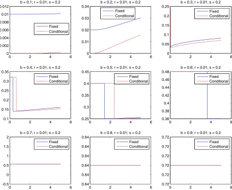
That is, if the decision maker completes the task immediately at time 0, she obtainsβ(V−x), while if she delays at time 0, then her value is the price of the corresponding option. The results of this exercise are shown in Figures 1 – 4. In each figure r and σ are fixed and β
varies from 0.1 to 0.9. On the horizontal axis is the deadline, τ, where τ = 0 represents an immediate deadline and τ = 5 is a deadline of 5 years into the future.
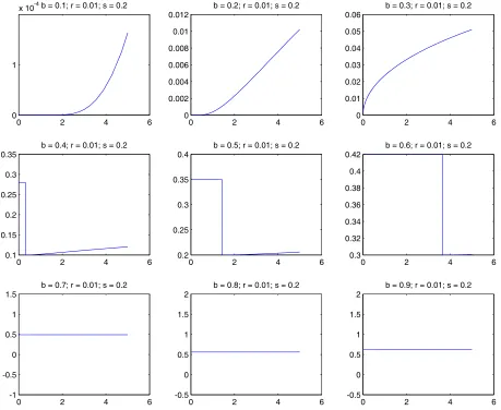
In Figure 1, we conducted the simulation exercise for the case in which the initial cost,
Figure 1: Simulation Results; r= 0.01 & σ = 0.2; x(0) = 0.3, known
0 2 4 6
0 1
x 10-4b = 0.1; r = 0.01; s = 0.2
0 2 4 6
0 0.002 0.004 0.006 0.008 0.01 0.012
b = 0.2; r = 0.01; s = 0.2
0 2 4 6
0 0.01 0.02 0.03 0.04 0.05 0.06
b = 0.3; r = 0.01; s = 0.2
0 2 4 6
0.1 0.15 0.2 0.25 0.3 0.35
b = 0.4; r = 0.01; s = 0.2
0 2 4 6
0.2 0.25 0.3 0.35 0.4
b = 0.5; r = 0.01; s = 0.2
0 2 4 6
0.3 0.32 0.34 0.36 0.38 0.4 0.42
b = 0.6; r = 0.01; s = 0.2
0 2 4 6
-1 -0.5 0 0.5 1 1.5
b = 0.7; r = 0.01; s = 0.2
0 2 4 6
-0.5 0 0.5 1 1.5 2
b = 0.8; r = 0.01; s = 0.2
0 2 4 6
-0.5 0 0.5 1 1.5 2
b = 0.9; r = 0.01; s = 0.2
Proposition6 and also provides further intuition. When β is very low, initially the decision maker prefers an infinite deadline. This follows because an immediate deadline would induce a threshold of βV < x¯ (0), so the ex ante self cannot force his future self to complete the task — hence he prefers no deadline at all. However, as β increases, so that the decision maker’s self control problems become less severe, we see that the he prefers to impose a deadline such that the he immediately completes the task. As can be seen, in general, there exists a threshold deadline τ∗, depending upon the parameters, such that if τ ≤ τ∗,
the task will be completed immediately, leading to a utility of β( ¯V −x(0)) for the ex ante
self. In contrast, for τ > τ∗, ¯xs(0, τ) >0.3, the task is not immediately completed and the
ex ante self experiences a discontinuous drop in his expected value. This follows because
β( ¯V −x(0))> βV¯ −x(0) ≈Ws(x(0),0, τ∗+ǫ). Of course, forτ > τ∗, the ex ante expected
utility (i.e.,Ws(x(0),0, τ)) is increasing inτ. Finally notice that, since ¯xs(0, τ) is increasing
inβ, we also have that τ∗ is increasing in β.
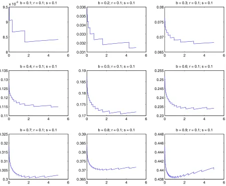
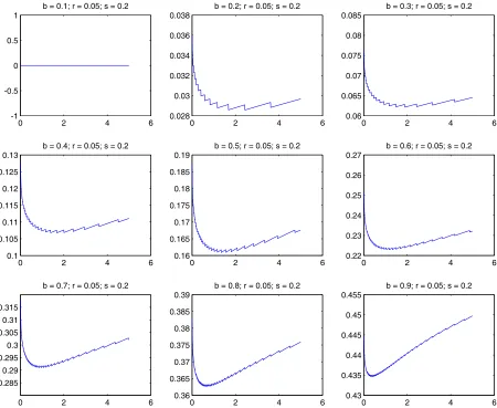
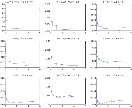
Next turn to Figures 2– 4. These figures provide numerical results for the more realistic case in which x(0) is not known with certainty; in particular x(0) was drawn from the uniform distribution with support [0,1]. As we have discussed above, when x(0) is not known, there is some scope for intermediate deadlines which do not necessarily guarantee immediate task completion. The goal of this exercise is to determine how large that scope is. Notice that the figures appear discontinuous; this is due to the finite grid that was used for the numerical exercise. A finer grid will produce more accurate graphs but at the cost of increased computation time.
Notice that in all cases an immediate deadline provides for a local maximum, with the
ex ante expected value decreasing for very short deadlines. That this is so can be seen by examining once again (18). When τ = 0, Carr, Jarrow, and Myneni (1992) allows us to conclude that ∂¯xs
∂τ =−∞. Therefore, by increasing the deadline even a little bit, theex ante
self is substantially lowering the chance that her future self will immediately complete the task. Therefore, she loses the discontinuous benefit of immediate task completion. However, as τ increases further, ¯xs(τ) becomes flatter and so the loss in the discontinuous benefit of
immediate completion gets mitigated by the increase in option value — the second term in (18). Eventually, especially when β is relatively large this latter effect begins to dominate and ¯Ws(τ) becomes increasing in τ.
Figure 2: Numerical Results; r = 0.05 & σ= 0.1
0 2 4 6
8 8.5 9 9.5x 10
-3 b = 0.1; r = 0.1; s = 0.1
0 2 4 6
0.031 0.032 0.033 0.034 0.035 0.036
b = 0.2; r = 0.1; s = 0.1
0 2 4 6
0.065 0.07 0.075 0.08
b = 0.3; r = 0.1; s = 0.1
0 2 4 6
0.11 0.115 0.12 0.125 0.13 0.135
b = 0.4; r = 0.1; s = 0.1
0 2 4 6
0.17 0.175 0.18 0.185 0.19
b = 0.5; r = 0.1; s = 0.1
0 2 4 6
0.23 0.235 0.24 0.245 0.25 0.255
b = 0.6; r = 0.1; s = 0.1
0 2 4 6
0.3 0.305 0.31 0.315 0.32 0.325
b = 0.7; r = 0.1; s = 0.1
0 2 4 6
0.365 0.37 0.375 0.38 0.385 0.39
b = 0.8; r = 0.1; s = 0.1
0 2 4 6
0.438 0.44 0.442 0.444 0.446 0.448
b = 0.9; r = 0.1; s = 0.1
On the horizontal axis is the deadline; that is, t = 0 represents an immediate deadline, while t = 2 represents a deadline of two years. On the vertical axis is theex ante expected value of the time 0 self.
the decision maker prefers no deadline to an immediate deadline.
Figure 3: Numerical Results; r = 0.05 & σ= 0.2
0 2 4 6
-1 -0.5 0 0.5 1
b = 0.1; r = 0.05; s = 0.2
0 2 4 6
0.028 0.03 0.032 0.034 0.036 0.038
b = 0.2; r = 0.05; s = 0.2
0 2 4 6
0.06 0.065 0.07 0.075 0.08 0.085
b = 0.3; r = 0.05; s = 0.2
0 2 4 6
0.1 0.105 0.11 0.115 0.12 0.125 0.13
b = 0.4; r = 0.05; s = 0.2
0 2 4 6
0.16 0.165 0.17 0.175 0.18 0.185 0.19
b = 0.5; r = 0.05; s = 0.2
0 2 4 6
0.22 0.23 0.24 0.25 0.26 0.27
b = 0.6; r = 0.05; s = 0.2
0 2 4 6
0.285 0.29 0.295 0.3 0.305 0.31 0.315
b = 0.7; r = 0.05; s = 0.2
0 2 4 6
0.36 0.365 0.37 0.375 0.38 0.385 0.39
b = 0.8; r = 0.05; s = 0.2
0 2 4 6
0.43 0.435 0.44 0.445 0.45 0.455
b = 0.9; r = 0.05; s = 0.2
Figure 4: Numerical Results; r= 0.3 & σ = 0.1
0 2 4 6
8.6 8.8 9 9.2 9.4 9.6 9.8x 10
-3 b = 0.1; r = 0.3; s = 0.1
0 2 4 6
0.033 0.034 0.035 0.036 0.037
b = 0.2; r = 0.3; s = 0.1
0 2 4 6
0.07 0.072 0.074 0.076 0.078 0.08
b = 0.3; r = 0.3; s = 0.1
0 2 4 6
0.118 0.12 0.122 0.124 0.126 0.128
b = 0.4; r = 0.3; s = 0.1
0 2 4 6
0.175 0.18 0.185 0.19
b = 0.5; r = 0.3; s = 0.1
0 2 4 6
0.235 0.24 0.245 0.25 0.255
b = 0.6; r = 0.3; s = 0.1
0 2 4 6
0.305 0.31 0.315 0.32 0.325
b = 0.7; r = 0.3; s = 0.1
0 2 4 6
0.37 0.375 0.38 0.385
b = 0.8; r = 0.3; s = 0.1
0 2 4 6
0.44 0.442 0.444 0.446 0.448
b = 0.9; r = 0.3; s = 0.1
[image:19.612.80.530.211.582.2]4
Commitment Via Other Methods
As we have seen, self-imposed deadlines are sometimes optimal, in particular for β ≪ 1? From an ex ante perspective, the sophisticated decision maker’s future selves are not com-pleting the task for high enough realisations of the cost. Therefore, by imposing a deadline, the ex ante self is increasing the thresholds used by the future selves, which is utility en-hancing. However, as we have said, deadlines are a blunt instrument and come at the cost of destroying the option value of completing the task at any time t beyond the deadline. It appears that, for moderate to high values ofβ, this cost dominates causing the ex ante self not to set a binding deadline. We now discuss a few alternative external commitment devices that increase the incentive to complete the task, but are different than a once-and-for-all deadline.
4.1
Making a Fixed Payment Conditional Upon Task
Completion.
Trope and Fishbach (2000) consider two slightly different commitment mechanisms for deci-sion makers. In their first study, they allow subjects were given a fixed payment (in terms of course grades) which was initially independent of whether or not they successfully completed a task (abstaining from glucose). However, the subjects were allowed to make all or part of the fixed payment conditional upon successfully completing the task. The authors found that subjects often do choose to make the fixed payment conditional. To see that this may be so formally, suppose that agents receive a fixed participation fee, v, independent of the completion of the task. Suppose also that we allow the agent to make the fee v conditional to the completion of the task. Under which conditions would the agent in fact choose to receive the fee conditionally to completion of the task? LetWs(x, t; ¯V) denote the expected
payoff of a sophisticated hyperbolic agent at timet when the payoff for completion is ¯V and the cost of effort is x.4 Let ¯xs(t; ¯V) denote the associated optimal cutoff. The agent will
make v conditional upon task completion whenβv+Ws(x,0; ¯V)< Ws(x,0; ¯V +v).
To see that this may work, suppose that the initial cost realisation, x(0), is known with certainty and that x(0)∈ x¯s(0,V¯),x¯s(0,V¯ +v)
. In this case, we have the following:
βv+Ws(x,0; ¯V) = βv+βwc(x(0),0; ¯V)> β(v+ ¯V)−x(0)
while,
Ws(x,0; ¯V +v) =β(v+ ¯V −x(0))
4
Therefore, to the extent thatWs(x,0; ¯V) is nottoo much greater thanβV¯−x, the
sophisti-cated hyperbolic agent may prefer to make the fixed fee conditional upon task completion. In Figure 5we provide simulation results showing that a sophisticated agent will sometimes prefer to make a fixed payment conditional on the completion of the task. For the pa-rameters used in the simulation, when β = 0.3, for extremely short deadlines, the decision maker prefers to make the fixed payment conditional upon completion of the task, while for longer deadlines, taking the fixed payment up front is optimal, since with a longer dead-line she is more likely to procrastinate and, hence, delay the time at which v is received. For β ∈ {0.4,0.5,0.6}, for sufficiently short deadlines, it does not matter whether the fixed payment is made conditional or not since, in either case, the sophisticated decision maker will immediately complete the task. For deadlines of intermediate length, making the fixed payment conditional is optimal because doing so ensures that the decision maker will im-mediately complete the task, whereas when v is taken unconditionally, she will delay task completion. For sufficiently long deadlines, even with v conditional upon task completion, the decision maker will delay. Therefore, it becomes optimal to take v up front. Finally, for
β ∈ {0.7,0.8,0.9}, there is no difference between the two cases since in each case the decision maker immediately completes the task.
4.2
Imposing a Cost For Not Completing the Task.
In another study, Trope and Fishbach (2000), rather than allowing subjects to make a fixed payment conditional on task completion, the authors instead let subjects impose a cost which is conditional upon not completing the task. We briefly demonstrate why subjects may find it optimal to impose such penalties and how it compares to the previous case.
Figure 5: Numerical Results; r = 0.01 & σ= 0.2;x(0) = 0.3,known.
Comparison of a Fixed Payment vs. Making it Conditional
0 2 4 6
0 0.002 0.004 0.006 0.008 0.01 0.012
b = 0.1; r = 0.01; s = 0.2
Fixed Conditional
0 2 4 6
0 0.01 0.02 0.03 0.04
b = 0.2; r = 0.01; s = 0.2
Fixed Conditional
0 2 4 6
0 0.05 0.1 0.15 0.2 0.25
b = 0.3; r = 0.01; s = 0.2
Fixed Conditional
0 2 4 6
0.1 0.15 0.2 0.25 0.3 0.35
b = 0.4; r = 0.01; s = 0.2
Fixed Conditional
0 2 4 6
0.25 0.3 0.35 0.4 0.45
b = 0.5; r = 0.01; s = 0.2
Fixed Conditional
0 2 4 6
0.36 0.38 0.4 0.42 0.44 0.46 0.48
b = 0.6; r = 0.01; s = 0.2
Fixed Conditional
0 2 4 6
-0.5 0 0.5 1 1.5 2
b = 0.7; r = 0.01; s = 0.2
Fixed Conditional
0 2 4 6
0.64 0.64 0.64 0.64 0.64 0.64
b = 0.8; r = 0.01; s = 0.2
Fixed Conditional
0 2 4 6
0.72 0.72 0.72 0.72 0.72 0.72
b = 0.9; r = 0.01; s = 0.2
Fixed Conditional
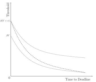
Figure 6: Comparing a Cost of Not Completing a Task With a Reward For Completing
Time to Deadline β(V +v)
βV
T
h
re
sh
o
ld
0
never face the cost of not completing the task before the deadline. Hence, the threshold approaches the baseline case in which no such penalty exists. Therefore, while imposing a penalty conditional upon not completing the task does impose some form of commitment, we would expect it to be weaker than the ability to convert an equivalent fixed payment to a reward which is conditional upon task completion.
4.3
Imposing a Penalty Per Time Period That the Task is not
Completed.
In the experiments of Ariely and Wertenbroch (2002) and in much of the theoretical literature (e.g., O’Donahue and Rabin (1999b)), rather than imposing a strict deadline beyond which the task cannot be completed, a weaker deadline is imposed. In particular, if the task has not been completed by a certain time period, say t∗, a per unit of time penalty is imposed.
Therefore, if the task is completed at time t > t∗, the reward is only V −(t−t∗)µ, where
µ >0 is the per period penalty. Comparing such a scheme with the strict deadlines that have been our focus thus far, a penalty for late completion provides only weaker incentives for early task completion, but it also does not destroy the option value of waiting. Therefore, in some circumstances it may be a useful commitment device for sophisticated decision makers. The appropriate question is then, what time t∗, after which a penalty for late completion
kicks in, would a decision maker set?
Figure 7 provides this answer for two cases. In each case the value for completing the task is ¯V = 1 and the penalty is 0.01 per unit of time.5 For simplicity, we also assumed that
the initial cost, x(0), of task completion is known with certainty. The result is similar to the case of a strict deadline: if β is sufficiently high, then the sophisticated decision maker prefers to choose a deadline sufficiently early so as to ensure immediate task completion. On the other hand, for β small, by setting an immediate deadline, the decision maker cannot compel her future self to complete the task immediately. In this circumstance, she prefers the latest possible deadline.
4.4
Allowing the Decision Maker to Self-Impose a Deadline
at
Any
Time.
A fourth approach is as follows. Suppose that the agent can impose a deadline on her future selves at any timet. That is, at any timet, once she realises x(t) she can impose a deadline strictly more binding than the current deadline. While this may seem like it complicates the
5
Figure 7: Numerical Results: Imposing a Penalty Per Time Period That the Task is not Completed
0 0.5 1 1.5 2 2.5 3 3.5 4 4.5 5 0.24
0.26 0.28 0.3 0.32 0.34 0.36
time at which penalty kicks in
Ex Ante Utility
Total Time: 5yrs; b = 0.8; r = 0.05; s = 0.2; x(0) = 0.5
0 0.5 1 1.5 2 2.5 3 3.5 4 4.5 5
0 0.005 0.01 0.015 0.02 0.025
time at which penalty kicks in
Ex Ante Utility
Total Time: 5yrs; b = 0.4; r = 0.05; s = 0.2; x(0) = 0.5
model a great deal, we argue that it simply reduces the model, for β not too small, to the case in which the agent has full commitment.
Let ¯xs(t) be the cutoff of a sophisticated hyperbolic agent at timet and let ¯xe(t) be the
cutoff of an exponential agent at time t. We know that ¯xs(t)<x¯e(t). Suppose now the cost
at timet,x(t)∈(¯xs(t),x¯e(t)). In this case , a sophisticated hyperbolic agent does not want
to complete the task but, importantly, she would prefer that her future self, at time t+ǫ, does complete the task.6 Therefore, she will set a deadline such that, with high probability,
x(t+ǫ) < x¯s(t+ǫ) < x¯e(t+ǫ). Indeed, since x follows a geometric Brownian motion as
the length of the time interval, ǫ, shrinks so does the variance (which is proportional to
σdt); therefore, as ǫ→0, an immediate deadline means that the new threshold is ¯xs=βV¯.
Provided thatβ is not too small, this will imply that ¯xs =βV <¯ x¯e(t).
This shows that a sophisticated hyperbolic agent who can impose deadlines at any mo-ment on her future selves will in fact do so, for every path of x which enters in the region of completion, provided that her self-control problems are not too severe. Therefore, with respect to task completion, such agents will behave (in a formal sense) identically to expo-nential agents.
5
Self-Imposed Deadlines in Other Models
Our analysis above suggests that self-imposed deadlines in the classic quasi-hyperbolic dis-counting framework are a relatively rare event. We now briefly discuss a few other models and
6
This follows because the continuation value,wc
their predictions regarding whether or not such decision makers would self-impose deadlines.
5.1
Temptation & Self-Control.
Miao (2008) adopts the temptation and self-control model of Gul and Pesendorfer (2001, 2004) to study the optimal exercise of various options in a discrete time, infinite horizon setting. When the cost of exercising the option is immediate, while the benefit is delayed, Miao shows that agents are tempted to delay, and therefore procrastinate. One can easily go beyond his analysis and ask whether the agent would like to bind herself by setting a deadline. In Appendix A, we consider the finite time version of Miao’s model and prove in Proposition 7 that the value function is increasing in the time to complete the task. Therefore, an agent with Gul-Pesendforfer preferences will not self-impose deadlines.
5.2
Optimal Expectations.
Brunnermeier, Papakonstantinou, and Parker (2007) propose a model of optimal expecta-tions in which decision makers will both procrastinate and self-impose binding deadlines. In their model, decision makers consistently under-estimate the amount of work required to complete a particular task, which leads to lower than optimal initial effort. However, the fact that the decision maker underestimates the required effort leads to an anticipatory utility effect: current felicity is boosted because he anticipates less work in the future. Thus these over-optimistic beliefs cause low initial effort, give an anticipatory boost to utility, but lead to extra future effort. The authors show that the ex ante utility benefits to over-optimism outweighs the ex post cost of poor planning; therefore, procrastination is, in some sense, optimal. Brunnermeier, Papakonstantinou, and Parker (2007) then show that agents will self-impose deadlines, which are less stringent than would be imposed by an outsider. It is this feature of their model which they claim is supported by the experimental evidence of Ariely and Wertenbroch (2002).
5.3
Misperceptions.
the task. Recall (1):
dx=σx·dz
where we assumed that the cost of completing the task follows a geometric Brownian motion, without drift. Two seemingly plausible misperceptions could be the following. First, it may be that the actual stochastic process for cost contains a drift term so that (1) becomes:
dx=αxdt+σx·dz
where α > 0 implies that the cost of completing the task is increasing over time. Under this altered model, we assume that β = 1 and redefine the “current” and “future” selves as follows: the current self is aware of the drift term, while the future self believes that α = 0. All other aspects of our model remain unchanged. Now, in this model, when a decision maker is faced with a high cost of task completion, she thinks that it was due to a high realization ofdz, rather than due to positive drift. Therefore, she may not complete the task now because she (incorrectly) expects the cost to be lower in the future.
Now consider the decision maker at time 0 who is aware of her problems with misper-ception. Because α >0, as time passes, it becomes increasingly less likely that the decision maker will complete the task. Therefore, the option value of having extra time is much less valuable, while the commitment benefit of a deadline remains, making it much more likely that the time 0 self will set a deadline.
As an alternative to the drift term, one could assume instead that the stochastic process for costs actually follows a jump-diffusion. That is, there is some Poisson arrival rate at which the cost of completing the task “jumps” by a discrete, positive amount. In this model, with a similar reinterpretation of the current and future selves, the presence of misperceived jumps also mitigates the option value of having extra time to complete the task, making self-imposed deadlines much more likely.
6
Conclusions
makers will complete a task. While an exponential discounter has a threshold at every time
t, and will complete the task if the cost of doing so is less than the threshold, a na¨ıf will never complete the task strictly before the deadline. Therefore, such decision makers suffer from a very extreme form of procrastination.
In contrast, our model shows that sophisticates will sometimes self-impose a deadline. The reason for this is because, ex ante there is a discontinuous benefit to immediately completing the task. On the other hand, if the task is not completed immediately, then our results show that the sophisticated decision maker behaves like an exponential decision maker, but with a lower value of task completion. Consequently, if the task is not immediately completed, the sophisticated decision maker (just like an exponential discounter) prefers to have as much time as possible to complete the task. Thus there is a kind of bang-bang property of self-imposed deadlines. Either the sophisticated decision maker prefers an immediate deadline or no deadline at all. Somewhat surprisingly, the decision maker will never set an intermediate deadline.
While our model has focused on a single task, it can also be extended to multiple tasks. However, care must be taken on this front for it seems that without further alterations, this extended model would predict identical threshold for all tasks. That is, as soon as the decision maker completes one task, she will also complete the rest. Instead, it seems likely that fatigue might set in. To capture this, one could include a discrete (perhaps deterministic) increase in cost upon the completion of a single task. Therefore, once a decision maker completes one task, her cost will increase, forcing her to “relax” and wait for a lower cost to arise in the future. This could be why Ariely and Wertenbroch (2002) found that evenly spaced deadlines were the most effective.
With somewhat greater difficulty, our model could also be extended to continuous tasks (i.e., tasks that require the exertion of effort for some, possibly random, amount of time). This adds an additional layer of complication since it introduces another state variable — the amount of exertion required to complete the task — turning the decision problem into a control problem. However, such an extended model could easily be parameterized to reconcile the cycles found in Study 1 of Burger, Charness, and Lynham (2009). In particular, instead of the geometric Browning motion used to model the evolution of opportunity costs, one could work with a mean reverting process with cycles.
References
Ariely, D., and K. Wertenbroch (2002): “Procrastination, Deadlines, and
Brunnermeier, M., F. Papakonstantinou, and J. Parker (2007): “An Economic Model of the Planning Fallacy,” Working Paper.
Burger, N., G. Charness, and J. Lynham (2009): “Three Field Experiments on
Pro-crastination and Willpower,” Working Paper.
Carr, P., R. Jarrow, and R. Myneni(1992): “Alternative Characterizations of
Amer-ican Put Options,”Mathematical Finance, 2, 78–106.
Cox, J. S., S. Ross, and M. Rubinstein (1979): “Option Pricing: A Simplified
Ap-proach,”Journal of Financial Economics, 7, 229–263.
Dixit, A., and R. Pindyck (1994): Investment Under Uncertainty. Princeton University
Press, Princeton, N.J.
Gul, F., and W. Pesendorfer (2001): “Temptation and Self-Control,” Econometrica,
69, 1403–1436.
(2004): “Self-Control and the Theory of Consumption,”Econometrica, 72, 119–158.
Harris, C., and D. Laibson (2004): “Instantaneous Gratification,” Working Paper.
Hsiaw, A. (2008): “Goal-Setting, Social Comparison, and Self-Control,” Working Paper.
Hull, J. C. (2005): Options, Futures & Other Derivatives. Prentice Hall, Upper Saddle
River, N.J., 6th edn.
Laibson, D. (1994): “Essays in Hyperbolic Discounting,” Ph.D. thesis, Massachusetts
In-stitute of Technology.
(1997): “Golden Eggs and Hyperbolic Discounting,”Quarterly Journal of Econom-cis, 113, 443–477.
Miao, J.(2008): “Option Exercise With Temptation,” Economic Theory, 34, 473–501.
O’Donahue, T., and M. Rabin (1999a): “Doing It Now or Later,” American Economic
Review, 89(1), 103–124.
(1999b): “Incentives for Procrastinators,” Quarterly Journal of Economcis, 114, 769–816.
Peskir, G., and A. Shiryaev (2006): Optimal Stopping and Free Boundary Problems.
Phelps, E. S., and R. Pollak (1968): “On Second-Best National Saving and Game-Equilibrium Growth,” Review of Economic Studies, 35, 185–199.
S´aez-Mart´ı, M., and A. Sj¨ogren (2008): “Deadlines and Distractions,” Journal of
Economic Theory, 143, 153–176.
Trope, Y., and A. Fishbach (2000): “Counteractive Self-Control in Overcoming
A
Temptation and Self-Control
In this appendix we discuss the work of Miao (2008) and formally show that the a decision maker with Gul-Pesendorfer preferences will never choose to self-impose a binding deadline. Recall that if the agent faces a choice set Bt when there are t periods remaining and Wt is
the agent’s intertemporal utility, then self-control preferences `a la Gul-Pesendorfer are given by:
Wt(Bt) = max ct∈Bt
{u(ct) +δE[Wt−1(Bt−1)] +vt(ct)} −max ct∈Bt
vt(ct)
where Bt ={0,1} provided that for all periods n > t, cn = 0; that is, the agent can either
complete the task or wait, and once she has completed the task, the decision problem ends and the agent receives the appropriate payoffs. Let c∗
t denote the optimal choice, then an
agent with such preferences suffers a utility loss due to temptation ofvt(c∗t)−maxc∈Btvt(c).
It is this utility loss due to temptation which causes procrastination; in particular, the temptation to delay exerting costly effort. Miao (2008) then specialises to stopping time problems and considers three cases: immediate costs, immediate rewards and both immediate costs and rewards, and the reader is referred to his paper (specifically, Section 3.1) for more details. The case that is relevant for us is that of immediate costs. While Miao considers an infinite horizon problem, his model is easily adapted to a finite horizon setting. We also adapt his model to make the reward from task completion known, but the cost of completion stochastic. In no way does this change the results. Denote the value function when there are t periods remaining as:
Wt(x) = max{δV −(1 +γ)x, δ
Z
Wt−1(x′)dF(x′)} −γmax{0,−x}
= max{δV −(1 +γ)x, δ
Z
Wt−1(x′)dF(x′)}
where,V is the known and deterministic benefit from completing the task, xis the stochastic realisation of the cost of task completion, and F(·) is the distribution function from which the cost of task completion, x is drawn. The second equality follows from the fact that
x ≥ 0; therefore, max{0,−x} = 0. Of course, notice that W0(x) ≡ 0. Since the benefit
of completing the task is delayed by one period, we must discount the reward - hence the appearance of the termδV; on the other hand, the cost of task completion cost, denoted by
x, is stochastic. Finally,γxis the cost of exercising self-control and immediately completing the task.
We claim the following:
Proposition 7. Wt+1(x)≥Wt(x) for all t and x.
for x < δV
1+γ and zero otherwise, the result is true for t= 0. Next suppose that the result is
true for all t = 0,1, . . . , nWe now show that Wn+1(x)≥Wn(x). Observe that:
Wn+1(x) = max{δV −(1 +γ)x, δ
R
Wn(x′)dF(x′)}
≥ max{δV −(1 +γ)x, δR
Wn−1(x′)dF(x′)}
= Wn(x)
where the inequality follows from our induction hypothesis that Wn(x) ≥ Wn−1(x). Hence
the result follows.
Of course, while Proposition7shows that a decision maker with such preferences prefers the latest possible deadline, that is not to say that she will not procrastinate. In particular, one can easily show that the threshold cost of task completion is decreasing in γ, which measures the cost of self-control.
B
The Finite
λ
Case
Our discussion so far has always concerned itself with the limiting case of λ→ ∞. However, one may also be interested in the finiteλ case where the present self can expect to exercise control for a measurable time interval. In particular, this issue of the agent’s willingness to self-impose a binding deadline arises again. Recall that forλ=∞, so that the sophisticated agent knows that he will exercise control only for an infinitesimal length of time, self-imposed deadlines are a relatively rare occurrence.
We claim that our model is continuous in λ in the following sense. Rewrite (12):
Ws(x, t) = max{U(λ)−x , e−ρdtE
e−λdtWs(x+dx, t+dt)
+(1−e−λdt)βwc(x+dx, t+dt)
The reason for this continuity in λ is as follows. Despite being sophisticated, and therefore knowing that his future self will not complete the task for high enough realisations of the cost, the decision maker is tempted to delay because with probability 1−e−λdt, the agent