Munich Personal RePEc Archive
The Almost Ideal and Translog Demand
Systems
Holt, Matthew T. and Goodwin, Barry K.
Purdue University, North Carolina State University
14 March 2009
The Almost Ideal and Translog Demand
Systems
Matthew T. Holt
∗Department of Agricultural Economics Purdue University
Barry K. Goodwin
†Department of Agricultural and Resource Economics North Carolina State University
This Draft: March 13, 2009
Abstract
This chapter reviews the specification and application of the Deaton and Muellbauer (1980) Almost Ideal Demand System (AIDS) and the Christensen, Jorgenson, and Lau (1975) tranlog (TL) demand system. In so doing we examine various refinements to these models, including ways of incorporating demographic effects, methods by which curvature conditions can be imposed, and issues associated with incorporating structural change and seasonal effects. We also review methods for adjusting for autocorrelation in the model’s residuals. A set of empirical examples for the AIDS and a the log TL version of the translog based on historical meat price and consumption data for the United States are also presented.
Keywords: Almost ideal demand system, Autocorrelation, Curvature, Meat Demand, Translog
JEL Classification Codes: D12; C32; Q11
∗Department of Agricultural Economics, Purdue University, 403 W. State Street, West Lafayette, IN
47907–2056, USA. Telephone: 765-494-7709. Fax: 765-494-9176. E-mail: mholt@purdue.edu.
†Department of Agricultural and Resource Economics and Department of Economics, North Carolina
1
Introduction
The now classic paper by Deaton and Muellbauer (1980) established a standard for applied
demand analysis in the “Almost Ideal Demand System” or AIDS model. The fundamental
demand model established by this paper has realized very widespread application in
con-sumption analysis. The Social Science Citation Index shows that this paper has been cited
822 times (as of January 23, 2009). A closely related alternative—the “Transcendental
Log-arithmic” or “translog” demand system has also realized widespread application in demand
analysis. The classic paper by Christensen, Jorgenson, and Lau (1975) that introduced the
translog consumer demand system has been cited 361 times according to the Social Science
Citation Index. In both cases, the tabulated citations clearly understate the impact of these
two pioneering demand models. As is often the case, such classics become standard, accepted
practice and thus many practitioners fail to cite the papers that originated the methods and
instead depend upon widespread recognition of the models and methods.
As we discuss in this chapter, both demand system models are often motivated within the
context of “flexible functional forms” that provide certain advantages in terms of minimizing
specification biases in representing demand systems of unknown forms. In addition to its
flexibility properties as a first-order approximation to any demand system, the AIDS model
also possesses certain nonlinear aggregation properties that make it “almost ideal” for applied
work.
In this chapter, we provide a broad overview of the AIDS and translog demand systems.
We discuss practical issues relating to their utilization in applied demand analysis. We also
outline a number of closely related issues that typically arise in the application of these
mod-els. These issues include incorporation of seasonality and structural change, representation
of autocorrelation within a singular system of equations of the sort inherent in the AIDS and
translog models, and inequality restrictions that are implied by concavity of the underlying
utility function. We illustrate these practical issues associated with applying each model
this paper is on the practical and applied issues associated with the use of these demand
models and thus we refer the reader to the original sources as well as to a very large collection
of other applied papers for greater detail on many of the issues that we address.
2
Specification of the Almost Ideal Demand System
The basic AIDS model is developed from a particular cost (expenditure) function taken from
the general class of “price-independent, generalized logarithmic” or PIGLOG cost functions.
In the case of the AIDS the cost function is of the form
lnC(p, U) = (1−U) ln(a(p)) +Uln(b(p)) (1)
where p is a nx1 vector of unit prices, U denotes the utility index, a(p) is a translog price
index given by
lna(p) =α0 +
X k
αkln(pk) +
1 2
X k
X j
γ∗
kjlnpklnpj, (2)
and
lnb(p) = lna(p) +β0
Y k
pβk
k . (3)
As well, k, j = 1, . . . , n. Note that the utility index can be scaled to correspond to cases of
subsistence (U = 0) and bliss (U = 1), in which case, a(P) and b(P) can be interpreted as
representing the cost of subsistence and bliss, respectively.
Application of Shephard’s Lemma through differentiation of the logarithmic cost function
with respect to a logarithmic price yields budget (expenditure) share equations for each good
in the utility function. We can “uncompensate” the share equations to remove utility by
noting that total expenditure, (y), for a utility-maximizing consumer will equal the value of
the cost function. We may therefore invert the cost function and solve for U, the indirect
utility function υ(p, y). Finally, υ(p, y) may be used to substitute for U in each share
Doing so yields share equations of the form:
wi =αi+ X
j
γijlnpj+βi(ln(y)−ln(P)) (4)
where wi = piyqi, i= 1, . . . , n, and P is a price index defined by
lnP =α0+
X k
αkln(pk) +
1 2 X k X j
γkjlnpklnpj, (5)
and where γij =
1
2(γij∗ +γji∗).
Linear homogeneity of the cost function, symmetry of the second–order derivatives, and
adding–up across the share equations implies the following set of (equality) restrictions:
n X
i=1
αi = 1, n X
i=1 γij =
n X
j=1
γij = 0, n X
i=1
βi = 0, γij =γji. (6)
As required for a locally flexible functional form, there aren(n−1)/2 free parameters in the
Slutsky matrix for the AIDS model.
Using the familiar result that uncompensated (Marshallian) price elasticities in any
de-mand system are given by −δij + ∂
lnwi
∂lnpj, where δij is the Kronecker delta term, the price
elasticities in the AIDS model are given by
ηij =−δij +
γij −βi(αj+ P
kγjklnpk)
wi
. (7)
Note here also that in practice the term given by (αj +Pkγjklnpk) may sometimes be
replaced by the equivalent (wj−βjln(y/P)) in elasticity expressions. Expenditure (income)
elasticities are given by:
ηiy =
βi
wi
+ 1. (8)
Slutsky equation. In elasticity form this equation yields:
ηc
ij =ηij +wjηiy, (9)
whereηc
ij denotes the compensated price elasticity forith good with respect to the jth price.
Deaton and Muellbauer (1980) proposed replacing the nonlinear AIDS price index in 5
with an appropriately specified price index that can be defined outside of the AIDS system,
thus leaving a purely linear system of share equations. Specifically, they suggest Stone’s
share-weighted geometric mean price index as an obvious candidate:
lnP∗ =
N X
i=1
wiln(pi). (10)
This version became known as the “Linear–Approximate” AIDS model, or LA–AIDS. This
suggestion by Deaton and Muellbauer (1980) led to much consternation and debate over,
among other things, the appropriate specification of the LA–AIDS elasticities and the overall
properties of the LA–AIDS model. For example, Moschini (1995) shows that the Stone
in-dex in (10) is not invariant to units of measurement, although normalizing all prices by their
respective sample means does circumvent this problem. As well, Eales and Unnevehr (1988)
note that when Stone’s index is used that budget shares also appear on the right–hand side
of the equations. Likewise, Buse (1998) comments on the “errors in variables” problems
in-troduced by using the Stone index in lieu of the true translog index. Finally, Lafrance (2004)
examines the integrability properties of the LA–AIDS, finding that very restrictive forms are
implied for the underlying expenditure function when symmetry conditions are imposed. In
any event, all issues pertaining to the specification, estimation, and interpretation of the
LA–AIDS are rendered moot if instead the translog price indexa(p) in (5) is simply used in
estimation. Even so, it is often useful to estimate the LA–AIDS for purposes of obtaining
starting values in estimation of the AIDS model with the nonlinear price index (Browning
3
Specification of the Translog Demand System
A closely related demand model is found in the “Transcendental Logarithmic” or “translog”
(TL) demand system of Christensen, Jorgenson, and Lau (1975). The translog consumer
de-mand system is usually derived by applying Roy’s Identity to a quadratic, logarithmic
specifi-cation of an indirect utility function written in terms of expenditure-normalized prices.
Nor-malizing each price by dividing by total expenditures imposes homogeneity. The quadratic,
logarithmic indirect utility function is given by:
ln Ψ(p, y) =α0+
X k
αkln(pk/y) +
1 2 X k X j
γkjln(pk/y) ln(pj/y), (11)
k, j = 1, . . . , n. It is relevant to note the similarity of the translog specification to the price
index inherent in the AIDS model as specified in (2). Applying the logarithmic version of
Roy’s identity to the indirect utility function in (11) yields share equations of the form:
wi =
αi+Pkγikln(pk/y) P
m(αm+ P
kγmkln(pk/y)
, (12)
where again i = 1, . . . , n. Note that the denominator of the share equation in (12) is the
sum of the numerators across all shares. This is often written in an equivalent form as:
wi =
αi+Pkγikln(pk/y)
αM + P
kγM kln(pk/y)
, (13)
where αM = PM
i=1αi and γM k =
PM
i=1γik and where, of course, M = n. Note also that
the parameters are given in ratio form and thus are only identified to scale. A common
normalization to allow identification is to setαM = P
iαi =−1.
Homogeneity is necessarily guaranteed in the standard translog model in light of the use
of expenditure-normalized prices. Symmetry requires γij =γji. In the case of the TL there
are n(n+ 1)/2 free parameters in the Slutsky matrix, thereby implying that the translog has
form.
Uncompensated price elasticities in the translog are given by:
ηij =−δij +
γij/wi−Pjγij
−1 +P
kγM kln(pk/y)
. (14)
Expenditure elasticities are given by:
ηiy= 1 +
−P
jγij/wi+ P
i P
jγij
−1 +P
kγM kln(pk/y)
. (15)
As in the case of the AIDS, compensated (Hicksian) price elasticities may be determined by
using (9).
There is a variant of the translog model that is often used in practice, the log tranlog
(log TL) or aggregatable tranlog. See, Pollak and Wales (1992). The basic log TL may be
derived from the TL by simply imposing the additional restriction that P
kγM k = 0. Of
course doing so reduces the number of free parameters in the model by one so that now
there are n(n+ 1)/2−1 free parameters in the Slutsky matrix. In any event even the log
LT has more free parameters then are required for the system to satisfy the properties of a
second–order (locally) flexible functional form.
Finally, any discussion of the AIDS and translog models would be remiss without explicit
mention of the fact that the two models are of a very similar analytical structure. This
similarity has led to efforts to directly compare the two closely–related specifications. A
notable example exists in the work of Lewbel (1989), who developed a demand model that
nests both the AIDS and the translog demand systems. Lewbel (1989) develops a more
general model that nests both the AIDS and the translog systems as special cases defined
by parametric restrictions which can, in turn, be used to pursue nested specification testing
of each alternative. Lewbel (1989) applied this model to aggregated U.S. expenditure data
and found that the explanatory power and statistical fit of the alternative models were very
conclusions reached in our own empirical example presented below.
4
Issues in Applying the AIDS and Translog Models
A variety of issues and concerns may apply to any specific application of the AIDS and
translog models. These issues may arise as a result of characteristics of the data. For
example, issues relating to seasonality and structural change may arise in applications using
data collected over time. Likewise, data aggregated across households may raise questions
regarding the aggregation properties of a particular demand model. Methods for imposing
the curvature constraints inherent in the aforementioned conditions required for concavity
also raise important modeling questions. The treatment of autocorrelation in a singular
system of share equations may be important in applications to time-series data. Both the
AIDS and translog demand systems are nonlinear in the parameters, though practice has
shown the AIDS model to be relatively straightforward to estimate while the degree of
nonlinearity inherent in the translog model may result in additional estimation challenges.
4.1
Aggregation Properties
Empirical applications of demand system models typically proceed according to one of two
approaches. The first uses data collected from individuals or, more commonly, from
house-holds. Such paths to analysis typically assume a common underlying structure for tastes
and preferences and commonly apply various demographic shifters or adjustments to reflect
differences across individuals. A second approach to empirical analysis involves the use of
more aggregate data collected over groups of individuals or households and most often taken
across multiple time periods. In this case, one must consider aggregation properties that
reflect the extent to which the demand estimates accurately represent the underlying
pref-erence structure reflecting the optimizing choices of individuals making up the aggregate.
consumer defined at average values of prices and income. In their text, Deaton and
Muell-bauer (1980) note that “. . . in general, it is neither necessary, nor necessarily desirable, that
macroeconomic relations should replicate their microfoundations so that exact aggregation
is possible.”
It is common to assume that perfectly integrated goods markets result in a common price
for a good of a certain defined (homogeneous) quality. However, when aggregating across
households, differences in income will clearly exist and thus conditions for exact aggregation
should be considered. One of the AIDS model’s “almost ideal” properties relates to its
aggregation properties. In particular, the AIDS model satisfies exact nonlinear aggregation
because the cost function upon which it is based is of a specific functional form for underlying
preferences known as a “price independent generalized logarithmic” (or PIGLOG) form. This
allows one to work with a representative measure of household expenditure, defined as y0.
Deaton and Muellbauer (1980) show that, in the AIDS model case,y0is given byy0 =κ0y¯,
where κ0 =H/Z where H is the number of households or individuals making up the
aggre-gate and Z is Theil’s entropy measure of dispersion of income across individual units. Note
further here that, if the number of households and the distribution of income is constant
across individual aggregate measures (i.e., aggregated time-series observations), the AIDS
model satisfies exact nonlinear aggregation without further adjustment. If either the number
of households or the distribution of income varies across the sample of aggregated data, a
straightforward adjustment to the average level of household income can be applied to
main-tain desirable aggregation properties. Some applications of the AIDS model to aggregate
data apply Theil’s entropy index correction to average income levels to ensure valid
aggre-gation properties. One example can be found in Eales and Unnevehr (1988), who adjusted
4.2
Flexibility and Model Extensions
The AIDS model is derived from an expenditure function that can be interpreted as a
second-order approximation to an arbitrary unknown function. As Deaton and Muellbauer (1980)
note, the AIDS demand system can thus be interpreted as a first-order approximation to
any demand system. Having noted these desirable flexibility properties, other authors have
considered amendments to the basic AIDS structure in an effort to improve or enhance its
flexibility properties.
Banks, Blundell, and Lewbel (1997) introduced a quadratic version of the standard AIDS
model that adds a quadratic logarithmic income term and nests the standard AIDS model
specification. The resulting QUAIDS model is given by share equations of the form
wi =αi+ X
j
γijlnpj +βiln(y/P) +
λi Q
ip βi
i
(ln(y/P))2
(16)
where P is the AIDS price index.
Other approaches to adding flexibility to the standard AIDS model have been proposed
in other research. Chalfant (1987) augmented the AIDS expenditure function by replacing
the translog cost function terms with Fourier series expansion terms. This specification also
nests a standard AIDS model and thus permits straightforward specification testing. As
Gallant (1981) has shown, the Fourier flexible form may offer more global flexibility than is
the case for the translog demand system.
Another extension to the standard AIDS model was proposed by Eales and Unnevehr
(1994), who considered applications where the quantities tended to be fixed in the short-run
and thus where prices adjusted to clear the market. Eales and Unnevehr (1994) discussed
specific applications where exogenous quantities may be more reasonable than exogenous
prices. Specific examples include short-run demand for perishable commodities, commodities
which are subject to long production lags and thus are essentially in fixed supply in the
exogenously fix quantities.
The inverse AIDS model (IAIDS) is entirely analogous to the standard AIDS model. The
model is defined using a logarithmic distance function that is specified in a manner that is
entirely analogous to the expenditure function. Differentiation of the logarithmic distance
function yields share equations that are expressed as a function of quantities and utility.
Substitution of the inverted distance function uncompensates the functions and yields a
system of inverse demand share equations of the form:
wi =αi+ X
j
γijlnqj +βiln(Q) (17)
where Qis a quantity index defined by
lnQ=α0+
X k
αkln(qk) +
1 2 X k X j
γkjlnqklnqj. (18)
As illustrated by Christensen and Manser (1977), an inverse counterpart to the translog
model, the ITL, is also available. Specifically, the direct utility function as being of a translog
form. Specifically, the utility function may be specified as:
−lnU =α0+
X k
αkln(qk) +
1 2 X k X j
γkjlnqklnqj, (19)
where γij = γji. By maximizing (19) subject to the budget constraint p′q = y, and then
applying the so–called Hotelling–Wold identity (Hotelling 1935), a system of inverse demand
equations of the general form
wi =
αi+Pkγikln(qk)
αM + P
kγM kln(qk)
, (20)
obtains. As with the IAIDS, the ITL in (20) is in every respect analogous to the direct TL
4.3
Seasonality, Demographics, and Structural Change
In applications of the AIDS and translog demand systems to time-series data, one may need
to be concerned with the potential for exogenous shifts in the underlying structure of the
economic relationships represented by the model. The tastes and preferences underlying
observed demand relationships may be subject to temporary or permanent structural shifts.
This may reflect a change in preferences or the arrival of new information that is
embed-ded in prices. Alternatively, if one is working with quarterly data, seasonal patterns may
characterize consumption. It is important to recognize that any such adjustment necessarily
implies analogous changes in the underlying utility maximization behavior of agents.
It is common practice to include exogenous intercept shifters in the basic AIDS and
translog share equations to capture the effects of structural change, seasonality, or other
exogenous shifters. In doing so, one must be careful to pay attention to the adding up
conditions represented above in order to ensure that the addition of such shifters does not
violate adding up across equations. A common approach to representing a linear shift in
expenditure shares that does not reflect changes in prices or income is to add a simple
linear trend to the share equations, which is analogous to allowing the intercept term of
each share equation to trend such that αit =αi0+αitt where t = 1, . . . , T. In such a case,
one would recover the trend of the last omitted equation from the adding up condition that
requires P
kαkt = 0. This same general intuition carries over to more complex shifters
that allow the intercept to shift according to the quarter of the year of the observation or
even other shifters such as demographic terms. We should note that an entire literature
has developed to address the incorporation of demographic translation and scaling terms in
empirical demand models. For our purposes here, it suffices to note that attention to adding
up must accompany any amendments to the underlying AIDS or translog share equations
intended to allow the structure to vary outside of price and income changes. In the case of
adjustments for seasonality, one may add a series of indicator variables intended to capture
amended to incorporate seasonality by expressing the intercept terms asαis =αi0+P 3
s=1δsS
where S is one if the quarter is dated s=S and is zero otherwise.
4.4
Imposing Curvature
One issue that arises frequently in estimation of demand systems is the imposition of
cur-vature (negativity) conditions (Barten and Geyskens 1975). Basic microtheoretic results
indicate that in order for integrability of the system to hold that the n×n Slutsky matrix
will be symmetric and that it will be, at most, of rankn−1. As well, quasi–concavity of the
utility function implies that the Slutsky matrix will be negative semi–definite. One
immedi-ate implication is, of course, that Hicksian (compensimmedi-ated) demands will be non–increasing
in own price. In any event, whether or not curvature conditions are satisfied at all or even
for any points in the sample data is a relevant issue, and one that should be examined in
any empirical investigation.
As illustrated by Moschini (1998) and Ryan and Wales (1998), the Slutsky matrix for the
AIDS and the TL models assume rather simple forms when evaluated at the points p∗ = ι
andy∗ = 1, whereιis an×1 unit vector. Specifically, theijth element of the Slutsky matrix
for the AIDS model is given by
Sij =γij −(αi−βiα0)δij −(αj−βjα0)(αi−βiα0) +βiβjα0, (21)
where δij is the Kronecker delta term. Moreover, if α0 is restricted to zero–a normalization
that is often used in empirical applications of the AIDS model–theijthelement of the Slutsky
matrix in (21) reduces to
Sij =γij −αiδij −αjαi. (22)
p∗ =ι and y∗ = 1, is given by
Sij =−γij +αiαj+αiδij −αi X
k
γkj −αj X
k
γik−αiαj X
k X
j
γkj. (23)
Of course for the log TL model the ijth element of the Slutsky equation simply reduces to
Sij =−γij+αiαj+αiδij −αi X
k
γkj−αj X
k
γik. (24)
The expressions in (21)–(24) can be used to construct the relevantn×nSlutsky matrix. From
here it is then possible to calculate the eigenvalues of the Slutsky matrix and to determine
whether or not the lead eigenvalue is zero at the point of approximation.
Aside from checking to determine whether or not the curvature conditions are satisfied,
it may be desirable to impose the non–negativity conditions during estimation. There are
various ways of accomplishing this task, including both classical and Bayesian approaches.
For example, Gallant and Golub (1984) propose imposition of inequality constraints directly
on eigenvalues in the context of a maximum likelihood estimation routine. Alternatively,
Chalfant, Gray, and White (1991) build off of a Bayesian approach introduced originally by
Geweke (1993) that uses importance sampling in conjunction with Monte Carlo simulation to
impose curvature in an AIDS demand system. An essentially identical approach was adopted
by Terrell (1996) for purposes of imposing curvature conditions in a TL cost function.
More recently, several authors have investigated ways of reparameterizing the Slutsky
matrix so that curvature may be directly imposed at a point during estimation. All of these
procedures essentially build on results presented initially by Diewert and Wales (1988a,
1988b) in the context of imposing curvature globally in their normalized quadratic (NQ)
demand system. For example, Moschini (1998) and Ryan and Wales (1998) show how the
Diewert and Wales approach may be adopted to impose curvature at a point in the AIDS
model.
˜
A is a n ×n lower triangular matrix. Of course, due to the fact that Hicksian demands
are homogeneous of degree zero in prices, all relevant price vectors lie in the null space of
Slutsky matrix, S. If, for example, prices are normalized to have a unit mean, then it would
necessarily be true that Sι = 0 as well. The implication is that the Slutsky matrix can be
written in terms of its Cholesky decomposition as
−S =AA′ = A˜A˜′ ˜a
˜
a′ −ι′˜a′
!
(25)
where
˜
A =haij i
, aij = 0 ∀j > i, i, j = 1, . . . , n−1,
and where the kth element of the (n−1)×1 vector ˜a is given by ˜a
k =Pn−
1
j akj. Now, let
(−A˜A˜′)
ij denote theijthelement of−A˜A˜′. Then (22), after solving forγij, may be expressed
alternatively as
γij = (−A˜A˜′)ij +αiδij −αjαi. (26)
Specifically, it is the coefficients in the (n−1)×(n−1) lower triangular matrix ˜A that are
estimated in lieu of the γij terms when curvature is imposed at the p∗ =ι and y∗ = 1 point.
As discussed originally by Diewert and Wales (1988b), if it is necessary to impose
curva-ture by using the Cholesky decomposition, then the leading non–zero eigenvalue in −AA′,
while negative, will often be near zero. Diewert and Wales (1988b) show that the rank of
−A˜A˜′ can be restricted to some K < (n−1) by setting a
ij = 0 for all i > K. In turn
re-stricting−A˜A˜′ in this manner will, via (25), restrict the rank of S toK < n−1, resulting in
what Diewert and Wales refer to as a semiflexible form when combined with their normalized
quadratic demand system. An interesting feature of this approach is that once curvature is
imposed the rank of the Slutsky matrix can be successively reduced until noticeable harm is
done to model fit, perhaps as measured by the Akaike information criterion (AIC) or some
other model selection criterion. In his 1998 study Moschini used these results in conjunction
Finally, Moschini (1999) show shtat similar procedures may be applied to reparmaterized
versions of the TL and log TL models, again for purposes of imposing curvature at a point.
Furthermore, Ryan and Wales (1998) illustrate that in many instances curvature conditions
may be forced to hold at all sample points if the sample point for which the violation is most
stringent is used as the point for data normalization, that is, the point for which prices and
expenditure are normalized to have unit values.
4.5
Stochastic Specification and Autocorrelation
An area of key interest in demand system estimation, at least when time series data are
em-ployed, is the inclusion of autocorrelation terms in stochastic share equation specifications.
Because share equations must necessarily satisfy adding–up properties at all data points,
it is not possible to specify autocorrelation terms without imposing additional restrictions
(Berndt and Savin 1975). Here we briefly review the unique requirements of autocorrelation
specifications in systems of singular share equations along with several popular
autocorrela-tion models used in practice.
To begin, we follow Barten (1969) who illustrates that, for system’s of equations subject
to adding–up conditions, that: (1) in estimation an equation must be deleted since the
resultant n ×n covariance matrix is not of full rank, and therefore an equation must be
omitted in estimation; and (2) that iterative Seemingly Unrelated Regression (SUR) yields
maximum likelihood estimates of the system’s parameters that are, moreover, invariant with
respect to the equation that is deleted. Specifically, let a superscripted napplied to a vector
(matrix) denote an operator that deletes the last row (row and column) of a vector (matrix).
In this case we might then represent then−1 equation system to be estimated as:
wn t =f
n(z
t, θ) +ent, t = 1, . . . , T, (27)
where wn
including prices and income, θ is a vector of unknown parameters to be estimated, anden t is
an (n−1)–vector of mean zero random error terms.
Now assume that the errors in (27), that is, the elements inen
t, are autocorrelated, as is
of-ten the case when time series data are employed. Moreover, assume that the autocorrelation
follows a first–order vector autoregressive process. That is,
en t =R
n
et−1+εnt, t = 2, . . . , T, (28)
where R is an (n−1)×(n−1) autocorrelation matrix and εn
t is a (n−1)×1 error vector
such that E(εn
t) = 0, E(εnt(εnt)′) = Ω, andE(εnt(εns)′) = 0 ∀t6=s. By substituting the vector
autoregressive error process in (28) into (27) the following quasi-differenced equation system
obtains:
wn t =f
n(z
t, θ) +R n
[wn t−1−f
n(z
t−1, θ)] +εnt, t= 2, . . . , T. (29)
As outlined by Moschini and Moro (1994) and Holt (1998) there are at least five ways to
parameterize the autocorrelation matrix Rn in (28), including the unrestricted specification outlined by Anderson and Blundell (1982) and the single–parameter specification suggested
by Berndt and Savin (1975). In the empirical application that follows we utilize the
pos-itive semi–definite parametrization for Rn advanced by Holt (1998), which is often found to provide reasonable flexibility (relative to the single–parameter case) and yet maintains
reasonable parsimony (relative to the unrestricted case). In short, the positive semi–definite
set–up applies the same same procedures to the autocorrelation matrix that Diewert and
Wales (1988a, 1988b) use to impose negativity on the Slutsky matrix of a demand system.
The positive semi–definite specification is defined as follows. Assume the n×n
Holt (1998) describes how, with the foregoing restriction, theR matrix may be specified as:
R= R˜ ˜r ˜
r′ −ι′˜r′
!
(30)
where
˜
R =T T′, T =hτ
ij i
, τij = 0 ∀j > i.
A typical element in the (n−1)×1 vector ˜r is rk = Pn−
1
j=1 R˜jk. Moreover, as specified in
(30) the (n−1)×(n−1) matrixT is a lower-triangular matrix; it is the elements in T that
are estimated directly by using Holt’s (1998) method.
Alternative methods for dealing with demand systems in the context of time series data
have been explored by Anderson and Blundell (1982), Ng (1995), Attfield (1997),
Kara-giannisa and Mergos (2002), and Lewbell and Ng (2005). The basic idea is that prices,
expenditure, and perhaps budget shares follow something akin to a unit root process,
im-plying that the data should be first differenced as a prelude to estimation. Moreover, if
the underlying demand system is linear in variables—as it is for the AIDS model when a
Stone (or other) price index is used to replace the nonlinear price index a(p) in (2)—then
it is also possible to examine cointegration properties in the context of a demand system.
Alternatively, Lewbell and Ng (2005) propose a variant of the translog model that can also
be used to estimate demand systems in the context of nonstationary data. Although holding
promise, one limitation of the time series approach to demand system estimation is that
shares are, by definition, bounded on the unit interval, a result that is in turn inconsistent
with unit root behavior and therefore with first differencing. See, for example, the discussion
in Davidson and Ter¨asvirta (2002). Future work may therefore focus on the possibility that
5
An Empirical Example
In this section we provide a stylized application of the AIDS and translog demand systems in
the context of time series data. Specifically, we illustrate the application of these models to
aggregate meat demand data in the United States. Indeed, there is a long tradition of using
various demand systems, including both the AIDS and the translog models, to investigate
the properties of U.S. meat consumption. See, for example, Christensen and Manser (1977),
Moschini and Mielke (1989), and Piggott and Marsh (2004), among others. It therefore is
reasonable to illustrate the properties of these demand systems in the context of aggregate
meat demand data in the United States.
5.1
Data
Quarterly data on consumption and retail prices for beef, pork, chicken, and turkey were
col-lected from various USDA sources for the 1960–2004 period. Data prior 1997 were obtained
from various sources described in some detail by Holt (2002). Data for pork and beef from
1997 through 2004 were obtained from the online version of the U.S. Department of
Agricul-ture (2006b) Red Meat Yearbook. Likewise, data for chicken and turkey were obtained from
the online version of the U.S. Department of Agriculture (2006a)Poultry Yearbook. Similar
to Piggott and Marsh (2004), we aggregate the chicken and turkey categories to obtain a
single “poultry” category. The retail price for poultry is derived by determining the share–
weighted averages for chicken and turkey prices where the shares are with respect to total
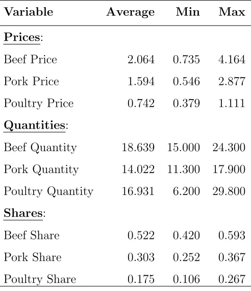
expenditures on chicken and turkey. Basic descriptive statistics for the meat data used in
all subsequent econometric analyses are reported in Table 1.
5.2
AIDS and Translog Estimates of US Meat Demand
The data and procedures described above are used to obtain meat demand estimates for
(log TL) version described in Section 3. We do this in part because in the present case the
log TL contains exactly the same number of free parameters as does the AIDS model and
therefore straightforward comparisons between the two specifications are facilitated. Prior to
estimation, all quantity variables and total expenditure are normalized to have a mean of one.
In both instances Holt’s (1998) first–order vector autoregressive autocorrelation procedure,
as described in Section 4.5, is used to handle issues with remaining serial correlation in
the models’ residuals. As well, because quarterly data are employed, and because there is
substantial seasonal patterns for some of these variables, most notably for quantities, a set
of seasonal dummy variables is appended to each model.
The final specification for the AIDS demand system is therefore:
wit=αi+αi1D1∗t +αi2D2∗t +αi3D3∗t +
X j
γijlnpjt+βi(ln(yt)−ln(Pt)) +eit, (31)
wherei=1 (Beef), 2 (Pork), and 3 (Poultry), and also wherelnPt is the price index give by
lnPt = X
k
(αk+αk1D1∗t +αk2D2∗t +αk3D3∗t) ln(pkt) +
1 2
X k
X j
γkjlnpktlnpjt. (32)
In addition to the restrictions defined in 6, the additional restrictions P3
j=1αjk = 0, k =
1,2,3 are required to ensure that adding–up holds. In (31)D1∗
t, D2∗t, and D3∗t are quarterly
dummy variables defined such that DJ∗
t =DJt−D4t, J = 1,2,3, and where DJt is one for
quarter J and zero otherwise. This dummy variable specification is used because it allows
the intercept term, in this case, αi to retain its original interpretation. See, for example,
van Dijk, Strikhom, and Ter¨asvirta (2003). Also note that in (32) we have restricted the
intercept term α0 to zero, a common practice in estimation of the AIDS model. 1
1
Empirical experience with the AIDS model has suggested that the likelihood function tends to be quite flat with respect to the α0 term, thus complicating estimation. One common practice is to evaluate the
Likewise, the final specification for the log TL model, corresponding to (13), is
wit =
αi+αi1D1∗t +αi2D2∗t +αi3D3∗t +
P
kγikln(pkt/yt)
−1 +P
kγM kln(pkt/yt)
+et, (33)
where again i =1 (Beef), 2 (Pork), and 3 (Poultry) and where γM k =PMi=1γik, M = 3. As
before the restrictionsP3
j=1αjk = 0, k = 1,2,3 are required to ensure that adding–up holds
for the share equations in (33). Finally, and in keeping with the log TL specification, the
additional restriction P
kγM k = 0 is imposed in estimation.
The parameter estimates for both models are reported in Table 2. Along with
parame-ter estimates and asymptotic standard errors, 90–percent bootstrapped confidence inparame-tervals
for the estimated parameters are obtained by using the percentile–t method. Specifically,
each parameter’s t–statistic is used to obtain critical values for the usual t–statistic as an
alternative to those provided by asymptotic theory. Empirically derived critical values are
then used to construct 90–percent confidence intervals for each estimated parameter. In
implementing the bootstrap 1,000 dynamic bootstrap draws are used to build the empirical
distribution for each parameter.
Because it is difficult to directly interpret many of the estimated parameters in the AIDS
and log TL models, it is generally more useful to obtain elasticity estimates. Results in
Table 2 do indicate that (1) seasonality is a significant feature in meat consumption; and
(2) serial correlation is a relevant feature of each model’s estimated residuals. Regarding
the latter, for both estimated models the dominant root for the estimated autocovariance
matrix is real-valued and is slightly less than one.
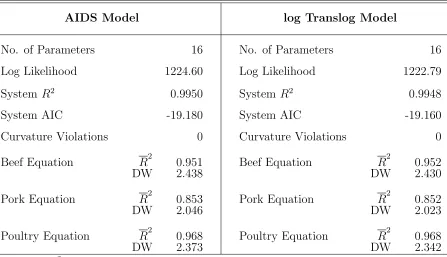
System and individual equation measures of fit and performance are recorded in Table
3. As previously noted both models have the same number of free parameters (16). The
estimated likelihood function value is slightly higher for the AIDS than for the log TL
implying, of course, that the AIC is slightly lower for the AIDS. Even so, the systemR2
values
to be negative semi–definite at all data points for both models, a result that is somewhat
surprising given the rather long time span used in estimation. Individually, each share
equation for each estimated model appears to fit the data well, as indicated by individual
equationR2
’s, with the pork equation apparently fitting most poorly of the three (R2
values
of 0.85). Overall, both the AIDS and log TL models provide a good fit to the data and,
moreover, both models provide a nearly identical fit to the data.
To obtain further insights into the implications of each estimated model for meat
con-sumption, Marshallian, Hicksian, and expenditure elasticities are obtained by using the
vari-ous formulae outlined in Sections 2 and 3. Elasticity estimates for the AIDS model, obtained
at the means of the sample data, are reported in Table 4, while the comparable estimates
for the log TL model are recorded in Table 5. As with parameter estimates, 90–percent
bootstrapped confidence intervals are provided for each elasticity estimate.
The elasticity estimates recorded in Tables 4 and 5 are consistent with those reported
elsewhere in the literature. See, for example, Piggott and Marsh (2004). Even so, several
observations are in order. To begin, qualitatively the price and expenditure elasticity
esti-mates are similar to each other for both models, which is perhaps not surprising given that
both models have the same number of parameters and that both fit the data equally well.
As well, all Marshallian own–price elasticity estimates are generally less than one in absolute
terms, the sole exception being pork for the AIDS model. Moreover, both models imply that
poultry demand is most inelastic—the point estimate of the Marshallian own–price elasticity
estimate for the AIDS model is -0.370 while the comparable estimate for the log TL model
is -0.474. In any event, neither model generates an own–price elasticity estimate for poultry
that is significantly different from zero, as implied by the 90–percent confidence intervals.
Indeed, the only price effect that is significantly different from zero for poultry demand is
that for beef.
Regarding the expenditure elasticities, the AIDS model implies an expenditure elasticity
estimate for the log TL model is 1.084, which is not significantly different from one. Indeed,
results in Table 5 reveal that none of the estimated expenditure elasticities is significantly
different from one, implying that consumer preferences are consistent with a homothetic
ordering. Indeed, this is the principle difference between the AIDS and the log TL models:
the log TL model seems to imply expenditure elasticity estimates for meat demand that are
consistent with homothetic preferences while the AIDS model does not.
6
Concluding Remarks
The AIDS and TL demand systems introduced by, respectively, Deaton and Muellbauer
(1980) and Christensen, Jorgenson, and Lau (1975) have over the past two–three decades
become primary workhorses in modern empirical demand analysis. Many refinements have
been considered for both specifications, including ways of incorporating demographic effects,
quadratic income terms, methods by which curvature conditions can be imposed, and issues
associated with incorporating structural change and seasonal effects. We also review
meth-ods for adjusting for autocorrelation in the model’s residuals. Finally, we present a set of
empirical examples for the AIDS and a the log TL version of the translog based on historical
meat price and consumption data for the United States. Because the properties of these
models are now well understood and because they are relatively easy to implement, there is
every reason to believe that the AIDS and TL demand systems, and the AIDS in particular,
References
Anderson, G. J., and R. W. Blundell (1982): “Estimation and Hypothesis Testing in Dynamic Singular Equation Systems,” Econometrica, 50, 1559–1571.
Attfield, C. L. F. (1997): “Estimating A Cointegrating Demand System,” Europen Economic Review, 41, 61–73.
Banks, J., R. Blundell, and A. Lewbel (1997): “Quadratic Engel Curves and Con-sumer Demand,” The Review of Economics and Statistics, 79(4), 527–539.
Barten, A. P.(1969): “Maximum Likelihood Estimatiion of a Complete System of Demand Equations,” Europen Economic Review, 1, 7–63.
Barten, A. P., and E. Geyskens (1975): “The Negaticity Condition in Consumer De-mand,” European Economic Review, 6, 227–260.
Berndt, E. R., and N. E. Savin(1975): “Estimation and Hypothesis Testing in Singular Equation Systems with Autoregressive Disturbances,” Econometrica, 43, 937–957.
Browning, M., and C. Meghir (1991): “The Effects of Male and Female Labor Supply on Commodity Demands,” Econometrica, 59(4), 925–951.
Buse, A. (1998): “Testing Homogeneity in the Linearized Almost Ideal Demand System,” American Journal of Agricultural Economics, 80(1), 208–220.
Chalfant, J. A.(1987): “A Globally Flexible, Almost Ideal Demand System,” Journal of Business and Economic Statistics, 5(2), 233–242.
Chalfant, J. A., R. S. Gray, and K. J. White (1991): “Evaluating Prior Beliefs in a Demand System: The Case of Meat Demand in Canada,” American Journal of Agricultural Economics, 73(2), 476–490.
Christensen, L., and M. E. Manser (1977): “Estimating U.S. Consumer Preferences for Meat with a Flexible Utility Function,” Journal of Econometrrics, 5, 37–53.
Christensen, L. R., D. W. Jorgenson, and L. J. Lau (1975): “Transcendental Log-arithmic Utility Functions,” The American Economic Review, 65(3), 367–383.
Davidson, J., and T. Ter¨asvirta (2002): “Long Memory and Nonlinear Time Series,” Journal of Econometrics, 110, 105–112.
Deaton, A., and J. Muellbauer (1980): “An Almost Ideal Demand System,” American Economic Review, 70(3), 312–326.
Deaton, A.,and J. Muellbauer(1980): Economics and Consumer Behavior. Cambridge University Press.
(1988b): “A Normalized Quadratic Semiflexible Functional Form,” Journal of Econometrics, 37, 327–342.
Eales, J. S., and L. J. Unnevehr (1988): “Demand for Beef and Chicken Products: Separability and Structural Change,” American Journal of Agricultural Economics, 70(3), 521–532.
(1994): “The Inverse Almost Ideal Demand System,” European Economic Review, 38(1), 101 – 115.
Gallant, A. R. (1981): “On the Bias in Flexible Functional Forms and an Essentially Unbiased Form: The Fourier Flexible Form,” Journal of Econometrics, 15(2), 211 – 245.
Gallant, A. R., and G. H. Golub(1984): “Imposing Curvature Restrictions on Flexible Functional Forms,” Journal of Econometrics, 26, 295–321.
Geweke, J. (1993): “Bayesian Treatment of the Independent Student-t Linear Model,” Journal of Applied Econometrics, 8, S19–S40.
Holt, M. T. (1998): “Autocorrelation Specification in Singular Equation Systems: A Further Look,” Economics Letters, 58, 135–141.
(2002): “Inverse Demand Systems and Choice of Functional Form,” European Economic Review, 46, 117–142.
Hotelling, H. (1935): “Demand Functions with Limited Budgets,” Econometrica, 3(1), 66–78.
Karagiannisa, G., and G. J. Mergos (2002): “Estimating Theoretically Consistent Demand Systems Using Cointegration Techniques with Application to Greek Food Data,” Economics Letters, 74, 137–143.
Lafrance, J. T. (2004): “Integrability of the Linear Approximate Almost Ideal Demand System,” Economics Letters, 84, 297–303.
Lewbel, A. (1989): “Nesting the Aids and Translog Demand Systems,” International Economic Review, 30(2), 349–356.
Lewbell, A., and S. Ng(2005): “Demand Systems with Nonstationary Prices,” Review of Economics and Statistics, 87, 479–494.
Moschini, G. (1995): “Units of Measurement and the Stone Index in Demand System Estimation,” American Journal of Agricultural Economics, 77, 63–68.
(1998): “The Semiflexible Almost Ideal Demand System,” European Economic Review, 42, 349–364.
Moschini, G., and K. D. Mielke (1989): “Modelling the Pattern of Structural Change in U.S. Meat Demand,” American Journal of Agricultural Economics, 71, 253–261.
Moschini, G., and D. Moro(1994): “Autocorrelation Specification in Singular Equation Systems,” Economics Letters, 46, 303–309.
Ng, S. (1995): “Testing for Homogeneity in Demand Systems When the Regressors Are Non-stationary,” Journal of Applied Econometrics, 10, 147–163.
Piggott, N. E., and T. L. Marsh(2004): “Does Food Safety Information Impact U.S. Meat Demand?,” American Journal of Agricultural Economics, 86, 154–174.
Pollak, R. A., and T. J. Wales(1992): Demand System Specification and Estimation. Oxford University Press.
Ryan, D. L., andT. J. Wales(1998): “A Simple Method for Imposing Local Curvature in some Flexible Consumer–Demand Systems,” Journal of Business and Economic Statistics, 16, 331–338.
Terrell, D. (1996): “Incorporating Monotonicity and Concavity Conditions in Flexible Functional Forms,” Journal of Applied Econometrics, 11(2), 179–194.
U.S. Department of Agriculture(2006a): “Economic Resaerch Service. Poultry Year-book,” Online, Stock No. 89007.
(2006b): “Economic Research Service. Red Meat Yearbook,” Online Publication, Stock No. 94006.
Table 1: Descriptive Statistics for Meat Demand Variables, 1960–2004.
Variable Average Min Max
Prices:
Beef Price 2.064 0.735 4.164
Pork Price 1.594 0.546 2.877
Poultry Price 0.742 0.379 1.111
Quantities:
Beef Quantity 18.639 15.000 24.300
Pork Quantity 14.022 11.300 17.900
Poultry Quantity 16.931 6.200 29.800
Shares:
Beef Share 0.522 0.420 0.593
Pork Share 0.303 0.252 0.367
Poultry Share 0.175 0.106 0.267
[image:28.612.184.430.119.404.2]Table 2: AIDS and log Translog Model Parameter Estimates for Quarterly U.S. Meat Demand with Seasonal Dummy Variables and Autocorrelation Corrections, 1960–2004.
AIDS Model Parameter Estimates log Translog Model Parameter Estimates
Asy. Asy.
Parameter Estimate Std. Error 90% CI Parameter Estimate Std. Error 90% CI
α1 0.461 0.067 [ 0.359 0.839] α1 -0.445 0.090 [-1.070 -0.318]
α11 0.004 0.001 [ 0.002 0.005] α11 -0.003 0.001 [-0.004 -0.001]
α12 0.011 0.001 [ 0.009 0.013] α12 -0.010 0.001 [-0.012 -0.009]
α13 0.008 0.001 [ 0.006 0.009] α13 -0.008 0.001 [-0.009 -0.006]
γ11 0.074 0.020 [ 0.041 0.108] α2 -0.271 0.034 [-0.453 -0.218]
γ12 0.027 0.015 [-0.001 0.055] α21 -0.008 0.001 [-0.009 -0.006]
β1 0.020 0.030 [-0.031 0.070] α22 0.010 0.001 [ 0.009 0.012]
α2 0.274 0.029 [ 0.231 0.400] α23 0.010 0.001 [ 0.008 0.011]
α21 0.008 0.001 [ 0.007 0.010] γ11 -0.094 0.038 [-0.157 -0.038]
α22 -0.010 0.001 [-0.011 -0.008] γ12 -0.032 0.020 [-0.065 -0.002]
α23 -0.010 0.001 [-0.011 -0.008] γ13 0.109 0.019 [ 0.079 0.139]
γ22 0.010 0.019 [-0.022 0.043] γ22 -0.007 0.023 [-0.041 0.027]
β2 0.041 0.030 [-0.003 0.089] γ23 0.036 0.016 [ 0.008 0.064]
τ11 0.783 0.010 [ 0.766 0.794] τ11 0.780 0.010 [ 0.764 0.792]
τ12 -0.344 0.021 [-0.375 -0.299] τ12 -0.334 0.020 [-0.368 -0.290]
τ22 0.680 0.009 [ 0.665 0.690] τ22 0.674 0.011 [ 0.657 0.686]
Note: Asymptotic standard errors are in columns headed Asy. Std. Error. Columns titled ‘90% CI’ contain 90–percent bootstrapped confidence intervals obtained by using the percentile t method over 1000 bootstrap draws. The poultry equation is omitted during estimation. Sample size is T = 179.
Table 3: Measures of Fit for Estimated AIDS and log Translog Models.
AIDS Model log Translog Model
No. of Parameters 16 No. of Parameters 16
Log Likelihood 1224.60 Log Likelihood 1222.79
System R2
0.9950 System R2
0.9948
System AIC -19.180 System AIC -19.160
Curvature Violations 0 Curvature Violations 0
Beef Equation R2 0.951 Beef Equation R2 0.952
DW 2.438 DW 2.430
Pork Equation R2 0.853 Pork Equation R2 0.852
DW 2.046 DW 2.023
Poultry Equation R2 0.968 Poultry Equation R2 0.968
DW 2.373 DW 2.342
Table 4: Estimated Marshallian, Expenditure, and Hicksian Elasticities for the Es-timated AIDS Model.
Marshallian Price Elasticities Expenditure Elasticities
Beef Pork Poultry
Beef -0.868 0.044 -0.217 Beef 1.041
[-0.783 -0.954] [-0.020 0.095] [-0.142 -0.255] [0.948 1.126]
Pork 0.026 -1.004 -0.172 Pork 1.150
[-0.100 0.150] [-0.897 -1.113] [-0.056 -0.234] [0.993 1.280]
Poultry -0.296 -0.084 -0.370 Poultry 0.750
[-0.184 -0.639] [-0.266 0.073] [-0.506 0.163] [0.365 0.929]
Hicksian Price Elasticities
Beef Pork Poultry
Beef -0.360 0.326 0.035
[-0.270 -0.410] [0.297 0.405] [-0.080 0.049]
Pork 0.586 -0.692 0.106
[0.511 0.704] [-0.571 -0.785] [-0.033 0.167]
Poultry 0.070 0.119 -0.189
[-0.260 0.139] [-0.077 0.235] [-0.287 0.281]
Note: Numbers in box brackets are 90–percent bootstrapped confidence intervals. All elas-ticities are computed at the means of the sample data.
Table 5: Estimated Marshallian, Expenditure, and Hicksian Elasticities for the Es-timated log Translog Model.
Marshallian Price Elasticities Expenditure Elasticities
Beef Pork Poultry
Beef -0.823 0.063 -0.204 Beef 0.965
[-0.753 -0.903] [0.005 0.110] [-0.127 -0.250] [0.882 1.053]
Pork 0.102 -0.976 -0.113 Pork 0.987
[-0.022 0.205] [-0.886 -1.093] [-0.011 -0.187] [0.856 1.142]
Poultry -0.460 -0.150 -0.474 Poultry 1.084
[-0.357 -0.918] [-0.052 -0.369] [-0.597 0.059] [0.853 1.362]
Hicksian Price Elasticities
Beef Pork Poultry
Beef -0.356 0.323 0.033
[-0.268 -0.409] [0.296 0.399] [-0.075 0.053]
Pork 0.580 -0.710 0.130
[0.509 0.695] [-0.579 -0.789] [-0.012 0.182]
Poultry 0.065 0.142 -0.207
[-0.287 0.135] [-0.003 0.270] [-0.326 0.222]
Note: Numbers in box brackets are 90–percent bootstrapped confidence intervals. All elas-ticities are computed at the means of the sample data.