Munich Personal RePEc Archive
EPL and Job Contract Conversion Rate:
The Italian CFL Case
Grassi, Emanuele
University of Salento
January 2009
EPL and job contract conversion rate:
The Italian CFL case
Emanuele Grassi
Department of Economics, Mathematics and Statistics
University of Salento
November 30, 2008
Abstract
1
Introduction
It is well known that …rms often need to carry out screening procedures to evaluate workers’ skill levels before stabilizing the …rm-worker job relation-ship, and it might also be costly for them to dismiss workers once they are hired. As long as …rms cannot make use of any speci…c tool to evaluate some of the applicants’ characteristics - i.e. practical skills, cooperative attitudes - their choice could be ine¢cient because after a worker is hired and her unsuitability for the job is understood, a …rm has an incentive to dismiss the worker. But since Employment Protection Legislation (EPL) usually poses some costs on this choice, …rms might be obliged to keep a worker even though her/his unsuitability1. This in turn implies the presence of ine¢ciencies and
frictions in …rms’ hiring procedures.
Cahuc and Postel-Vinay (2002) state that because of higher …ring costs, the conversion rate of temporary contracts into long-term contracts should simply drop. Following this reasoning, in the long run we should observe that …rms subject to EPL should progressively convert all the workforce into a temporary one. But in reality, …rms tend to keep a stable workforce even if EPL is enforced. This behavior can be compatible with economic incen-tives, in fact if workers need to be trained for speci…c tasks, …rms might not be willing to iterate training activities each time they dismiss their tempo-rary workforce. It might also be the case that …rms want to retain certain workers because of their skills. Moreover, high turnover rates could be an incentive for temporary workers to exert less e¤ort, and this in turn implies detrimental e¤ects in terms of …rm-level productivity. Finally, it could be too costly for …rms to keep un…lled jobs each time a contract comes to its expiration. So, given that …rms could also be interested in retaining some workers, higher EPL could also push …rms to be more aware of the "screening side" of temporary contracts. Thus, EPL could result in a higher conversion
rate of …xed-term contracts into open-ended ones.
The research question which underlies this paper is thus to shed some light on the causal e¤ect of dismissal costs on the conversion of temporary contracts into permanent ones in the same …rm. To …nd empirical evidence of this relationship, I study the e¤ect of the Italian 1990 reform - which introduced unjust dismissal costs for small …rms - on the conversion rate of theContratto di Formazione e Lavoro (working and training contract - CFL) into permanent contracts.
The rest of the paper is organized as follows. Section 2 considers the branch of the literature which this study is nested to. Section 3 describes the CFL program. Section 4 is devoted to the empirical analysis. Section 5 concludes.
2
EPL: some theoretical and empirical
ad-vances
Employment Protection Legislation (EPL) is a widely investigated institu-tional feature of labour markets and consists of a set of rules according to which the …rms’ hiring and …ring processes are regulated. In particular, EPL de…nes conditions to be complied with by employers in case of fair and un-fair layo¤s2. In case of individual dismissal, EPL prescribes advance notice
periods, third parties’ roles (for example prior negotiation with trade unions or administrative authorizations), procedures to challenge the layo¤ decision, and possible severance payments3. Despite they are intended to promote
em-ployment stability, their actual e¤ects are at the centre of an intense debate, and, in the last two decades, the work of many economists has been of great help in exploring several dimensions of the impact of EPL reforms on labour
2Fair layo¤s are justi…ed by disciplinary or economic reasons, while unfair layo¤s can
be brought about by several reasons, such as discriminatory practices.
market outcomes.
From a theoretical point of view, EPL is thought to be a source of distor-tion of labour market outcomes as long as it a¤ects …rms’ employment choices and workers’ behavior. Matching models with endogenous job creation and destruction in the spirit of Mortensen and Pissarides (1994) predict an am-biguous e¤ect on the (un)employment rate. Garibaldi (1998) comes to similar conclusions by extending search models to analyze the cyclical behavior of job reallocation. Asymmetric responses of job creation and job destruction are closely related to the nature of …ring permissions. Continuously avail-able …ring permissions makes job reallocation countercyclical, but when …ring permissions are time consuming, the asymmetry disappears. Garibaldi and Pacelli (2008) focus on the e¤ect of severance payments on job separation. They look at the Italian labour market and use a deferred wage scheme - the
Trattamento di Fine Rapporto - to give empirical content to the theoretical prediction that an increase in severance payments increases labour hoarding. Indeed, they …nd that a 60% advance withdrawals of accumulated wages in-crease the probability of separation by roughly 20%. Lazear (1990) shows that in a perfect labour market, EPL has no real e¤ects on employment, while transfers from workers to …rms (formalized through properly designed labour contracts) alter the workers’ wage-tenure pro…le. Leonardi and Pica (2007) give empirical content to this proposition. Indeed, they …nd a decrease of the returns to tenure by 20% in the …rst year and by 8% over the …rst two years.
after the reform as well as a closing gap of …rms ‡ows after the reform. Their …ndings suggest that heavier EPL reduces ‡ows into and out of employment, but with negligible e¤ects on net employment. They also …nd that after the reform small …rms were less likely to enter the market. Ichino and Riphahn (2005) explore the e¤ect of EPL on workers’ behavior in terms of absenteeism as a measure of worker e¤ort. They use data on white-collar workers from a large Italian bank, and exploit the presence of the institution of probation to check whether more employment protection alters the average number of days of absence from work. They …nd that after twelve weeks of probation (a period etablished by law), new hired workers tend to be more absent. More recently, Bassanini et al. (2008) empirically investigate the impact of EPL on productivity in the OECD. The authors provide some evidence of the nega-tive impact of dismissal regulations on TFP growth, and identify the channel through which it operates. In particular they …nd that changes in labour composition due to stricter EPL do not play any speci…c role, while layo¤ restrictions alter the e¢ciency improvements and the technological change, thus the productivity.
3
The Italian
Contratto di Formazione e
La-voro
Before the introduction of the working and training contract, Italian …rms could hire either on a permanent basis or through apprenticeship contracts4.
Employment agencies (u¢ci di collocamento) played a substantial monopo-listic role. Thus, CFLs can be viewed as one of the …rst attempts at intro-ducing ‡exibility in the labour market. Despite the success of the program over the subsequent years, only few studies have been speci…cally devoted to
4The apprenticeship contract has been introduced in 1959 to provide young people
the analysis of this program5.
The Contratto di Formazione e Lavoro (working and training contract) has been introduced in 1985 in order to tackle with the high unemployment rate among young workers. Initially, the program was targeted to people aged 15 to 29 and it was expected to increase the chance to get a job and to improve human capital accumulation among young workers. Indeed, the program established compulsory training activities (o¤-the-job training) be-side working tasks (on-the-job training and learning by doing). Firms were encouraged to make use of this contract and to provide some forms of train-ing through a structure of incentives, such as the reduction of Social Security fees. The CFL was thought as a …xed term contract, in fact it could not last more than two years and was not renewable. Moreover it could not be con-verted into an open ended contract before 18 months. After the 18th month and before the expiration of the contract, the …rm had the option either to hire the worker on a permanent basis or to dismiss her/him without incurring in any separation cost. As already pointed out, to increase workers’ future employability, the CFL included a compulsory training period, but it seems that this feature has remained mostly unheard6. Moreover, the program has
been implementedat the margin introducing some forms of ‡exibility, in fact it was not targeted to existing workers.
Firms’ pro…tability at using working and training contracts was twofold. First, …rms could adjust the labor force at a lower cost in response to speci…c production needs. In this case, …rms did not have any incentive to provide any form of stable training, because it was not convenient to share the cost of training if they knew that they were not able to exploit the potential bene…ts coming from the higher level of skills acquired by the worker. Thus, if this was the main goal that …rms pursued when recruiting young workers, they
5Contini, Cornaglia, Malpede and Rettore (2002) and Tattara and Valentini (2005)
explore the implications of the programme on the short- and long-term chances to get a job; Contini and Revelli (2004) perform a welfare analysis of the program.
were frustrating the incentive scheme of the CFL program. Second, …rms could use these contracts as a screening device through which they could select high ability young workers according to their skill requirement needs. In this case, when …rms’ skill requirements were met, part of the working and training contracts could be converted into permanent ones.
period 1988 to 1994 and compare it with the behavior of large …rms.
My research question is relevant at least for two reasons. First it shows that a proper evaluation of Active Labour Market Policies must take into account institutional features, such as EPL. Second, after the di¤usion of …xed term contracts in European countries, a key problem is to establish to what extent these contracts represents a stepping stone or a dead end to per-manent employment. As shown by Gagliarducci (2005), repeated temporary jobs can be detrimental to workers future performances in terms of labour market outcomes, thus it is interesting to look at the conversion rate of job contracts within the same …rm as an important aspect of policy e¤ectiveness.
4
Dismissal costs and job contract conversion
rates
4.1
Identi…cation strategy.
In order to identify the causal e¤ect of dismissal costs on the job contract conversion rate, I employ a di¤erence-in-di¤erences strategy (DID). The DID design takes full advantage of the natural experiment set up yielded by the 1990 reform. As a result, individuals belong either to small businesses or large ones and are observed either before or after the reform. In particular, individuals are indexed with theisubscript and belong to one of the mutually excluded groups, i 2 f0;1g, where i = 0refers to being employed in a large
…rm and i = 1refers to being employed in a small …rm. The …rst group is the
control group (or untreated group), while the second is the treatment group. I consider two independent cross sections, thus each individual is observed only once, either before(t=b)or after(t =a)the treatment. De…ne i 1[t=a],
where 1[ ] is the indicator function. Thus i = 0 if the i th individual is
observed before the treatment and i = 1 if the i th individual is observed
into permanent contracts (in the same …rm) and can take values equal to0or
1. Lety0
i be the potential outcome for thei th individual when she does not
receive the treatment, andy1
i be the potential outcome for an individual when
she does receive the treatment. Furthermore, let di = i i be the indicator
of the treatment status, so di = 1 means that an individual is employed in
a small …rm after the treatment. What is observed is the triple (yi; i; i),
where i = (1 i) ib+ i ia, and the actual outcome for individualiis equal
to7
yi = (1 i)yib0 + i[(1 i)yia0 + iy1ia] (1)
The standard di¤erence-in-di¤erences formula is:
AT T = E ya1j a = 1; = 1 E y0bj b = 1; = 0 (2) E y0
aj = 0; = 1 E y
0
bj = 0; = 0 =DID
For the identi…cation of the treatment e¤ect on the treatedAT T E(y1
a y0
aj a= 1), we need the following three conditions to hold8:
Condition 1 E(y0
a yb0j a = 1) =E(ya0 yb0j a = 0)
Condition 2 E(y0
bj b = 0) = E(y0bj a = 0) and E(yb0j b = 1) = E(yb0j a =
1)
Condition 3 is mean independent of ytj given t for all j = 0;1 and t =b; a.
The …rst condition states that if a di¤erence in the outcome between groups exists, it must be constant over time. If several cross sections were available, the assumption would become a testable one, but in this study this
7See Lee (2005).
is not possible for at least two reasons: …rst the time dimension has been re-duced in order to avoid the overlap of di¤erent policies; second, since CFLs last no more than two years, it would be problematic to built subsequent waves, because in each year there could be workers belongig from di¤erent waves. To indirectly check the validity of the assumption, I rely on four dif-ferent subsamples aimed to make the treatment and control groups as similar as possible. In a …rst subsample, I restrict the control group to individuals belonging to …rms with no more than 50 employees. This should reduce considerably any unobserved di¤erences between treated and control units in terms of their time-varying responses to business cycle ‡uctuations. The remaining three subsamples are built by following a propensity score overlap
criteria. I exclude from the original sample those observations whose propen-sity score lies in the tails of the distributions according to three thresholds, 5%, 10% and 15%9.
Di¤erently from the …rst identifying condition, conditions 2 and 3 are directly testable. These conditions state that the groups composition must be constant over time, otherwise there would be four di¤erent subpopulations which would not be informative to extrapolate any causal e¤ect from the data. In practice, if the two conditions are not violated, any systematic move between groups is ruled out, and this makes the groups comparable. Section 4.3 is devoted to this analysis.
The baseline speci…cation used to estimate the e¤ect of EPL on job con-tract conversion rates is:
E yjij i; di = 0 + i+ t+ ddi (3)
where the dependent variable yji is a binary variable which is equal to 1 every time a working and training contract is converted into a permanent one in the same …rm and 0 otherwise. i is a dummy which takes the value of
9The Appendix provides a detailed description about the procedure used to estimate
1 whenever a worker is employed in a …rm with less than 15 employees; t is
the dummy variable which takes the value of 1 for those individuals observed after 1990; di is a dummy which takes the value of 1 if an individual is
observed after the reform in a small business and is intended to capture the e¤ect of the policy change. To control for the possibility that the change in the outcome is driven by the change in workers’ and …rms’ characteristics, I include a set of covariates which are aimed at relieving this potentially source of bias. The estimated model is thus:
E yjij i; di; xi = 0+ i+ t+ ddi+ 0xxi (4)
wherexi is a vector of workers and …rms characteristics, including gender,
age, occupation, (log) daily wage, economic sectors, …rm’s age and average …rm size. To control for spacial di¤erences, I also include regional dummies in separate regressions, as well as interaction terms.
Since the Linear Probability Model has many potentially drawbacks, i.e. the predicted probabilities might not lie in the 0-1 interval, it is convenient to rely on an explicit Cumulative Distribution Function. In particular, I conduct probit estimates for all the speci…cations already outlined and for all the subsamples.
4.2
The dataset and preliminary analysis
To empirically test my research question, I use the Work Histories Italian Panel (WHIP)10. The dataset is a 1:90 random sample drawn from the Italian
Social Security Administration (INPS) collecting information on employees in private …rms on an annual basis. From the original data, I build two independent cross sections, one referring to the pre-reform period and the
10WHIP–Work Histories Italian Panel–Full Edition, work histories on Social Security
other referring to the post-reform period11. In both cases I select workers
hired under working and training contracts and follow them up to their …rst transition in a di¤erent labour status. I end up with two waves, the …rst includes 3328 observations (with 48.32% employed in small …rms, and 51.68% in large …rms), while the second is made up of 2997 observations (with 49.85% employed in small …rms, and 50.15% in large …rms). Since the maximum contract length could never exceed two years, I start following workers since 1987 and 1991. In this way, those who begun working in 1987 have been followed up to 1989, and, similarly, those who begun working in 1991 have been followed up to 199312. For each worker, I observe the …rst transition
out of the CFL status. I exploit the fact that the WHIP is a linked employer-employee dataset, so it is possible to know whether or not the subsequent job was in the same …rm and under a permanent position. Every time a CFL is converted into a permanent contract in the same …rm, the dependent variable takes the value of 1. For each worker, the dataset provides information on individual characteristics - gender, age, daily wage and worker/employee status- and on …rm’s characteristics - …rm’s age, economic sector, average …rm size and localization on a regional basis13.
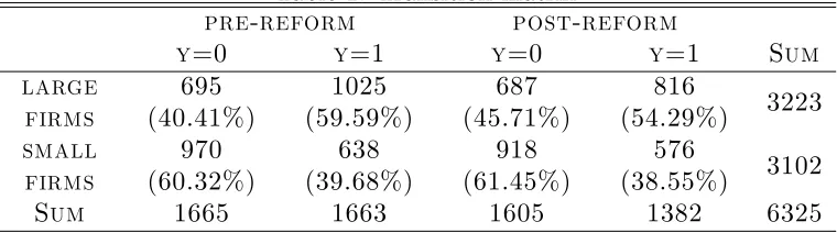
Table 1 reports the number and percentages of observations for each time period and for control and treatment groups. Note that 1494 individuals were exposed to the treatment. The table also shows the number of transitions into permanent contracts in the same …rm by …rms’ type and for both periods. With respect to the pre-reform period, the total number of CFL signed in 1991 declines both for large …rms (-12.62%) and small …rms (-7.09%). While
11This choice is driven by the fact that I need to cover a period as homogenous as
possible in terms of the underlying legislation.
12This choice allows me to get a pre-reform wave which is totally una¤ected by the 1990
reform because the last job contract conversion happens to be in 1989. Furthermore, by selecting the 1991 wave, I avoid taking into account intermediate waves (i.e. the 1989 wave) because the reform might not fully have exerted its e¤ects on them.
13One limit of this study is that few information is available about individuals
for small businesses the proportion of conversions (y= 1) is almost the same in the two periods, for large businesses there is an evident decline in the conversion rate of CFL into permanent contracts.
Table 1: Transition matrix
pre-reform post-reform
y=0 y=1 y=0 y=1 Sum
large firms 695 (40.41%) 1025 (59.59%) 687 (45.71%) 816 (54.29%) 3223 small firms 970 (60.32%) 638 (39.68%) 918 (61.45%) 576 (38.55%) 3102
Sum 1665 1663 1605 1382 6325
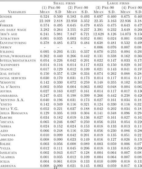
Table 2 shows descriptive statistics by …rm size, before and after the 1990 reform. Large …rms are systematically older than small businesses, employ less women and pay slightly higher wages. Small …rms are absent from the energy sector and are less present in the manufacturing sector, while they are more present as retailers and wholesalers.
4.3
Assessing the balance of covariate distributions
Table 2: Individual descriptive statistics (full sample)
Small firms Large firms
(1) Pre-90 (2) Post-90 (3) Pre-90 (4) Post-90
Variables Mean S.D Mean S.D. Mean S.D. Mean S.D.
Gender 0.524 0.500 0.583 0.493 0.697 0.460 0.675 0.469
Age 22.169 2.818 22.950 3.352 22.35 3.163 22.936 3.184
Worker 0.574 0.495 0.645 0.479 0.655 0.475 0.643 0.479
Log daily wage 3.282 0.264 3.555 0.237 3.391 0.232 3.649 0.260
Firm’s age 6.241 5.981 7.847 6.721 12.628 8.126 14.073 9.150
Extraction 0.001 0.035 0.003 0.052 0.001 0.024 0.001 0.036
Manufacturing 0.378 0.485 0.373 0.484 0.638 0.481 0.532 0.499
Energy - - - - 0.006 0.076 0.007 0.081
Building 0.095 0.293 0.131 0.337 0.070 0.255 0.094 0.293
Retail/wholesale 0.262 0.440 0.266 0.442 0.131 0.338 0.162 0.368
Hotels/restaurants 0.054 0.226 0.042 0.201 0.022 0.147 0.033 0.178
Transports 0.014 0.116 0.014 0.117 0.023 0.150 0.029 0.167
Finance 0.017 0.129 0.012 0.109 0.021 0.143 0.041 0.197
Real estate 0.150 0.357 0.128 0.334 0.074 0.262 0.088 0.284
Social services 0.030 0.170 0.031 0.173 0.014 0.117 0.014 0.117
Piemonte 0.142 0.330 0.072 0.259 0.148 0.355 0.102 0.303
Val d’Aosta 0.002 0.050 0.004 0.063 0.002 0.048 0.004 0.063
Liguria 0.027 0.163 0.027 0.161 0.014 0.117 0.017 0.130
Lombardia 0.247 0.431 0.198 0.399 0.266 0.442 0.238 0.426
Trentino A.A. 0.040 0.196 0.031 0.173 0.027 0.161 0.034 0.181
Veneto 0.142 0.349 0.116 0.321 0.124 0.330 0.116 0.321
Friuli V.G. 0.052 0.221 0.037 0.188 0.042 0.202 0.034 0.181
Emilia Romagna 0.129 0.335 0.103 0.304 0.141 0.348 0.096 0.294
Marche 0.034 0.182 0.019 0.136 0.027 0.161 0.027 0.163
Toscana 0.065 0.246 0.067 0.250 0.056 0.231 0.054 0.226
Umbria 0.024 0.152 0.024 0.153 0.018 0.133 0.013 0.115
Lazio 0.066 0.248 0.116 0.320 0.056 0.230 0.086 0.280
Campania 0.010 0.099 0.042 0.201 0.019 0.135 0.051 0.221
Abruzzo 0.008 0.090 0.023 0.149 0.016 0.127 0.026 0.159
Molise 0.003 0.056 0.008 0.089 0.003 0.059 0.006 0.077
Puglia 0.012 0.111 0.045 0.206 0.018 0.133 0.045 0.206
Basilicata 0.002 0.043 0.017 0.128 0.004 0.064 0.007 0.081
data, we run into this situation in just one case, namely the energy sector14.
Moreover, even if there is enough overlap in covariate supports, the distri-butions might di¤er in their shape. Here I try to mimic the output of the "research design" phase by assessing the balance of covariate distributions. If su¢cient balance is there, then the control groups are more likely to have similar responsiveness to the underlying economic environment15. Moreover,
the estimates become more credible and inference is more robust because it is less likely that systematic di¤erences among groups’ characteristics bias the results.
The assessment of the balance in covariate distributions is carried out on a univariate basis through mean-comparison tests16, normalized di¤erences
in averages and di¤erences in log-standard deviations for each covariate. I also conduct a graphical analysis of the covariates’ distributions to capture any di¤erence which is not detected by the above mentioned analysis. In particular, I construct histograms for those variables presenting symptoms of imbalance17.
With a known univariate distribution, let call its …rst and second order moments, respectively, = E[Xj = ] and 2 = V [Xj = ], with =
t; cj - where t is for treated and cj is for the j th control group. The
univariate analysis will look at the following measures: i. 1 = t cj
ii. 2 =
t cj
q
2
t + 2cj
iii. = ln ( t) ln cj
14Note that by excluding the energy sector from the analysis, I only loose …ve
observa-tions.
15See Eissa and Liebman (1996).
16Every time the covariate under analysis is a dummy variable, a test of proportion is
carried out, while when the covariate is not binary, a standard t-test is performed.
To estimate these measures, a natural way is to use sample means and variances18. Let X
t and Xc the sample averages for treated and control
groups, with Xt =
1
Nt
P
i;Wi=t
Xi and Xcj =
1
Ncj
P
i;Wi=cj
Xi; where Nt is the
number of treated units and Ncj is the number of control units in group j. Moreover, let s2
t and s
2
cj the sample covariate variances, with s
2
t =
1
Nt 1
P
i;Wi=t
Xi Xt
2
and s2
cj =
1
Ncj 1
P
i;Wi=cj
Xi Xcj
2
. Thus, the sample counterparts of (i)-(iii) are:
i’. ^1 = Xt Xcj
ii’. ^2 =
Xt Xcj
q
s2
t +s2cj
iii’. ^ = ln (st) ln scj .
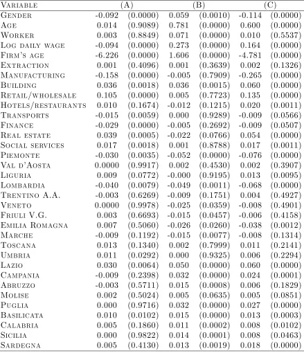
Formula (i’) has been used to compute mean comparison tests, and table 3 reports the p-values. Under the null hypothesis the group averages are equal, so we do not wish to reject the null hypothesis, since our hope is to …nd similar averages among treated and controls. Note that in the di¤erence-in-di¤erences set up, we have four groups, only one of them is the treated group (small …rms after the 1990 reform), while the others can be all thought of as control groups. Thus, I compare sample covariate averages for treated and control groups. In column (A), the control group is "large …rms after the reform"; in column (B) the control group is "small …rms before the reform"; in column (C) the control group is "large …rms before the reform". In each cell, I report the di¤erence in averages and the p-values in parentheses.
At a 10% level of signi…cance, we do not reject the null hypothesis of equal averages in 40 out of 102 cases; at a 5% level of signi…cance there are 46 cases in which I do not reject the null; while at a 1% level of signi…cance the cases are 53. Even though the percentage of rejections is always below
Table 3: Group average tests
Variable (A) (B) (C)
Gender -0.092 (0.0000) 0.059 (0.0010) -0.114 (0.0000)
Age 0.014 (0.9089) 0.781 (0.0000) 0.600 (0.0000)
Worker 0.003 (0.8849) 0.071 (0.0000) 0.010 (0.5537)
Log daily wage -0.094 (0.0000) 0.273 (0.0000) 0.164 (0.0000)
Firm’s age -6.226 (0.0000) 1.606 (0.0000) -4.781 (0.0000)
Extraction 0.001 (0.4096) 0.001 (0.3639) 0.002 (0.1326)
Manufacturing -0.158 (0.0000) -0.005 (0.7909) -0.265 (0.0000)
Building 0.036 (0.0018) 0.036 (0.0015) 0.060 (0.0000)
Retail/wholesale 0.105 (0.0000) 0.005 (0.7723) 0.135 (0.0000)
Hotels/restaurants 0.010 (0.1674) -0.012 (0.1215) 0.020 (0.0011)
Transports -0.015 (0.0059) 0.000 (0.9289) -0.009 (0.0566)
Finance -0.029 (0.0000) -0.005 (0.2692) -0.009 (0.0507)
Real estate 0.039 (0.0005) -0.022 (0.0766) 0.054 (0.0000)
Social services 0.017 (0.0018) 0.001 (0.8788) 0.017 (0.0011)
Piemonte -0.030 (0.0035) -0.052 (0.0000) -0.076 (0.0000)
Val d’Aosta 0.0000 (0.9917) 0.002 (0.4530) 0.002 (0.3907)
Liguria 0.009 (0.0772) -0.000 (0.9195) 0.013 (0.0095)
Lombardia -0.040 (0.0079) -0.049 (0.0011) -0.068 (0.0000)
Trentino A.A. -0.003 (0.6269) -0.009 (0.1751) 0.004 (0.4927)
Veneto 0.0000 (0.9978) -0.025 (0.0359) -0.008 (0.4901)
Friuli V.G. 0.003 (0.6693) -0.015 (0.0457) -0.006 (0.4158)
Emilia Romagna 0.007 (0.5060) -0.026 (0.0260) -0.038 (0.0012)
Marche -0.009 (0.1192) -0.015 (0.0077) -0.008 (0.1314)
Toscana 0.013 (0.1340) 0.002 (0.7999) 0.011 (0.2141)
Umbria 0.011 (0.0292) 0.000 (0.9325) 0.006 (0.2294)
Lazio 0.030 (0.0064) 0.050 (0.0000) 0.060 (0.0000)
Campania -0.009 (0.2398) 0.032 (0.0000) 0.024 (0.0001)
Abruzzo -0.003 (0.5711) 0.015 (0.0008) 0.006 (0.1829)
Molise 0.002 (0.5024) 0.005 (0.0635) 0.005 (0.0851)
Puglia 0.000 (0.9716) 0.032 (0.0000) 0.027 (0.0000)
Basilicata 0.010 (0.0102) 0.015 (0.0000) 0.013 (0.0003)
Calabria 0.005 (0.1860) 0.011 (0.0002) 0.008 (0.0102)
Sicilia 0.000 (0.9822) 0.014 (0.0001) 0.008 (0.0463)
52%, and many times the tests suggest unequal averages, the di¤erences do not seem to be drastically away from each other. In fact, even if the mean comparison test rejects the null hypothesis, the di¤erence in averages is often less than a standard deviation19. This suggests that it is important to use a
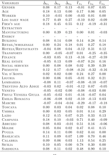
measure able to take into account the dispersion in covariate distributions. This check is shown in table 4 which reports the normalized di¤erences in averages20 (columns 2 to 4) and the di¤erences in log-standard deviations
(columns 5 to 7)21. From the inspection of columns 2 to 6, we can see that
there is overall balance among groups exept for two variables, namely the log daily wage and …rms age. This suggests that the full sample can be conveniently used as a starting point for the analysis, while more accurate estimates can be conducted on the subsamples already mentioned.
4.4
The e¤ects of the 1990 reform on CFL conversion
rates
Tables 5 and 6 show the DID results from OLS and probit estimates. Both tables report marginal e¤ects estimated on the full sample of CFL workers. Table 7 reports the results from probit estimates carried out on four di¤erent subsamples. Labels (S1)-(S4) refer to di¤erent speci…cations of the model: (S1) is the baseline speci…cation, (S2) adds workers’ and …rms’
characteris-19Here I refer to the standard deviations computed for the covariates of the treated
group.
20Note that the normalized di¤erence is a useful tool because it is a pure measure of
localization corrected by the square root of the sum of variances. An example might clarify this point. Suppose we have two cases both with a small di¤erence in means (inducing the reader to think that the situation is positive), but in the …rst case the variances are very low, while in the second are very large. If we do not correct for the variance, we are not able to detect the lack of overlap around the averages. In fact, when the two distributions are very concentrated, even a small di¤erence in means must be looked as a potential source of bias.
21The indexes refer to the comparison between treated (t) and one of the control groups:
c1is "small …rms before the reform",c2 is "large …rms before the reform" andc3is "large
Table 4: Normalized di¤erence in averages and di¤erences in the log-standard deviations
Variables ^tc1 ^tc2 ^tc3 ^tc1 ^tc2 ^tc3
Gender 0.08 0.17 0.13 -0.01 0.07 0.05
Age 0.18 0.13 0.00 0.17 0.06 0.05
Worker 0.10 -0.01 0.00 -0.03 0.01 0.00
Log daily wage 0.77 0.49 0.27 -0.10 0.02 -0.09
Firm’s age 0.18 0.45 0.55 0.12 -0.19 -0.31
Extraction - - -
-Manufacturing 0.00 0.39 0.23 0.00 0.01 -0.03
Energy - - -
-Building 0.08 0.14 0.08 0.14 0.28 0.14
Retail/wholesale 0.00 0.24 0.18 0.01 0.27 0.18
Hotels/Restaurants -0.04 0.08 0.04 -0.12 0.31 0.12
Transports 0.00 -0.05 -0.07 0.01 -0.25 -0.35
Finance -0.03 0.05 0.13 -0.16 -0.27 -0.59
Real estate -0.05 0.13 0.09 -0.07 0.24 0.16
Social services 0.00 0.08 0.08 0.02 0.39 0.39
Piemonte 0.12 0.17 -0.08 -0.24 -0.32 -0.16
Val d’Aosta 0.02 0.02 0.00 0.24 0.27 0.00
Liguria 0.00 0.06 0.05 -0.01 0.32 0.21
Lombardia -0.08 0.11 -0.07 -0.08 -0.10 -0.07
Trentino Alto Adige -0.03 0.02 -0.01 -0.12 0.07 -0.05
Veneto -0.05 -0.02 0.00 -0.08 -0.03 0.00
Friuli Venezia Giulia -0.05 -0.02 0.01 -0.16 -0.07 0.04
Emilia Romagna -0.06 -0.08 0.02 -0.10 -0.13 0.03
Marche -0.07 -0.04 -0.04 -0.29 -0.17 -0.18
Toscana 0.00 0.03 0.04 0.02 0.08 0.10
Umbria 0.00 0.03 0.05 0.01 0.14 0.29
Lazio 0.12 0.15 0.07 0.25 0.33 0.13
Campania 0.18 0.10 -0.03 0.71 0.40 -0.09
Abruzzo 0.08 0.03 -0.01 0.51 0.16 -0.06
Molise 0.05 0.04 0.02 0.47 0.41 0.15
Puglia 0.14 0.11 0.00 0.62 0.44 0.00
Basilicata 0.11 0.09 0.07 1.09 0.70 0.46
Calabria 0.09 0.06 0.03 1.13 0.54 0.25
Sicilia 0.10 0.05 0.00 0.78 0.30 0.00
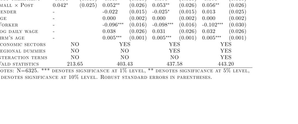
tics, (S3) controls for regional dummies, (S4) includes interaction terms. The coe¢cient of interest is the interaction term between the small …rm dummy and the post treatment dummy. The results are clustered around 4 and 8% and are statistically signi…cant in all but one case. More interestingly the sign is positive in all the speci…cations and for all the subsamples used for the estimations. This is somewhat reassuring, because it shows that there is a clear cut dominance of the enhancing e¤ect of EPL on CFL conversion into permanent jobs. The coe¢cients reported in table 7 con…rm the re-sults and can be interpreted as a robustness check. The estimates conducted on the subsample which limit the size of control …rms to the 50 employees threshold is of particular interest. Indeed, the increase in the comparabil-ity of treatment and control groups tends to emphasize the positive e¤ect of EPL on the job contract conversion rate. Moreover, even though a large number of observations are dropped, the magnitude of the e¤ect of the re-form is very similar to the one found in other speci…cations. In the baseline model the coe¢cient is 7%, and in all the other speci…cations is around 8% with a standard deviation of 0.03. This can be interpreted as evidence of a switching behavior of small …rms towards a more parsimonious use of work-ing and trainwork-ing contracts as a way to select workers. The threat of dismissal costs makes …rms more aware of the risk of separation, and CFL contracts represents a sort of insurance against this risk because …rms can acquire in-formation about workers, and - maybe more important - workers can …gure out how their working life will be if they decide to sign an open-ended con-tract in that …rm. Thus, …rms are more willing to select workers for their stable workforce among those already trained under CFLs and that are less likely to start a separation process. It should also be noted that since I adopt a regression control strategy, an important check is to look at the sensitivity of the estimates to the progressive inclusion of control variables22. From the
tables, it is straightforward to notice that the coe¢cients are substantially
stable after regional and sector dummies are included, as well as interaction terms are added to the regressions. For example, the …rst column of results in table 7 shows that the average treatment e¤ect ranges between 0:071 to
0:081. In particular, the e¤ect is equal to 0:071 in the baseline speci…cation, and once I progressively add workers’ and …rms’ characteristics plus economic sector dummies, regional dummies and interaction terms, the estimates are, respectively, 0:079, 0:081 and 0:080.
The results of this study have aslo policy implications. In the absence of EPL, a minor fraction of temporary workers is retained by …rms. This im-plies that …rms, anticipating this outcome, are less likely to improve training activities for …xed-term workers, reducing the overall degree of future work-ers employability. This channel acts through the slow productivity growth implied by less training activities.
5
Conclusions
Table 5: The e¤ect of the Italian 1990 reform on the job contract conversion rate
Regressors Linear probability model
(S1) (S2) (S3) (S4)
Small firms -0.199 (0.017) -0.157 (0.018) -0.156 (0.018) -0.155 (0.018)
Post treatment -0.053 (0.017) -0.066 (0.018) -0.066 (0.018) -0.066 (0.018)
Small Post 0.042 (0.025) 0.050 (0.025) 0.051 (0.025) 0.053 (0.025)
Gender - -0.021 (0.014) -0.023 (0.014) -0.013 (0.024)
Age - 0.000 (0.002) 0.000 (0.002) 0.000 (0.002)
Worker - -0.093 (0.015) -0.095 (0.015) -0.098 (0.029)
Log daily wage - 0.034 (0.025) 0.028 (0.025) 0.029 (0.025)
Firm’s age - 0.005 (0.001) 0.004 (0.001) 0.005 (0.001)
Economic sectors NO YES YES YES
Regional dummies NO NO YES YES
Interaction terms NO NO NO YES
Constant 0.596 (0.012) 0.370 (0.171) 0.348 (0.180) 0.327 (0.181)
F-statistics 74.18 33.56 17.16 15.27
Notes: N=6325. *** denotes significance at 1% level, ** denotes significance at 5% level, * denotes significance at 10% level. Robust standard errors in parentheses.
Table 6: Results from Probit estimations (full sample)
Regressors Probit estimates
(S1) (S2) (S3) (S4)
Small firms -0.199 (0.017) -0.161 (0.019) -0.161 (0.019) -0.160 (0.019)
Post treatment -0.054 (0.018) -0.069 (0.019) -0.070 (0.019) -0.070 (0.019)
Small Post 0.042 (0.025) 0.052 (0.026) 0.053 (0.026) 0.056 (0.026)
Gender - -0.022 (0.015) -0.025 (0.015) 0.013 (0.025)
Age - 0.000 (0.002) 0.000 (0.002) 0.000 (0.002)
Worker - -0.096 (0.016) -0.098 (0.016) -0.102 (0.030)
Log daily wage - 0.038 (0.026) 0.031 (0.026) 0.032 (0.026)
Firm’s age - 0.005 (0.001) 0.005 (0.001) 0.005 (0.001)
Economic sectors NO YES YES YES
Regional dummies NO NO YES YES
Interaction terms NO NO NO YES
Wald statistics 213.65 403.43 437.58 443.20
Notes: N=6325. *** denotes significance at 1% level, ** denotes significance at 5% level, * denotes significance at 10% level. Robust standard errors in parentheses.
Table 7: Estimation results from di¤erent subsamples
Subsamples
Model Description <50 PS1 PS2 PS3
(S1) Small firm -0.142 (0.022) -0.196 (0.017) -0.195 (0.017) -0.183 (0.018)
Post treatment -0.081 (0.026) -0.056 (0.018) -0.072 (0.018) -0.075 (0.019)
Small Post 0.071 (0.032) 0.047 (0.026) 0.059 (0.026) 0.057 (0.027)
(S2) Small firm -0.142 (0.023) -0.161 (0.019) -0.162 (0.019) -0.159 (0.019)
Post treatment -0.072 (0.028) -0.066 (0.020) -0.076 (0.020) -0.074 (0.021)
Small Post 0.079 (0.032) 0.053 (0.026) 0.063 (0.026) 0.059 (0.027)
(S3) Small firm -0.143 (0.023) -0.162 (0.019) -0.163 (0.019) -0.159 (0.020)
Post treatment -0.071 (0.028) -0.066 (0.020) -0.076 (0.020) -0.074 (0.021)
Small Post 0.081 (0.032) 0.055 (0.026) 0.064 (0.026) 0.060 (0.028)
(S4) Small firm -0.140 (0.023) -0.160 (0.019) -0.161 (0.019) -0.158 (0.020)
Post treatment -0.071 (0.028) -0.067 (0.020) -0.076 (0.020) -0.074 (0.021)
Small Post 0.080 (0.033) 0.057 (0.026) 0.066 (0.027) 0.063 (0.028)
N. obs 4493 6238 6035 5587
Notes: * denotes
References
Angrist, J. D. and Krueger, A.: 1999, Empirical Strategies in Labor Eco-nomics, Vol. 3A of Handbook of Labor Economics, Orley Ashenfelter and David Card edn, Elsevier Science, Amsterdam: North-Holland. Autor, D. H., Kerr, W. R. and Kugler, A. D.: 2007, Does Employment
Pro-tection Reduce Productivity? Evidence From US States,The Economic Journal 117, F189–F217.
Bassanini, A., Nunziata, L. and Venn, D.: 2008, Job Protection Legislation and Productivity Growth in OECD Countries, IZA Discussion Paper
(3555).
Blanchard, O. and Portugal, P.: 2001, What Hides behind an Unemployment Rate: Comparing Portuguese and U.S. Labor Markets, The American Economic Review 91(1), 187–207.
Boeri, T. and Jimeno, J.: 2005, The E¤ects of Employment Protec-tion: Learning from Variable Enforcement, European Economic Review
49(8), 2057–2077.
Cahuc, P. and Postel-Vinay, F.: 2002, Temporary Jobs, Employment Pro-tection and Labor Market Performance, Labour Economics 9, 63–91. Cahuc, P. and Zylberberg, A.: 2004, Labor Economics, The MIT Press. Contini, B., Cornaglia, F., Malpede, C. and Rettore, E.: 2002, Measuring
the impact of the Italian CFL programme on the job opportunities for the youths, laboratoriorevelli.it .
Eissa, N. and Liebman, J.: 1996, Labor Supply Response to the Earned Income Tax Credit, The Quarterly Journal of Economics 111(2), 605– 637.
Gagliarducci, S.: 2005, The Dynamics of Repeated Temporary Jobs, Labour Economics 12, 429–448.
Garibaldi, P.: 1998, Job Flow Dynamics and Firing Retrictions, European Economic Review 42, 245–275.
Garibaldi, P. and Pacelli, L.: 2008, Do Larger Severance Payments Increase Individual Job Duration?, Labour Economics 15, 31.
Ichino, A. and Riphahn, R.: 2005, The E¤ect of Employment Protection on Worker E¤ort: Absenteeism During and After Probation,Journal of the European Economic Association 3(1), 120–143.
Imbens, G. W. and Rubin, D. B.: 2008, Causal Inference, (forthcoming). Kugler, A. D. and Pica, G.: 2008, E¤ects of Employment Protection on
Worker and Job Flows: Evidence from the 1990 Italian Reform, Labour Economics 15(1), 78–95.
Lazear, E.: 1990, Job Security Provisions and Employment,Quarterly Jour-nal of Economics 105(3), 699–726.
Lee, M.-J.: 2005, Micro-Econometrics for Policy, Program, and Treatment E¤ects, Oxford University Press.
Lee, M.-J. and Kang, C.: 2006, Identi…cation for Di¤erence in Di¤erences with Cross-Section and Panel Data, Economics Letters 92(2), 270–276. Leonardi, M. and Pica, G.: 2007, Employment Protection Legislation and
Mortensen, D. and Pissarides, C.: 1994, Job Creation and Job Destruction in the Theory of Unemployment, Review of Economic Studies 61(3), 397– 415.
Rosenbaum, P. R. and Rubin, D. B.: 1983, The Central Role of the Propensity Score in Observational Studies for Causal E¤ects,Biometrika
70(1), 41–55.
Tattara, G. and Valentini, M.: 2005, Evaluating the Italian Training on the job Contract (CFL), Università Cà Foscari di Venezia.
Appendix
Subsamples
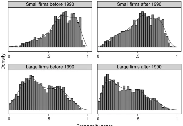
Since CFL workers can be observed in just one period, either before or after the 1990 reform, the data do not have a longitudinal component, but I am still able to build two waves. A crucial point is that these two waves must be comparable in order to proceed with the analysis. If the composition of small and large …rms varies substantially between waves, the empirical analysis becomes unfeasible. I check the plausibility of the strategy adopted to build the data by comparing the propensity score distributions for small and large …rms in both waves. Since the work of Rosenbaum and Rubin (1983), the propensity score has been widely used to reduce the dimension of the conditioning problem in matching methods. Since in this study, the set of covariates includes 35 variables, for whom I can only make inference on the marginal distributions, a practical solution is to look at the propensity score distributions.
wage and …rm’s age. Then, I run K KB logistic regressions including each
time a di¤erent covariate and I perform a likelihood ratio test for the addi-tional covariate. I use the LR-test statistics to rank the K KB covariates,
and among them I choose the one with the highest test statistic to enter the propensity score speci…cation. I repeat the procedure on the remaining covariates until none of the LR-test statistics is greater than the 2.71 cuto¤ value, which corresponds at a 10% level of signi…cance23. According to this
iterative procedure, I select a subset KS made up of eleven covariates. Using
the (KB +KS) set of covariates, I generate interaction terms24 and select
those who perform well in terms of likelihood ratio test, as before25. I then
estimate the propensity score according to the following logistic equation:
Pr (small …rm= 1) = 1
1 +e X (5)
where X contains all the selected covariates and the interaction terms. Figure 2 shows the estimated propensity score by …rm size, before and after the reform. The solid lines are kernel plots of the propensity score distribu-tions. From the inspection of the histograms, we can see that there are no drastic changes between the two waves of the cross-sections.
23The table with the LR-test statistics is available on request.
24Note that some of theN(N 1)=2possible interactions (whereN is the number of the
KB+KS covariates) are meaningless (interactions among regions and interactions among economic sectors), while other interaction terms have not been computed because of the small number of observations.
25I end up with …ve interactions, in particular the interaction of the worker variable
Figure 1: Propensity score distributions
0 .5 1
Small firms before 1990
0 .5 1
Large firms before 1990
0 .5 1
Small firms after 1990
0 .5 1
Large firms after 1990
De
nsi
ty
Propensity score