Inflation Volatility: An Asian Perspective

Munich Personal RePEc Archive

Inflation Volatility: An Asian Perspective

Rizvi, Syed Kumail Abbas and Naqvi, Bushra

Université Paris 1 Panthéon-Sorbonne

1 August 2009

Online at

https://mpra.ub.uni-muenchen.de/19547/

1

Inflation Volatility: An Asian Perspective

Syed Kumail Abbas Rizvi

_{Bushra Naqvi}

September 14, 2009

Abstract

The primary purpose of this study is to model and analyze inflation volatility in ten

selected Asian economies. We used quarterly data of inflation from 1987Q1 to 2008Q4

to model inflation volatility as time varying process through different symmetric and

asymmetric GARCH specifications. We also proposed to model inflation volatility on the

basis of cyclic component of inflation obtained from HP filter instead of actual inflation

when the latter does not fulfill the criterion of stationarity. Through news impact curves

we tried to highlight the behavior of inflation volatility in response to lagged inflation

shocks under different GARCH specifications for selected economies. Bivariate granger

causality test is also applied to analyze the direction of causality between inflation and

different volatility estimates.

We get few important results. At first, leverage parameter shows expected sign and is

significant for almost all countries suggesting strong asymmetry in inflation volatility.

The hyperbolic sign integral shape of news impact curves based on GJR-GARCH is

consistent with the results of our previous study based on Pakistani data (Rizvi and

Naqvi, 2008) and highlights the importance of inflation stabilization programs

particularly because of the subsequent evidences obtained in favor of bidirectional

causality running between inflation and inflation volatility. There are also evidences in

favor of the argument that cyclic component of inflation could be a used as a suitable

proxy of inflation for volatility estimation.

Keywords: Inflation Volatility, Uncertainty, GJR-GARCH, EGARCH, Asymmetry, Asia

JEL Classification: C22, E31, E37

2

1. Introduction

The primary purpose of this paper is to investigate about and to analyze the behavior of

inflation volatility in different Asian economies. There is a consensus about the negative

consequences of inflation volatility on different financial and economic variables which

eventually deteriorate the economic growth and welfare. Abundant literature has been

available on different channels through which inflation volatility distorts the decision

making regarding future saving and investment, the efficiency of resource allocation and

the level of real output. (Fischer 1981, Golob 1993, Holland 1993b)

However there are two issues which are still debatable and there exist significantly

different thoughts about them in economic literature. First issue is about the causality

running between inflation and inflation volatility. Friedman (1977), Ball and Cecchetti

(1990), Cukierman and Wachtel (1979), Evans (1991), and Grier and Perry (1998),

among others, provide evidences in support of a positive impact of average rate of

inflation on inflation volatility, which is more commonly known as “Friedman-Ball

Hypothesis”. On the other hand Cukierman-Meltzer (1986), Holland (1995), Baillie et al

(1996) for UK, Argentina, Brazil and Israel and Grier and Perry (1998) for Japan and

France provide some evidences, contrary to above and in support of causality running

from inflation volatility to inflation, which is more commonly known as

“Cukierman-Meltzer Hypothesis”.

Second issue is about the suitable proxy for inflation volatility or uncertainty. Most

common way to estimate inflation volatility is from surveys of expectations, such as

Livingston survey in the United States in which inflation volatility is captured as

variance of inflation forecasts across cross sectional data. However, in his remarkable

contribution, Engle (1983) first modeled inflation volatility as autoregressive or time

varying conditional hetersoscedasticity (ARCH), in which he used conventional inflation

3 (forecast errors) to vary overtime, suggesting that this variance could be used as a proxy

for inflation volatility. Empirical research on ARCH model often identified long lag

processes for the squared residuals, showing persistent effects of shocks on inflation

volatility. To model this persistence many researchers subsequently suggested

variations or extensions to the simple ARCH model to test the inflation uncertainty

hypothesis. Bollerslev (1986) and Taylor (1986) independently developed the

generalized ARCH (GARCH) model, in which the conditional variance is a function of

lagged values of forecast errors and the conditional variance. Beside Bollerslev (1986)

there are several studies which modeled inflation volatility through GARCH frameworks,

such as Bruner and Hess (1993) for US CPI data, Joyce (1995) for UK retail prices, Della

Mea and Peña (1996) for Uruguay, Corporal and McKiernan (1997) for the annualized

US inflation rate, Grier and Perry (1998) for G7 countries, Grier and Grier (1998) for

Mexican Inflation, Magendzo (1998) for Inflation in Chile, Fountas et al (2000) for G7

countries , and Kontonikas (2004) for UK. All these studies modeled inflation volatility

through GARCH model in one way or other.

The major drawback of typical ARCH or GARCH models is that they assume symmetric

response of conditional variance (volatility) to positive and negative shocks. However, it

has been argued that the behavior of inflation volatility is asymmetric rather than

symmetric. Brunner and Hess (1993), Joyce (1995), Fountas et al (2006), Bordes et al

(2007) are of the view that positive inflation shocks increases inflation volatility more

than the negative inflation shocks of equal magnitude. Beyond that there are some

evidences from Pakistani data that not only having lesser impact on inflation volatility,

negative inflation shocks can even contribute in reducing inflation volatility, Rizvi and

Naqvi(2008). If this is correct, the symmetric ARCH and GARCH models may provide

misleading estimates of inflation uncertainty [Crawford and Kasumovich, 1996].

The three most commonly used GARCH formulations to capture asymmetric behavior of

4 Jagannathan and Runkle (1993) and Zakoïan (1994), the Asymmetric GARCH (AGARCH)

model of Engle and Ng (1993), and the Exponential GARCH (EGARCH) model of Nelson

(1991).

In this paper we tried to model inflation volatility for ten South Asian economies with

the help of dynamic structure for mean inflation and different GARCH specifications for

inflation volatility. For those countries where inflation series is found to be non

stationary, we model cyclic component of inflation obtained through Hodrick Prescott

filter, in addition to actual inflation series to extract inflation volatility from it. We also

graphically depict the impact of inflation shock on degree of asymmetry of next period

volatility through News Impact Curves proposed by Pagan and Schwart (199). And

finally we present the categorized results of bivariate Granger Causality test between

inflation and different volatility estimates for the economies under consideration.

The paper is organized as follows: description of data and preliminary stationarity

analysis of time series is provided in section 2; section 3 presents the empirical

5

2. Description and Preliminary Analysis of Data

2.1 Core vs. Headline Inflation

The choice between core vs. headline inflation as a suitable proxy of inflation is crucial

while modeling inflation volatility. It is generally believed that headline inflation is more

volatile than core inflation due to the large commodity representation including oil and

food. Mishkin (2007) is of the view that despite of the fact that core inflation may not

represent a true picture of the inflation, monetary authorities should respond and target

core inflation as it is more appropriate than responding headline inflation due to its

inherently highly volatile and less persistent structure.

The above argument has certain shortcomings; many economists raised the questions

that if the core inflation does not truly represent the inflation in economy, do we really

need to follow or even control it? The second argument is the persistent increase in oil

prices during recent decades, which is definitely reflecting a changing global demand

structure for oil and thus the control of which is undoubtedly the part of the medium

term and the long term policies of monetary authorities.

The myth about core inflation as a better predictor of persistent inflation and thus

should be the key measure to watch, came under serious threat after the release of a

research conducted by Federal Reserve Bank of Philadelphia in May 2008 saying that

“We find that food and energy prices are not the most volatile components of

inflation and that, depending on which inflation measure is used, core inflation is

not necessarily the best predictor of total inflation”** _{. They also strongly suggest}

considering both core and headline inflation as opposed to only core inflation because

both measures provide independent information and the dual focus can significantly

improve the accuracy of inflation forecasting model.

**_{WORKING PAPER NO. 08-9 “CORE MEASURES OF INFLATION AS PREDICTORS OF TOTAL INFLATION” Theodore M. Crone, Swarthmore} College N. Neil K. Khettry, Murray, Devine & Company Loretta J. Mester, Federal Reserve Bank of Philadelphia and the Wharton School, University of Pennsylvania Jason A. Novak, Federal Reserve Bank of Philadelphia May 2008

6 In the light of above arguments and keeping in view the fact that our data set is

primarily composed of emerging or less developed countries where the oil price is the

major determinant of other products’ prices, the overall prices are downward sticky and

the percentage of disposable personal income on food consumption is more than 50

percent as opposed to developed countries where this percentage is between 9 to 15

percent, it is very difficult for monetary authorities to ignore oil and food prices while

modeling and coping with inflation. Therefore, we decide to model inflation volatility on

the basis of quarterly series of CPI calculated on Y-o-Y basis.

2.2 Data Set

Our data set is composed of quarterly estimates of inflation for 10 Asian economies;

China, Hong Kong, India, , Indonesia, Malaysia, Pakistan, Philippines, Singapore, South

Korea and Thailand. All data is taken from International Financial Statistics Database

(IFS) of IMF and covers the time period from 1987Q1 to 2008Q4.

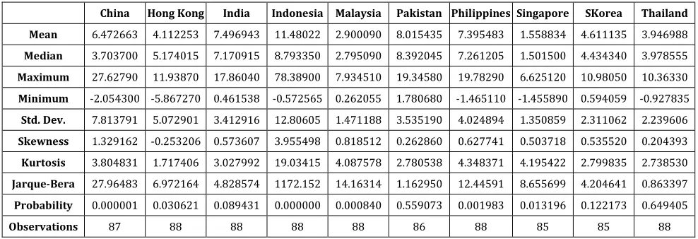
Table 1: Descriptive Statistics of Inflation in South Asian Economies (1987 to 2008)

China Hong Kong India Indonesia Malaysia Pakistan Philippines Singapore SKorea Thailand

Mean 6.472663 4.112253 7.496943 11.48022 2.900090 8.015435 7.395483 1.558834 4.611135 3.946988 Median 3.703700 5.174015 7.170915 8.793350 2.795090 8.392045 7.261205 1.501500 4.434340 3.978555 Maximum 27.62790 11.93870 17.86040 78.38900 7.934510 19.34580 19.78290 6.625120 10.98050 10.36330 Minimum -2.054300 -5.867270 0.461538 -0.572565 0.262055 1.780680 -1.465110 -1.455890 0.594059 -0.927835 Std. Dev. 7.813791 5.072901 3.412916 12.80605 1.471188 3.535190 4.024894 1.350859 2.311062 2.239606 Skewness 1.329162 -0.253206 0.573607 3.955498 0.818512 0.262860 0.627741 0.503718 0.535520 0.204393 Kurtosis 3.804831 1.717406 3.027992 19.03415 4.087578 2.780538 4.348371 4.195422 2.799835 2.738530 Jarque-Bera 27.96483 6.972164 4.828574 1172.152 14.16314 1.162950 12.44591 8.655699 4.204641 0.863397 Probability 0.000001 0.030621 0.089431 0.000000 0.000840 0.559073 0.001983 0.013196 0.122173 0.649405

Observations 87 88 88 88 88 86 88 85 85 88

2.3 Stationarity of Variables

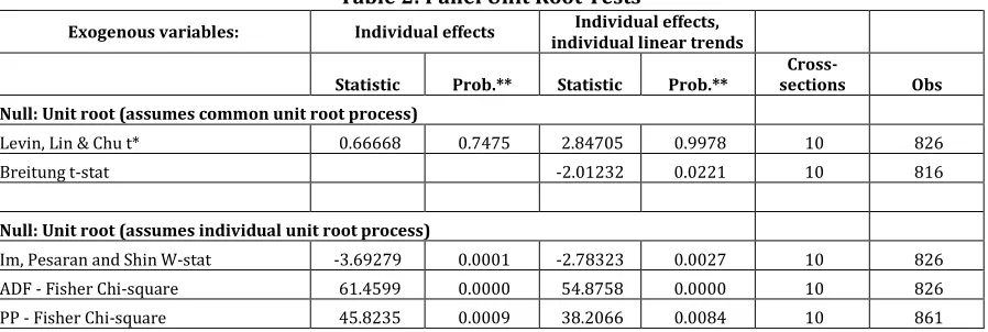
To check the order of integration, we conduct the panel unit root tests for inflation in

this section. Table 2 reports the summary statistics of five different panel unit root tests

each with two classifications, first with constant term only and the second with both

7 cross sections where as the rest of three assume individual unit root processes for each

cross section, which is more realistic assumption. Only LLC test does not reject the null

hypothesis of common unit root in both specifications, rest of the tests clearly reject the

null hypothesis of common or individual unit root and are highly significant.

Table 2: Panel Unit Root Tests

Exogenous variables: Individual effects Individual effects, individual linear trends

Statistic Prob.** Statistic Prob.**

Cross-sections Obs

Null: Unit root (assumes common unit root process)

Levin, Lin & Chu t* 0.66668 0.7475 2.84705 0.9978 10 826

Breitung t-stat -2.01232 0.0221 10 816

Null: Unit root (assumes individual unit root process)

Im, Pesaran and Shin W-stat -3.69279 0.0001 -2.78323 0.0027 10 826 ADF - Fisher Chi-square 61.4599 0.0000 54.8758 0.0000 10 826 PP - Fisher Chi-square 45.8235 0.0009 38.2066 0.0084 10 861

The rejection of null in IPS, ADF and PP test is little big vague in the sense that it leads us

to accept the alternative of “some cross sections without unit root”. To have a deep

insight about each cross section we report the Im, Pesaran and Shin W-statistics for

individual cross sections in table 3, considering only intercept term and automatic lag

selection based on SIC. The reason for dropping linear trend term is that in our opinion

economic theory does not provide enough evidences in support of assumption about the

presence of any long term linear trend in inflation rate.

Table 3: Unit Root Test Statistics for Individual Cross Section Cross section t-Stat E(t) E(Var) Lag Max Lag Obs

China -2.7397 -1.477 0.802 5 11 81 Hong Kong* -0.9262 -1.481 0.788 4 11 83 India* -1.4050 -1.427 0.855 8 11 79 Indonesia -6.4052 -1.526 0.749 1 11 86 Malaysia -2.7681 -1.526 0.749 1 11 86 Pakistan* -0.9892 -1.476 0.803 5 11 80 Philippines -2.4992 -1.478 0.801 5 11 82 Singapore -2.0354 -1.525 0.750 1 11 83 SKorea -1.6866 -1.478 0.791 4 11 80 Thailand -3.8036 -1.526 0.749 1 11 86

8 From table 3 it is clear that at least in three countries which are Hong Kong, India and

Pakistan, t-statistic falls within the acceptance region of null of unit root, thus indicating

that inflation is non stationary there. Some other tests force us to believe the same thing

for Singapore and South Korea.

3. Empirical Framework

3.1 Construction of Mean Equation

There are certain economic and financial variables believed as important determinants

of inflation however we choose to model inflation dynamically, through an

autoregressive process (equation 1) in which inflation in one period is a function of its

lagged values. The reason for the inclusion of autoregressive term is straight

forward as Inflation, like many other economic variables, has shown strong inertia in

various studies. Cecchetti et al (2000), for US data, verified that none of the single

indicator out of 19 which are generally believed as an important determinant of

inflation, is able to improve the forecasts of autoregressive model clearly and

consistently. Binner et al (2009) also did not find significant support for the usefulness

of monetary aggregates in the process of forecasting inflation thus declared non linear

autoregressive model based on kernel methods as the best for the job.

The decision about the number of lags to be included in each cross section is based on

AIC and BIC. To check the presence of serial correlation in the residuals of AR model we

applied Breusch-Godfrey test and Ljung-Box Q statistics and then introduced

appropriate AR or MA terms for errors, as indicated by the correlogram, to eliminate

serial correlation (equation 2). There are many approaches to estimate models with AR

or MA error specifications like Cochrane-Orcutt, Paris-Winsten, Hatanaka, and

Hildreth-Lu procedures but they all are bound to operate in the horizon of standard linear

regression thus there results are not reliable when model contains lagged dependent

9 (1993, p. 329-341), Greene (1997, p. 600-607)]. To overcome this problem we applied

non linear estimation which is applicable even when model contain endogenous right

hand side variables and whose estimates are asymptotically equivalent to maximum

likely hood estimates and are asymptotically efficient. Fair (1984, p. 210-214), Davidson

and MacKinnon (1993, p. 331-341).

∑ Equation 1

∑ ∑ Equation 2

3.2 Modeling of Non stationary Inflation:

One can argue that the results obtained from the above model could possibly be

questionable for those countries where inflation series is found to be non-stationary. To

cope with this problem we proposed to model cyclical component of inflation, obtained

from Hodrick-Prescott filter, instead of Inflation to capture conditional variance or

inflation volatility through different GARCH specifications. The use of HP filter as a tool

for detrending is popular among researchers and its advantage, compared to traditional

differencing method, is that it removes only the slowly moving stochastic long term

trend from the original series thus keeping the persistence of data preserved in the

cyclic component. There are also evidences that first difference detrending removes not

only the trend but also some other useful information from the original series (Fiorito,

2008). Though there are certain limitations of HP filter pointed out by Harvey and

Jaeger (1993) such as spurious cyclical structure and spurious correlations when the

series is I(0), but still its usability in detrending cannot be ruled out

completely,(Ahumada, 1999). Thus keeping in view the above methodology we model

(Cyclic component of Inflation) as well as (Inflation) for Hongkong, India, Pakistan,

Singapore and South Korea where we don’t have enough evidences to reject the null of

unit root in Inflation series. Structure of equation 1 will become as equation 3 and rest of

10

∑ Equation 3

3.3 Volatility Estimates:

We choose GARCH specification to model inflation volatility as there are many evidences

available which suggest that GARCH specification is better than ARCH. In an study about

the performance of different volatility models, (Hansen and Lunde, 2001) find that while

comparing the competing models on the basis of their out of sample predictive abilities,

they do not have enough evidences to reject the hypothesis that none of other volatility

models are better than GARCH (1,1).

∑ ∑ Equation 4

Where ! 0, $ % &'( , , … … . ,

$ % &'( , , … … . ,

GARCH is more parsimonious compared to ARCH as it captures the effect of infinite

number of past squared residuals on current volatility with only three parameters and is

less likely to breach non-negativity constraints artificially imposed on ARCH, Bollerslev

(1986). But the primary restriction of GARCH model is that it enforces a symmetric

response of volatility to positive and negative shocks. According to Brunner and Hess

(1993) and Joyce (1995), a positive inflation shock is more likely to increase Inflation

volatility via monetary policy mechanism, as compared to negative inflation shock of

equal size. If it is true then we cannot rely on the estimates of symmetric ARCH and

GARCH models and will have to go for asymmetric GARCH models. To capture those

asymmetric responses of inflation volatility we used two asymmetric formulations of

GARCH which are GJR or Threshold GARCH (TGARCH) models of Glosten, Jagannathan

and Runkle (1993) and Zakoïan (1994), and the exponential GARCH (EGARCH) model

11 GJR-GARCH is simply an extension of GARCH(p,q) with an additional term to capture the

possible asymmetries (leverage effects). The conditional variance is now

+ , Equation 5

Where - _.= 1, if / _. < 0, otherwise - _.= 0. If the asymmetry parameter 0 is negative

then negative inflationary shocks result in the reduction of inflation volatility. (Bordes et

al. 2007).

Conditional volatility is positive when 1 ! 0, 2₃ $ 0, 2₃ 0₃ /2 $ 0 for 6 1 89 :, and

;< $ 0, for = 1 89 >. The process is covariance stationary if and only if ?∑@3 . 23 03A/

2 ∑B< .;< C 1D(Hentschel 1995)

The exponential GARCH model was proposed by Nelson (1991). There are various ways

to express the conditional variance equation, but one possible specification is

EFG ∑ EFG ∑ H I

J IH ∑ +

K I

J I Equation 6

Both of these asymmetric GARCH models have several advantages over the traditional

ARCH and GARCH specifications. First, variance specification represented in equations 5

and 6 make it possible to capture the asymmetric effects of good news and bad news on

one period ahead conditional variance, which is preferable in the context of modeling

Inflation and Inflation volatility. Additionally in EGARCH specification, since the

conditional variance is modeled in its logarithmic form, then even in the presence of

negative parameters, L will be positive thus relieving the non-negativity constraints

artificially imposed on GARCH parameters.

3.4 Impact of News on Volatility (Policy Effectiveness)

For further investigation of asymmetric behavior of inflation volatility, we analyzed the

effects of news on volatility or inflation uncertainty with the help of “News Impact

Curve”. The idea was primarily proposed by Pagan and Schwert (1990) and Engle and

12 information at t-2 and earlier, we can examine the implied relation between / _. and L

which we called as “News Impact Curve”. Primary purpose of News Impact Curve is to

graphically represent the impact of past shocks of inflation (news) on current volatility.

It is a pictorial representation of the degree of asymmetry of volatility to positive and

negative shocks and it plots next period volatility L that would arise from various

positive and negative values (news) of past inflation shocks (/ _.) [Pagan and Schwert,

1990], which will effectively help in determining the effectiveness of inflation

stabilization programs and inflation targeting policies. For the standard GARCH model,

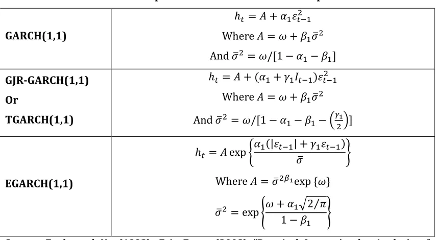
news impact curve is a quadratic function centered at / _. 0. The equations of news

impact curve for the GARCH, GJR-GARCH and EGARCH models are provided in table 4.

Table 4: News Impact Curve for different GARCH processes

GARCH(1,1)

L M 2./N .

Where M 1 ;_.OPN

And OPN 1/Q1 R 2_.R ;_.D

GJR-GARCH(1,1)

Or

TGARCH(1,1)

L M 2. 0.- . /N .

Where M 1 ;_.OPN

And OPN 1/Q1 R 2_.R ;_.R ST_NUVD

EGARCH(1,1)

L M exp Z2. |/ .| 0_OP ./ . \

Where M OPN]Uexp ^1_

OPN _{exp `}1 2.J2⁄

1 R ;. b

Source: Engle and Ng (1993), Eric Zevot (2008) “Practical Issues in the Analysis of Univariate GARCH Models”

Where L is the conditional variance at time t, / _.is inflation shock at time t-1, OP is the

unconditional standard deviation of inflation shocks, 1 and ;_. are constant term and

parameter corresponding to L _.in GARHC, GJR-GARCH and EGARCH specifications.

The shape of news impact curve depends upon the slope values for positive and negative

shocks. For GARCH specifications slope values are same for all shocks thus generating

13

/ .! 0, the slope of NIC is equal to 2_.only and equals to 2_. 0_. when / _.C

0 which is a case of good news where 0_.is asymmetry parameter or leverage parameter

in GJR-GARCH and EGARCH specifications.

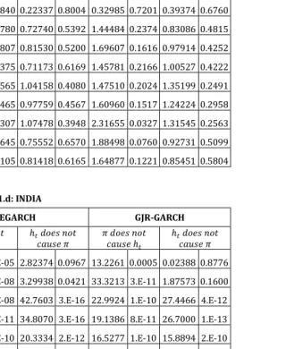
3.5 Direction of Causality between Inflation and Inflation Volatility

(Granger Causality Test)

In order to investigate the direction of causality running between Inflation and Inflation

volatility and to check the authentication of Friedman-Ball or Cukierman-Meltzer

hypotheses, we implement Bivariate Granger-Causality test up to 10 lags, between

inflation and volatility estimates obtained from GARCH, EGARCH and GJR-GARCH

specifications. We report Wald statistics and corresponding p-values for the null

hypothesis that “X does not cause Volatility” in the first column and that “Volatility does

not cause X” in the second column by placing Inflation as X for all countries and by

placing cyclic component of Inflation as X for those countries where inflation is

nonstationary under GARCH, EGARCH and GJR-GARCH specifications (Appx. Table 11.a

to 11.o).

4. Results and Findings

4.1 GARCH Specification

We checked the stability condition of GARCH specification for all countries and found

some violations, such as in case of South Korean inflation and its cyclic component the

ARCH coefficient 2 is negative, for Malaysia and Indonesia the GARCH coefficient ; is

negative; in addition to that there is also a violation of second order stationarity

condition in case of China and Indonesia where 2 ; ! 1 due to which, for these two

countries, the long run mean reverting level of volatility is negative. (Appx. Table 5)

4.2 GJR-GARCH Specification

The results of GJR GARCH are very promising. Almost for all instances, except for the

14 negative (significant at 5 percent or below for Pakistan, China, Indonesia, Thailand and

India) which is expected and indicating the fact that negative inflation shocks (good

news) in one period reduce the next period volatility. The condition for volatility to be

covariance stationary i.e.; ?∑@_{3 .} 2₃ 0₃A/2 ∑B_{< .};_<C 1D is also fulfilled for all cases.

However the non negativity constraint Q 2₃ 0₃ /2 $ 0] is not fulfilled in case of

Pakistan, Indonesia, Thailand and India, the obvious reason for which is that the

asymmetry parameter is much larger as well as highly significant than ARCH coefficient

for these countries 0₃ ! 2₃ . (Appx. Table 5)

4.3 EGARCH Specification

EGARCH specification provides us the relationship between lagged shocks of Inflation

and the logarithm of the conditional volatility. Because of this logarithmic specification,

EGARCH is convenient to handle compared to other GARCH specifications as there are

no restrictions on its parameters. In EGARCH specification, past negative shocks have an

impact 2₃R 0₃ on the log of the conditional variance, while it is 2₃ 0₃ for positive

shocks. Generally it is observed that impact is greater in case of negative shocks

Q 23R 03 ! 23 03 D because 03 is expected to be negative or less than zero, but that

assumption is valid only if we are modeling returns. For Inflation, the converse is true;

here we must expect that 0₃ is positive so that Q 2₃R 0₃ C 2₃ 0₃ D and the impact is

lesser on conditional volatility in case of negative inflation shocks (good news)

compared to the situation of positive inflation shocks (bad news), [reported in the last

two columns of Appx. Table 5]. In can also be viewed in Appx. Table 8, that asymmetry

parameter 0₃ is positive as per expectation in all 15 instances and is significant at 5

percent or below in 8 out of 15 instances.

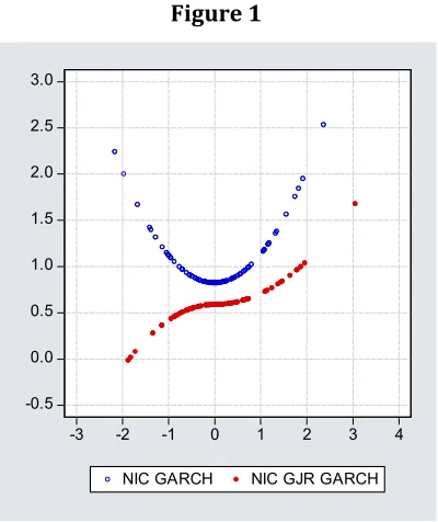
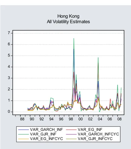
4.4 News Impact Curves

News impact curves obtained by using the equations of Table 4 are reported in Appx.

15 and Thailand where the news impact curve based on GJR GARCH is quite different from

its widely believed parabolic shape as mentioned below in figure 1.

Figure 1

This hyperbolic sign integral shape of GJR-NIC is extremely important for monetary

authorities and highlights the importance of inflation stabilization programs or inflation

targeting policies, which reduces the next period volatility (Jonhson, 2002). The results

are also consistent with our previous study (Rizvi and Naqvi, 2008) where the same

hyperbolic sign integral shape of GJR-NIC was found for Pakistani inflation with a data

set consists of relatively larger time period.

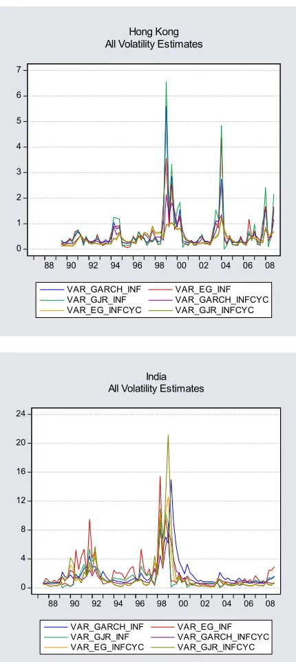
4.5 Modelling cyclic component of Inflation to capture Inflation Volatility

As we mentioned above that for the countries where we found inflation nonstationary

we ran additional regressions of cyclic component of inflation and modelled inflation

volatility based on the residuals of cyclic inflation. We then compare the volatility based

on inflation and the volatility based on cyclic component of inflation for these countries

to check how much reliable this procedure is in the volatility estimation when the

original series is nonstationary. Appx. Table 9 reports the results of tests of equality of

mean and variance between the two volatility estimates based on Inflation and on its

16 presented below in Figure 2, for other four countries it is provided in Appx. Figure 2.a to

2.e) T-test and Anova F-test assume the equal mean and variance for both volatility

estimates where as Satterthwaite-Welch t-test and Welch F-test assume equal mean but

allow for unequal variances. According to these results we can not reject the null of

equal mean and variance of both volatility estimates in four out of five countries under

GJR-GARCH specification. Put it in another way, it doesn’t matter whether we model

inflation volatility from total inflation or its cyclic component because there are

evidences that the volatility estimates obtained from both variables are close enough as

long as we applied GJR-GARCH specification.

Figure 2

4.6 Causality between Inflation and Inflation Volatility

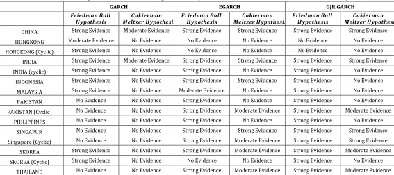
Appx. Table 10 reports the categorized results based on the quantitative results

provided in Appx. Table (11.a to 11.o) and highlights the fact that GARCH specification is

not very successful in capturing the causality running between inflation and inflation

volatility. Though the results are cumbersome but if we focus on asymmetric models

(EGARCH and GJR-GARCH) the results strongly favor the presence of Friedman-ball

17 hypothesis and clearly reject the presence of Cuckierman-meltzer hypothesis for

Indonesia, Malaysia, Pakistan and Phillipines. The results for other countries are though

biased in favour of Friedman ball hypothesis but are mixed and support significantly the

presence of both hypothesis, leading us to the conclusion that there is a bidirectional

causality running between inflation and inflation volatility. Hongkong is a special case

for which both asymmetric models strongly reject the presence of any causality between

inflation and volatility no matter whether we base our analysis on total inflation or on

the cyclic component of inflation.

5. Conclusion

This study contributes the following in the existing body of knowledge. First of all it can

be argued that the asymmetric GJR-GARCH and EGARCH models performed better than

symmetric GARCH in capturing inflation volatility for selected Asian economies. The

hyperbolic sign integral shape of news impact curve based on GJR-GARCH for India,

Indonesia, Pakistan and Thailand is not only consistent with the results of our previous

study based on Pakistani data (Rizvi and Naqvi, 2008) but also highlight the importance

of inflation stabilization programs and inflation targeting policies where negative

inflation shocks reduces one period ahead volatility which will subsequently reduces

inflation in further periods and so on. Evidences of bidirectional causality between

inflation and inflation volatility also strengthen the idea of having such type of chain

reaction. It can also be claimed that volatility estimates obtained from total inflation and

cyclic component of inflation exhibit the equal mean and variance properties under

GJR-GARCH specification, thus making the cyclic component of inflation, obtained from HP

filter, a suitable proxy of inflation in volatility modelling for those countries where

18

References

Ahumada, H., Garegnani, M. L. (1999), “Hodrick-Prescott Filter in Practice”, Economica-(National-University-of-La-Plata); 45(4), pages 61-76.

Andersen, T.G., Bollerslev, T. (2006), "Volatility and Correlation Forecasting", Handbook of Economic Forecasting, Vol. 1.

Apergis, N. (2006), “Inflation, output growth, volatility and causality: evidence from panel data and G7 countries”, Economics Letters, 83 (2004) 185-191.

Ball, L. (1992), “How does inflation raise inflation uncertainty?”, Journal of Monetary

Economics, 29, 371‐388.

Berument, H. et al (2001), “Modeling Inflation Uncertainty Using EGARCH: An Application to Turkey”, Bilkent University Discussion Paper.

Bilquees, F. (1988), “Inflation in Pakistan: Empirical Evidence on the Monetarist and Structuralist Hypotheses”, The Pakistan Development Review 27:2, 109–130.

Binner, J. M. et al (2009), “Does Money Matter in Inflation Forecasting?”, Federal Reserve

Bank of St. Louis, Working Paper Series, 2009-030A.

Bollerslev, T. (1986), “Generalized Autoregressive Conditional Heteroscedasticity”,

Journal of Econometrics, 31, 307‐27.

Bollerslev, T., and J.M. Wooldridge, (1992), “Quasi-Maximum Likelihood Estimation and Inference in Dynamic Models with Time-Varying Covariances”, Econometric Reviews, 11,

143-172.

Bokil, M. and Schimmelpfennig, A. (2005), “Three Attempts at Inflation Forecasting in Pakistan”, IMF Working Paper, WP/05/105.

Bordes, C. et al (2007), “Money and Uncertainty in the Philippines: A Friedmanite perspective”, Conference paper, Asia-Link Program.

Bordes, C. and Maveyraud, S. (2008), “The Friedman’s and Mishkin’s Hypotheses (re)considered”, Unpublished.

Brunner, A.D. and Hess, G.D. (1993), “Are Higher Levels of Inflation Less Predictable? A State-Dependent Conditional Heteroscedasticity Approach”, Journal of Business &

Economic Statistics, Vol. 11, No. 2, (Apr., 1993), pp. 187-197.

Brunner, A.D. and Simon, D.P. (1996), “Excess Returns and Risk at the long End of The Treasury Market: an EGARCH-M Approach”, The Journal of Financial Research, 14, 1,

443-457.

Caporale, T and McKiernan, B. (1997), “High and Variable Inflation: Further Evidence on the Friedman Hypothesis”, Economic Letters 54, 65-68.

19 Chaudhary, M. Aslam, and Naved Ahmad, (1996), “Sources and Impacts of Inflation in Pakistan,” Pakistan Economic and Social Review, Vol. 34, No. 1, pp. 21–39.

Cosimano, T. and Dennis, J. (1988), “Estimation of the Variance of US Inflation Based upon the ARCH Model”, Journal of Money, Credit, and Banking, 20(3) 409-423.

Crowford, A. and Kasumovich, M. (1996), “Does Inflation Uncertainty vary with the Level of Inflation?”, Bank of Canada, Ottawa Ontario Canada K1A 0G9.

Engle, R. (1982), “Autoregressive Conditional Heteroscedasticity with Estimates of United Kingdom Inflation”, Econometrica, 987-1007.

Fiorito, R. (2008), “Growth and Business Cycle Components”, Revised draft.

Fountas, S. et al (2000), “A GARCH model of Inflation and Inflation Uncertainty with Simultaneous Feedback”.

Fountas, S. et al (2006), “Inflation Uncertainty, Output Growth Uncertainty and Macroeconomic Performance”, Oxford Bulletin of Economics and Statistics, 68, 3 (2006) 0305-9049.

Franses, P.H. (1990), “Testing For Seasonal Unit Roots in Monthly Data”, Econometric Institute Report, No.9032A, Erasmus University, Rotterdam.

Friedman, M. (1977), “Nobel Lecture: Inflation and Unemployment”, Journal of Political Economy, Vol. 85, 451-472.

Glosten, L. R., R. Jagannathan and D. Runkle, (1993), “On the Relations between the Expected Value and the Volatility of the Normal Excess Return on Stocks”, Journal of Finance, 48, 1779-1801.

Golob, John E. (1994), “Does inflation uncertainty increase with inflation?”, Federal Reserve Bank of Kansas City - Economic Review. Third Quarter 1994.

Grier,K., Perry, M. (2000), “The effects of real and nominal uncertainty on inflation and output growth: some GARCH-M evidence”, Journal of Applied Econometric 15, 45-48.

Guay, A., St-Amant, P. (2005), “Do the Hodrick-Prescott and Baxter-King Filters Provide a Good Approximation of Business Cycles?”, Annales d’économie et de Statistique– N° 77 –

2005.

Harvey, A., and Trimbur, T. (2008), “Trend Estimation and the Hodrick-Prescott Filter”,

J. Japan Statist. Soc. Vol. 38 No. 1, 41–49

Hafer, R. W. (1985), “Inflation Uncertainty and a test of the Friedman Hypothesis”,

Federal Reserve Bank of St. Louis Working Paper 1985-006A.

Holland, A. S. (1984), “Does Higher Inflation Lead to More Uncertain Inflation?”, Federal Reserve Bank of St. Louis Review 66, 15-26.

20 Johnson, C. A. (2002), “Inflation Uncertainty In Chile: Asymmetries and the News Impact Curve”, Revista de Análisis Económico Vol. 17, Nº 1, 3-20.

Khalid, A. M. (2005), “Economic Growth, Inflation and Monetary Policy in Pakistan: Preliminary Empirical Estimates”, The Pakistan Development Review,44 : 4 Part II (Winter 2005) pp. 961–974.

Khan, M. S., and S. A. Senhadji (2001), “Threshold Effects in the Relationship between Inflation and Growth”, IMF Staff Papers 48:1.

Khan, A. H., and M. A. Qasim (1996)’ “Inflation in Pakistan Revisited”, The Pakistan Development Review 35:4, 747–759.

Khan, M. S., and A. Schimmelpfennig (2006), “Inflation in Pakistan: Money or Wheat?”,

IMF Working Paper, wp/06/60.

Koutmos, G., and G.G. Booth, (1995), “Asymmetric Volatility Transmission in International Stock Markets”, Journal of International Money and Finance, 14, 747-762.

Lunde, A. and Hansen, P. R. (2005) “A forecast comparison of volatility models: does anything beat a GARCH(1,1)?”, Journal of Applied Econometrics, vol. 20(7), pages 873-889.

Malik, W. Shahid and Ahmad, A. Maqsood (2007), “The Taylor Rule and the Macroeconomic performance in Pakistan”, The Pakistan Development Review, 2007:34.

Malik, W. Shahid (2006), “Money, Output and Inflation: Evidence from Pakistan”, The Pakistan Development Review 46:4.

Nas, T. F. and M.J. Perry, (2000), “Inflation, Inflation Uncertainty and Monetary Policy in Turkey”, Contemporary Economic Policy, 18, 170-180.

Nelson, D.B. (1991), “Conditional Heteroscedasticity in Asset Returns: A New Approach”,

Econometrica, 59, 347-370.

Price, Simon, and Anjum Nasim, (1999), “Modeling Inflation and the Demand for Money in Pakistan: Cointegration and the Causal Structure,” Economic Modeling, Vol. 16, pp. 87– 103.

Thornton, J. (2006), “High and variable inflation: further evidence on the Fried- man hypothesis”, Southern African Journal of Economics, 74, 167-71.

Tse, Y., and G.G. Booth, (1996), “Common Volatility and Volatility Spillovers Between U.S. and Eurodollar Interest Rates: Evidence from The Features Market”, Journal of Economics and Business, 48, 299-312

Qayyum, A. (2006), “Money, Inflation and Growth in Pakistan”, The Pakistan Development Review 45 : 2 (Summer 2006) pp. 203–212.

Rizvi, S.K.A., and Naqvi, B., (2008), “Asymmetric Behavior of Inflation Uncertainty and Friedman-Ball Hypothesis: Evidence from Pakistan”, 26th _{Symposium on Money, Banking}

and Finance, Orleaons, France.

Zivot, E. (2008), “Practical Issues in the Analysis of Univariate GARCH Models”,

1 | A p p x

! "# $ %&' ('( ) * + &, #& ' ,-' (&,

Appendix -Figure 1

. /

$ %&' ('( ) * + &, #& ' ,-' (&,

/ / / .

! "# $ %&' ('( ) 0 + &, ) '( & &, , &- ,-' (&,

/ / /

1 $ %&' ('( ) 0 + &, ) '( & &, , &- ,-' (&,

.

.

2 !2 $ %&' ('( ) 0 + &, #& ' ,-' (&,

.

2 !2 $ %&' ('( ) 0 + &, ) '( & &, , &- ,-' (&,

!2 $ %&' ('( ) 0 + &, #& ' ,-' (&,

/ / /

1 $ %&' ('( ) 0 + &, #& ' ,-' (&,

.

3 4 5" $ %&' ('( ) 0 + &, #& ' ,-' (&,

/ / /

!2 $ %&' ('( ) 0 + &, ) '( & &, , &- ,-' (&,

/ / / / . . .

# 4 1$ %&' ('( ) 0 + &, #& ' ,-' (&,

. /

" 6 $ %&' ('( ) 0 + &, ) '( & &, , &- ,-' (&,

44 "$ %&' ('( ) 0 + &, #& ' ,-' (&,

/ / / / // / 7

" 6 $ %&' ('( ) 0 + &, #& ' ,-' (&,

/ 8 8/ 8

.

2 | A p p x

APPENDIX-Tables

Table 5: Coefficients Restrictions on Volatility Models

GARCH (Mean Reverting Level)

GARCH (Stability)

GJR-GARCH (Covariance Stationarity)

GJR –GARCH (Non Negativity)

EGARCH EGARCH CHINA -8.2851 1.020863 0.456016 0.098152 0.201157 0.843743 HONGKONG 0.817041 0.727299 0.395387 0.438464 1.247568 1.531182 HONGKONG (Cyclic) 0.937769 0.860247 0.657212 0.07826 0.366703 0.688071 INDIA 4.417416 0.946739 0.542511 -0.09041 -0.6009 0.908148 INDIA (cyclic) 1.610521 0.849445 0.625568 0.292448 0.820412 1.112438 INDONESIA -4.37187 1.854417 0.269814 -0.23007 -2.33769 0.30183

MALAYSIA 0.419635 0.101467 -0.08363 0.160531 0.924166 0.925238 PAKISTAN 2.066967 0.65295 0.564163 -0.07614 -0.40042 0.426501 PAKISTAN (Cyclic) 7.629162 0.970386 0.306752 -0.0505 -0.15674 0.830713 PHILIPPINES 5.358836 0.918545 0.15968 0.044748 0.144877 0.996703 SINGAPUR 0.249842 0.534586 0.148038 0.015517 0.099954 0.505912 Singapore (Cyclic) 0.346369 0.980668 0.810881 0.092052 -0.08109 0.074869 SKOREA 1.137714 0.533554 0.659215 0.410593 1.15812 1.172058 SKOREA (Cyclic) 0.871926 0.47909 0.548528 0.299523 0.709121 1.246789 THAILAND 1.179098 0.605412 0.831552 -0.0863 -0.28006 0.427316

*Bold Values represent violations

Table 6: GARCH Specification

Country CHN HKN1 _HKN(Cyc) 1 _{IND IND(Cyc) NDS MLY PAK PAK(Cyc) PHL SNG SNG(Cyc) SKOR SKOR(Cyc) TLN}

0.045954 0.018922 -0.001049 0.058756 -0.005063 1.484208*** 0.281897* 0.181303 -0.057884 0.134991 0.015423 -0.000792 -0.018147 -0.001391 0.097857 1.603851*** 1.535378*** 1.230251*** 1.249537*** 0.936348*** 1.093169*** 1.304491*** 1.484289*** 1.271754*** 1.500361*** 1.523460*** 1.073894*** 0.986233*** 0.753511*** 1.348317*** -0.635760*** -0.548384*** -0.384900** -0.263443 _{-0.258466 -0.308437*** -0.404359*** -0.511078*** -0.466799*** -0.526718*** -0.535463*** -0.318257**} -0.375148**

-0.522387*** -0.488810**

-0.365908*** -0.408268*** -0.266862*** -0.327085*** -0.624402*** -0.548687***

-0.640871*** -0.915237*** -0.960053*** -0.926633*** -0.873307*** -0.898275*** -0.959262*** -0.971121*** -0.759718*** 0.172852 0.222808*** 0.131056 0.235276 0.242472 3.735401*** 0.377056*** 0.717341 0.225930 0.436504* 0.116280 0.006696 0.530682*** 0.454195** 0.465258 0.419361* 0.670459** 0.446452 0.376525** 0.331923** 1.884675*** 0.546886* 0.355595** 0.432361** 0.385109** 0.008386 0.087615* -0.067087 -0.040918*** 0.304677 0.601502*** 0.056840 0.413795 0.570214*** 0.517522*** -0.030258 -0.445419 0.297355 0.538025*** 0.533436*** 0.526200 0.893053*** 0.600641*** 0.520008** 0.300735

Adj R2

0.962878 0.977696 0.773874 0.852128 0.776289 0.847551 0.769835 0.877253 0.705477 0.896286 0.884522 0.805243 0.892215 0.775941 0.804962

AIC 3.439067 2.149183 2.064715 3.241209 _2.834162 5.101463 1.867303 3.268057 3.091147 3.338663 1.363933 0.984167 2.626359 2.351225 2.756383

SIC 3.640226 2.390896 2.306428 3.440982 3.033935 5.306914 2.072755 3.476485 3.299574 3.538436 1.567932 1.188166 2.799988 2.524855 2.956156

F-Stat _{364.1335*** 483.1825*** 38.64545*** 82.63722*** 50.15907*** 76.05417*** 46.15348*** 95.09971*** 32.53841***} 123.4270 105.6825*** 57.50610*** 138.4101*** 58.48779*** 59.46863***

1_{For Hong kong and its cyclic component consider and as and respectively}

3 | A p p x

Table 7: GJR GARCH or TGARCH Specification

Country CHN HKN1 _HKN(Cyc) 1 _{IND IND(Cyc) NDS MLY PAK PAK(Cyc) PHL SNG SNG(Cyc) SKOR SKOR(Cyc) TLN}

0.075365 0.050665 0.003795 0.146628* -0.014457 1.754165*** 0.268897 0.219229 0.016632 0.148204 0.004074 0.004243 0.082058 -0.004631 -0.056919 1.538845*** 1.615259*** 1.202471*** 1.379822*** 0.711794*** 1.485867*** 1.188609*** 1.493402*** 1.222602*** 1.496904*** 1.398911*** 1.196454*** 0.964142*** 0.744053*** 1.274895*** -0.580911*** -0.629885*** -0.379042*** -0.403882*** -0.080039 -0.636588*** -0.281512* -0.517517*** -0.380957*** -0.526335*** -0.413944*** -0.521752*** -0.269251***

-0.525595*** -0.496227***

-0.384515*** -0.389596*** -0.426080*** -0.369747*** -0.603399*** -0.557872***

-0.576702*** -0.916417*** -0.943847*** -0.932085*** -0.904857*** -0.892173*** -0.970195*** -0.947597*** -0.892648*** 0.179292* 0.157279** 0.064695 0.292477*** 0.108094* 5.576977 0.264034*** 0.301625 0.382819** 0.683623*** 0.111098* 0.032199 0.090362* 0.078963** 0.062652* 1.154837*** 1.275976* 0.537534 0.526391** 0.845174 0.257231 0.988899** 0.394843** 1.031866** 1.305053* 0.622322* -0.141545*** 0.976033*** 1.189094*** 0.116599 -0.958532** -0.399049 -0.381014 -0.707217*** -0.260279 -0.717372** -0.667837 -0.547115*** -1.132863*** -1.215558 -0.591289 0.325648 -0.154847 -0.590048 -0.289203** 0.357863*** -0.043077 0.578952** 0.632924*** 0.333120 0.499884 -0.244165 0.640299*** 0.357250 0.114932 0.132521 0.718829*** 0.248622*** 0.249005** 0.917854***

Adj R2 _{0.959473 0.977339 0.769251 0.844983 0.759167 0.905427 0.767075 0.877706 0.696557 0.893621 0.877090 0.811574 0.890053 0.770677 0.799030} AIC 3.335648 2.100246 2.056323 3.066536 2.736736 5.200215 1.867619 3.114269 2.955616 3.297456 1.249534 0.871409 2.132409 1.895128 2.626257

SIC 3.565545 2.372174 2.328251 3.294847 2.965047 5.435017 2.102421 3.352472 3.193818 3.525768 1.482675 1.104550 2.334977 2.097696 2.854568

F-Stat _{285.0969*** 416.1121*** 33.08692*** 67.18970*** 39.27740*** 111.7826*** 39.10741*** 81.99744*** 26.90655*** 103.0048*** 84.59353*** 51.45484*** 112.9851*** 47.48904*** 49.27834***}

Table 8: EGARCH Specification

Country CHN HKN1 _HKN(Cyc) 1 _{IND IND(Cyc) NDS MLY PAK PAK(Cyc) PHL SNG SNG(Cyc) SKOR SKOR(Cyc) TLN}

0.083643 0.041972 0.009608 0.116437 -0.012479 1.849843*** 0.282653** 0.115142 0.029709 0.148201 0.004435 -0.003575 0.071171 0.000822 0.010679 1.612123*** 1.570863*** 1.235424*** 1.354564*** 0.715817*** 1.426739*** 1.225077*** 1.450011*** 1.241523*** 1.404193*** 1.431692*** 1.308494*** 0.966372*** 0.835296*** 1.301882*** -0.645129*** -0.587913*** -0.388306*** -0.372991*** -0.077254 -0.581560*** -0.321904*** -0.464967*** -0.422968*** -0.433432*** -0.444566*** -0.548329*** -0.312298**

-0.520582*** -0.518639***

-0.376575*** -0.411553*** -0.383506*** -0.442754*** -0.599388*** -0.582201***

-0.600860*** -0.903622*** -0.953488*** -0.927227*** -0.901537*** -0.888155*** -0.967053*** -0.958201*** -0.837196*** -0.394045* -1.588311*** -0.562562* -0.027716 -0.805952*** 1.917839*** -2.311859*** -0.022040 -0.257020 -0.231147 -0.811989 -4.794491*** -1.145580*** -2.554814*** -0.117975

0.522450* 1.389375*** 0.527387* 0.153622 0.966425*** -1.017929*** 0.924702** 0.013040 0.336986* 0.570790* 0.302933 -0.003112 1.165089*** 0.977955*** 0.073628 0.321293** 0.141807 0.160684 0.754526*** 0.146013 1.319759*** 0.000536 0.413461** 0.493727*** 0.425913* 0.202979 0.077981 0.006969 0.268834*** 0.353688** 0.840639*** 0.515620*** 0.815985*** 0.620963*** 0.777922*** 0.388253*** -0.327627 0.798333*** 0.529532** 0.275480 0.656998* -1.084575*** 0.725478*** -0.444877** 0.862470***

Adj R2 _{0.962513 0.977339 0.771343 0.844104 0.761322 0.902204 0.766317 0.875221 0.704361 0.896388 0.879387 0.809996 0.890203 0.769486 0.802894} AIC 3.321456 2.117697 2.030690 3.130520 2.746561 4.916108 1.820280 3.128454 2.982521 3.252806 1.266261 0.747647 2.087935 1.766475 2.637711

SIC 3.551352 2.389625 2.302618 3.358832 2.974872 5.150910 2.055082 3.366656 3.220723 3.481117 1.499403 0.980788 2.290503 1.969043 2.866023

4 | A p p x

Table 9 : Test of Equality of Mean and Variance between volatility estimates

Pakistan Hongkong SKorea Singapore India

GARCH Test Prob Test Prob Test Prob Test Prob Test Prob

t-test 3.504503 0.0006 0.831023 0.4072 13.89522 0.0000 25.34913 0.0000 2.892351 0.0043

Satterthwaite-Welch t-test* 3.504503 0.0006 0.831023 0.4074 13.89522 0.0000 25.34913 0.0000 2.892351 0.0044

Anova F-test 12.28154 0.0006 0.690600 0.4072 193.0772 0.0000 642.5785 0.0000 8.365696 0.0043

Welch F-test* 12.28154 0.0006 0.690600 0.4074 193.0772 0.0000 642.5785 0.0000 8.365696 0.0044

EGARCH

t-test 1.031383 0.3039 1.482889 0.1401 2.112509 0.0361 5.185889 0.0000 2.133933 0.0343

Satterthwaite-Welch t-test* 1.031383 0.3039 1.482889 0.1408 2.112509 0.0365 5.185889 0.0000 2.133933 0.0343

Anova F-test 1.063752 0.3039 2.198958 0.1401 4.462694 0.0361 26.89344 0.0000 4.553670 0.0343

Welch F-test* 1.063752 0.3039 2.198958 0.1408 4.462694 0.0365 26.89344 0.0000 4.553670 0.0343

GJR-GARCH

t-test 0.406648 0.6848 1.509353 0.1333 0.857462 0.3924 4.005910 0.0001 0.558485 0.5772

Satterthwaite-Welch t-test* 0.406648 0.6849 1.509353 0.1343 0.857462 0.3924 4.005910 0.0001 0.558485 0.5773

Anova F-test 0.165362 0.6848 2.278146 0.1333 0.735241 0.3924 16.04732 0.0001 0.311905 0.5772

Welch F-test* 0.165362 0.6849 2.278146 0.1343 0.735241 0.3924 16.04732 0.0001 0.311905 0.5773

*Tests allow for Unequal variances

Bold values represent rejection of null of Equality of mean and variance at a significance level of 5 percent or below

Table 10: Categorized Results of Granger Causality Test between Inflation and Inflation Volatility

GARCH EGARCH GJR GARCH

!"#$% & &

'()

* $+ !"#$% & &

!"#$% & &

'()

* $+ !"#$% & &

!"#$% & &

'()

* $+ !"#$% & &

CHINA Strong Evidence Moderate Evidence Strong Evidence Strong Evidence Strong Evidence Strong Evidence

HONGKONG Moderate Evidence No Evidence No Evidence No Evidence No Evidence No Evidence

HONGKONG (Cyclic) Strong Evidence No Evidence No Evidence No Evidence No Evidence No Evidence

INDIA Strong Evidence Moderate Evidence Strong Evidence Strong Evidence Strong Evidence Strong Evidence

INDIA (cyclic) Strong Evidence No Evidence Strong Evidence No Evidence Strong Evidence No Evidence

INDONESIA Strong Evidence No Evidence Strong Evidence Strong Evidence Strong Evidence No Evidence

MALAYSIA Strong Evidence No Evidence Moderate Evidence No Evidence Strong Evidence No Evidence

PAKISTAN No Evidence No Evidence Strong Evidence No Evidence Strong Evidence No Evidence

PAKISTAN (Cyclic) No Evidence No Evidence Strong Evidence Moderate Evidence Strong Evidence Moderate Evidence

PHILIPPINES No Evidence No Evidence Strong Evidence No Evidence Strong Evidence No Evidence

SINGAPUR No Evidence No Evidence Strong Evidence Strong Evidence Strong Evidence Strong Evidence

Singapore (Cyclic) No Evidence No Evidence Strong Evidence Moderate Evidence Strong Evidence Strong Evidence

SKOREA Strong Evidence No Evidence Strong Evidence Moderate Evidence Strong Evidence Moderate Evidence

SKOREA (Cyclic) Strong Evidence No Evidence No Evidence No Evidence Strong Evidence No Evidence

THAILAND No Evidence No Evidence Strong Evidence Moderate Evidence Strong Evidence Moderate Evidence

Note: These results are based on the frequency of occurrence of significant wald statistics at less than 1 percent level, reported in table 11.a to 11.o. We categorize the results according to the following criteria:

5 | A p p x

Volatility Estimates Based on Total and Cyclic component of Inflation

Figure 2.a to 2.e

. / 7

% 9 9 : % 9 9 :

% 9 9 : % 9 9 : 5

% 9 9 : 5 % 9 9 : 5

&,; !&,; '' %&' ('( ) (

% 9 9 : % 9 9 :

% 9 9 : % 9 9 : 5

% 9 9 : 5 % 9 9 : 5

,+( '' %&' ('( ) (

. / 7

% 9 9 : % 9 9 :

% 9 9 : % 9 9 : 5

% 9 9 : 5 % 9 9 : 5

<( , '' %&' ('( ) (

% 9 9 : % 9 9 :

% 9 9 : % 9 9 : 5

% 9 9 : 5 % 9 9 : 5

"& = !& '' %&' ('( ) (

% 9 9 : % 9 9 :

% 9 9 : % 9 9 : 5

% 9 9 : 5 % 9 9 : 5

6 | A p p x

Granger Causality Test between Inflation and Different Volatility Estimates

Table 11.a to 11.o (Wald Statistics and Corresponding P-Values)

Table 11.a: CHINA

Lags

GARCH EGARCH GJR-GARCH

, -./0 1.2 3450/ 67

67 -./0 1.2

3450/ ,

, -./0 1.2 3450/ 67

67 -./0 1.2

3450/ ,

, -./0 1.2 3450/ 67

67 -./0 1.2

3450/ ,

1 _{35.7749 6.E-08 2.44062 0.1221 31.2295 3.E-07 1.24682 0.2675 30.4723 4.E-07 0.70566 0.4034} 2 _{24.9587 4.E-09 1.18514 0.3111 38.1428 3.E-12 1.40857 0.2506 39.0211 2.E-12 0.80251 0.4519} 3 _{24.3188 4.E-11 3.83543 0.0130 34.8350 3.E-14 10.1269 1.E-05 35.9982 2.E-14 9.99379 1.E-05}

4 _{19.7344 5.E-11 6.52536 0.0002 30.0465 1.E-14 8.20701 2.E-05 31.4709 4.E-15 7.80431 3.E-05} 5 _{20.6210 2.E-12 5.17576 0.0004 28.4043 2.E-15 6.58909 5.E-05 28.0085 2.E-15 6.29418 7.E-05} 6 _{10.9827 2.E-08 3.09931 0.0098 16.0231 3.E-11 4.02900 0.0017 16.5993 1.E-11 3.74747 0.0029}

7 _{10.2074 2.E-08 6.24358 1.E-05 14.7403 3.E-11 7.31225 2.E-06 15.2107 2.E-11 6.98927 4.E-06} 8 _{7.90481 3.E-07 5.78230 2.E-05 10.5440 4.E-09 6.91252 2.E-06 10.5923 4.E-09 6.36253 6.E-06}

9 _{7.25241 6.E-07 3.67829 0.0011 9.80373 7.E-09 4.87635 8.E-05 9.69372 8.E-09 4.86904 8.E-05} 10 _{7.27327 4.E-07 3.25350 0.0024 9.15911 1.E-08 3.53452 0.0012 9.19028 1.E-08 3.42708 0.0016}

Table 11.b: HONGKONG

Lags

GARCH EGARCH GJR-GARCH

, -./0 1.2 3450/ 67

67 -./0 1.2

3450/ ,

, -./0 1.2 3450/ 67

67 -./0 1.2

3450/ ,

, -./0 1.2 3450/ 67

67 -./0 1.2

3450/ ,

1 _{3.58276 0.0623 0.18125 0.6715 2.93534 0.0908 0.40945 0.5242 3.41228 0.0687 0.00117 0.9728}

2 _{10.0552 0.0001 0.93801 0.3962 2.64801 0.0778 1.20149 0.3068 5.37842 0.0067 0.50031 0.6085} 3 _{6.52439 0.0006 2.00178 0.1219 2.16941 0.0996 0.77247 0.5134 3.92642 0.0120 0.66628 0.5757} 4 _{4.54097 0.0027 1.46703 0.2224 2.13073 0.0869 0.69304 0.5995 3.21860 0.0179 0.59234 0.6694}

5 _{3.57412 0.0066 1.00546 0.4221 2.03917 0.0854 0.61145 0.6914 2.80317 0.0240 0.60555 0.6959} 6 _{3.24028 0.0081 0.76547 0.6000 1.66269 0.1463 0.56878 0.7535 2.40580 0.0380 0.54799 0.7695} 7 _{2.97820 0.0100 0.81428 0.5793 1.58449 0.1591 0.58412 0.7659 2.34531 0.0358 0.59108 0.7604}

8 _{2.99544 0.0076 0.78764 0.6156 2.05026 0.0578 0.63330 0.7461 2.55416 0.0196 0.58611 0.7848} 9 _{2.58897 0.0156 0.58484 0.8032 1.88423 0.0761 0.42910 0.9131 2.20996 0.0368 0.42528 0.9153}

10 _{2.48803 0.0174 0.39770 0.9411 1.66327 0.1182 0.31023 0.9748 2.11943 0.0415 0.29273 0.9796}

Table 11.c: HONGKONG (CYCLIC)

Lags

GARCH EGARCH GJR-GARCH

, -./0 1.2 3450/ 67

67 -./0 1.2

3450/ ,

, -./0 1.2 3450/ 67

67 -./0 1.2

3450/ ,

, -./0 1.2 3450/ 67

67 -./0 1.2

3450/ ,

1 _{8.27143 0.0053 0.24662 0.6209 0.83302 0.3644 0.04125 0.8396 0.64481 0.4245 0.11309 0.7376} 2 _{12.2018 3.E-05 1.44675 0.2422 0.38190 0.6840 0.22337 0.8004 0.32985 0.7201 0.39374 0.6760} 3 _{7.74194 0.0002 2.26774 0.0884 1.68668 0.1780 0.72740 0.5392 1.44484 0.2374 0.83086 0.4815}

4 _{4.37066 0.0034 2.35641 0.0628 1.61651 0.1807 0.81530 0.5200 1.69607 0.1616 0.97914 0.4252} 5 _{3.47357 0.0078 1.60715 0.1714 1.39788 0.2375 0.71173 0.6169 1.45781 0.2166 1.00527 0.4222} 6 _{3.60944 0.0041 1.17200 0.3336 1.33435 0.2565 1.04158 0.4080 1.47510 0.2024 1.35199 0.2491}

7 _{3.10840 0.0077 1.27692 0.2785 1.62823 0.1465 0.97759 0.4567 1.60960 0.1517 1.24224 0.2958} 8 _{3.63816 0.0019 1.10856 0.3726 2.34640 0.0307 1.07478 0.3948 2.31655 0.0327 1.31545 0.2563}

9 _{3.26971 0.0034 0.81637 0.6037 1.95940 0.0645 0.75552 0.6570 1.88498 0.0760 0.92731 0.5099} 10 _{3.22701 0.0031 0.68682 0.7312 1.69347 0.1105 0.81418 0.6165 1.64877 0.1221 0.85451 0.5804}

Table 11.d: INDIA

Lags

GARCH EGARCH GJR-GARCH

, -./0 1.2 3450/ 67

67 -./0 1.2

3450/ ,

, -./0 1.2 3450/ 67

67 -./0 1.2

3450/ ,

, -./0 1.2 3450/ 67

67 -./0 1.2

3450/ ,

1 _{4.02080 0.0482 3.36154 0.0704 22.0517 1.E-05 2.82374 0.0967 13.2261 0.0005 0.02388 0.8776}

2 _{6.26825 0.0030 0.79449 0.4554 22.7781 2.E-08 3.29938 0.0421 33.3213 3.E-11 1.87573 0.1600} 3 _{5.21578 0.0025 0.66612 0.5754 15.5792 5.E-08 42.7603 3.E-16 22.9924 1.E-10 27.4466 4.E-12} 4 _{7.58864 4.E-05 0.44377 0.7766 20.8071 2.E-11 34.8070 3.E-16 19.1386 8.E-11 26.7000 1.E-13}

5 _{6.03786 0.0001 3.93174 0.0034 16.2332 1.E-10 20.3334 2.E-12 16.5277 1.E-10 15.8894 2.E-10} 6 _{5.06880 0.0002 3.21722 0.0078 16.6156 1.E-11 16.7721 1.E-11 14.7504 1.E-10 12.7889 1.E-09}

7 _{4.22667 0.0007 3.66654 0.0022 13.2891 2.E-10 14.3607 5.E-11 12.9903 3.E-10 12.0990 1.E-09} 8 _{5.14990 6.E-05 3.07688 0.0056 11.4457 9.E-10 12.9628 1.E-10 10.1762 7.E-09 10.8850 2.E-09} 9 _{4.52983 0.0002 2.29298 0.0281 11.8645 2.E-10 9.05992 2.E-08 9.74324 7.E-09 6.50454 2.E-06}

7 | A p p x

Table 11.e: INDIA

Lags

GARCH EGARCH GJR-GARCH

, -./0 1.2 3450/ 67

67 -./0 1.2

3450/ ,

, -./0 1.2 3450/ 67

67 -./0 1.2

3450/ ,

, -./0 1.2 3450/ 67

67 -./0 1.2

3450/ ,

1 _{14.9519 0.0002 1.39087 0.2417 14.1465 0.0003 0.03495 0.8522 22.5839 8.E-06 1.10900 0.2954}

2 _{7.77080 0.0008 0.35898 0.6995 11.3803 5.E-05 0.86835 0.4236 14.6115 4.E-06 1.06562 0.3494} 3 _{5.55238 0.0017 0.80446 0.4952 7.89161 0.0001 5.07319 0.0030 10.3141 9.E-06 1.59939 0.1965} 4 _{4.68381 0.0020 0.70109 0.5937 5.06893 0.0012 3.87735 0.0065 7.26778 6.E-05 1.70942 0.1571}

5 _{4.53056 0.0012 3.19381 0.0118 5.58482 0.0002 3.14650 0.0128 6.28382 7.E-05 2.10568 0.0748} 6 _{3.62912 0.0035 2.51919 0.0293 4.62691 0.0005 2.62257 0.0241 5.14055 0.0002 1.61289 0.1572} 7 _{3.02295 0.0083 1.95636 0.0751 3.91653 0.0013 2.72554 0.0154 5.17845 0.0001 1.87021 0.0892}

8 _{3.39886 0.0027 1.46426 0.1891 4.41722 0.0003 2.06725 0.0530 5.40420 4.E-05 1.32023 0.2508} 9 _{2.83919 0.0077 1.27774 0.2686 3.91337 0.0006 1.44938 0.1889 4.73614 0.0001 0.83555 0.5866} 10 _{2.61011 0.0114 1.83028 0.0766 3.66741 0.0008 1.72433 0.0983 4.51680 0.0001 1.07008 0.4006}

Table 11.f: INDONESIA

Lags

GARCH EGARCH GJR-GARCH

, -./0 1.2 3450/ 67

67 -./0 1.2

3450/ ,

, -./0 1.2 3450/ 67

67 -./0 1.2

3450/ ,

, -./0 1.2 3450/ 67

67 -./0 1.2

3450/ ,

1 30.1164 5.E-07 0.06664 0.7970 7.99135 0.0060 9.68536 0.0026 34.7515 9.E-08 0.34973 0.5560 2 75.2548 1.E-18 2.77053 0.0690 36.6934 8.E-12 2.01996 0.1398 71.2127 5.E-18 1.02713 0.3630 3 79.3952 9.E-23 3.29186 0.0254 129.834 6.E-29 7.24660 0.0003 143.255 3.E-30 0.93150 0.4300 4 70.4105 1.E-23 5.24051 0.0010 131.987 1.E-31 6.35163 0.0002 152.416 2.E-33 4.20682 0.0042 5 68.6529 8.E-25 5.11315 0.0005 120.609 8.E-32 6.27161 8.E-05 117.147 2.E-31 3.90365 0.0037 6 56.7271 2.E-23 3.10508 0.0100 119.197 2.E-32 4.47225 0.0008 97.5105 6.E-30 2.66339 0.0229 7 50.3744 9.E-23 2.44558 0.0283 105.284 3.E-31 3.67793 0.0023 81.9748 3.E-28 2.42274 0.0297 8 43.6496 2.E-21 2.10181 0.0504 88.6766 3.E-29 3.42627 0.0028 73.6110 3.E-27 2.06894 0.0541 9 41.5529 4.E-21 1.82041 0.0856 86.4038 8.E-29 3.39256 0.0023 68.6852 2.E-26 1.79165 0.0912 10 37.7226 4.E-20 1.75648 0.0933 76.0780 4.E-27 2.88218 0.0063 64.7651 2.E-25 1.51410 0.1616

Table 11.g: MALAYSIA

Lags

GARCH EGARCH GJR-GARCH

, -./0 1.2 3450/ 67

67 -./0 1.2

3450/ ,

, -./0 1.2 3450/ 67

67 -./0 1.2

3450/ ,

, -./0 1.2 3450/ 67

67 -./0 1.2

3450/ ,

1 _{11.7197 0.0010 0.72502 0.3971 2.24488 0.1381 0.04791 0.8273 10.7704 0.0015 0.34625 0.5579}

2 _{18.2754 3.E-07 0.38266 0.6834 6.98091 0.0017 1.02548 0.3636 24.9703 5.E-09 0.67670 0.5114} 3 _{14.0720 3.E-07 0.84785 0.4723 6.76707 0.0004 0.67821 0.5682 19.5573 2.E-09 3.01831 0.0353} 4 _{10.2501 1.E-06 0.79009 0.5356 4.34330 0.0034 1.75995 0.1469 14.5696 1.E-08 2.22290 0.0754}

5 _{8.31563 4.E-06 0.59515 0.7037 4.00186 0.0031 1.76164 0.1330 11.2678 7.E-08 1.25333 0.2947} 6 _{7.40149 5.E-06 0.61409 0.7182 3.57813 0.0041 1.62822 0.1541 9.96788 1.E-07 1.30308 0.2689} 7 _{7.92027 9.E-07 0.51456 0.8200 3.22917 0.0057 1.38724 0.2274 10.7591 1.E-08 1.34877 0.2438}

8 _{6.79961 3.E-06 0.58093 0.7893 2.77507 0.0116 1.21126 0.3091 9.65523 2.E-08 1.61872 0.1398} 9 _{6.00228 9.E-06 0.51795 0.8552 2.57644 0.0151 0.84527 0.5784 8.68743 6.E-08 1.16550 0.3355} 10 _{6.22396 4.E-06 0.55529 0.8419 2.99512 0.0048 1.05832 0.4107 8.11677 1.E-07 1.05233 0.4153}

Table 11.h: PAKISTAN

Lags

GARCH EGARCH GJR-GARCH

, -./0 1.2 3450/ 67

67 -./0 1.2

3450/ ,

, -./0 1.2 3450/ 67

67 -./0 1.2

3450/ ,

, -./0 1.2 3450/ 67

67 -./0 1.2

3450/ ,

1 _{5.17291 0.0258 3.06592 0.0840 10.6781 0.0016 0.06392 0.8011 3.00089 0.0873 0.43950 0.5094} 2 _{2.49456 0.0895 2.10931 0.1287 57.1932 1.E-15 0.42785 0.6535 37.4906 6.E-12 0.50759 0.6041} 3 _{2.25405 0.0896 1.57850 0.2023 48.6904 4.E-17 4.20851 0.0085 32.0351 4.E-13 3.74653 0.0148}

4 _{2.07423 0.0939 1.21725 0.3118 41.4832 2.E-17 9.90093 2.E-06 26.7058 3.E-13 9.14067 6.E-06} 5 _{1.57160 0.1808 0.97314 0.4410 50.4157 7.E-21 3.75054 0.0049 22.4288 6.E-13 4.24984 0.0021}

6 _{1.97461 0.0832 1.11003 0.3671 110.175 8.E-31 1.31944 0.2623 38.3777 6.E-19 1.80329 0.1134} 7 _{1.84236 0.0963 0.89518 0.5164 100.093 5.E-30 2.01618 0.0683 33.5926 4.E-18 2.01106 0.0690} 8 _{1.65201 0.1315 0.73754 0.6580 82.0602 9.E-28 2.17135 0.0440 27.9583 9.E-17 2.06450 0.0553} 9 _{1.57666 0.1470 0.86174 0.5644 69.2629 9.E-26 1.70205 0.1122 24.6192 9.E-16 1.83863 0.0831}