Performance Analysis, PVM and MPI Implementation of a DSCF Hartree Fock Program

Performance Analysis,

PVM and MPI Implementation

of a DSCF Hartree Fock Program

Siegfried H¨ofinger

_{, Othmar Steinhauser}

_{and Peter Zinterhof}

1_{Institute for Theoretical Chemistry, Molecular Dynamics Group, University of Vienna, Vienna, Austria} 2_{Institute for Mathematics, University of Salzburg, Salzburg, Austria}

A new Direct SCF-Hartree Fock program(DSCF) has

been improved by the method of DIIS.17],18]General

performance measurement tools, as provided on the SGI-Power Challenge/R10000(194 MHz)running IRIX 6.2,

which are the shell-commandsperfex -a a.outandssrun

-[pcsampl, ideal, usertime] a.out, have been used for

profiling the code. The main cpu-time-consuming sub-routine was detected and parallel versions for PVM 3.3 as well as MPI have been deduced. An additional module for the purpose of achieving load-balance was introduced and obtained speed-up parameters are presented and compared.

1. Introduction

Electronic structure determination has always been one of the key topics in computational chemistry and, due to the enormous progress in the performance of today’s hardware archi-tecture, this subject is becoming more and more important even in the fields of traditional bio-sciences, such as molecular biology, immunol-ogy, pharmaceutics, drug design and many more. As a result of this, a well designed algorithm for the calculation of molecular orbitals of large systems is still an interesting task one can pay attention to.

1.1. Time Independent Schr¨odinger Equation

The state of the art method for gaining some information about the electrons within a certain molecule is iteratively solving thetime

indepen-dent Schr¨odinger equation 1]

"

electrons

X

i

;

1

2∆i + V (~r1

~

r2:::)

#

ψel( ~

r1

~

r2:::)

=Eψel

(~r1

~

r2:::) (1)

where the square bracket term on the left hand side of equation 1 is usually referred to asthe

Hamiltonian OperatorHˆ, whose first part

com-prisesthe Kinetic Energy1 _{of the electrons and}

whose second part describes the Potential for the electrons

V(

~

r1

~

r2:::) =

nuclei

X

k

nuclei

X

l

Zk Zl

j~rk;~rlj

;

electr

X

i

nuclei

X

k

Zk

j~ri;~rkj +

electr

X

i

electr

X

j

1

j~ri;~rjj (2)

consisting ofNuclear Repulsion, Nuclear

At-traction2_{andElectron Repulsion.}

Furthermore, theψel( ~

r1

~

r2:::)of equation 1 is

calledthe Wave-function of the Electrons3 _and

1 _{As usual, the∆}

iis used as an abbreviation forthe Laplacian Operator.

2 _theZ

kstands for nuclear charge at centerr~k.

3_{Note, that for this very general formulation each electron has its own spatial coordinates} ~

theEigenvalue Eon the right hand side of equa-tion 1 stands forthe Total Energyof the electrons and from all of these it may become clear that the whole Schr¨odinger equation represents an

Eigenvalue Problem.

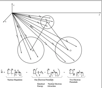
For a graphical explanation of the individual variables, please have a look at the following figure 1. O O S y x z RO RO RS r r1 r 2 3

r_{4 r5} r6

r7 r8

r9

H = 1

2 i n r r i I N + Z_I

One Electron Potentials Two Electron Potentials r r i n n 1 j r

Z_IZ_J r I J N N

+

Nuclear Repulsion

Kinetical Nuclear Electron Energy Attraction

j i

I J i J i

Fig. 1.Schematic view of the Hamiltonian Operator ˆH

describing the electronic structure of SO2, which has

been selected to function as a model-system for all further analysis.

1.2. Decoupling of Electron Repulsion

The coupling of electrons, as given from the last term of equation 2, leads to a correlated motion of electrons, that, explicitly treated, would re-sult in tremendous computational efforts, which might be fairly released, if the following approx-imation is used,

electrons X i electrons X j 1

j~ri ;

~ rjj

electrons X i 2 6 4 Z

~r´

ρ( ~r´

) ~ dr´

~ri;

~r´

+vef f

(~ri )

3

7

5 (3)

with ρ( ~r´

) standing for the Electron Density

around point~r´and v

ef f(~ri

) being an Effective

Potential.

With this approximation, the general n-particle Schr¨odinger equation 1 reduces to its decoupled one-electron form of n4 _{identical one-particle}

equations

2

6 4;

1 2∆;

nuclei X

k

Zk j~r;~rkj

+ Z

~r´ ρ(

~r´ )

~

dr´

~r;

~r´

+vef f (~r

) 3

7

5φk

(~r )=εkφk

(~r )

(4)

where now the φk(~r) are one–electron

wave-functions or molecular orbitals (MO

5

) and

equation 4 once more reflects an eigenvalue problem.

The fundamental property characterizing a mole-cule, the so called one-electron density ρ(

~r ),

is related to the n-particle wave-function

ψel(r~1r~2:::r~n)by

ρ(~r1 )= Z ~ r2 Z ~ r3 ::: Z ~ rn

ψel(~r1

~

r2:::)ψel (~r1

~

r2:::) ~

dr2dr~ 3:::

~

drn

(5)

and takes the special form

ρ(~r) =

electrons

X

i

φi(~r)φi(~r) (6)

for aSlater Determinant.6

1.3. Effective Potential

The practical representation ofvef f( ~r

)in

equa-tion 4 gives rise to two different main stream di-rections in quantum mechanics, where the one is calledDensity Functional Theory 5]and the

other is referred to asHartree Fock Theory 6]

7]. The latter has been used for the present

program we are talking about.

In Hartree Fock theory( HF ) the 3

rd _{and 4}th

term of equation 4 are replaced by the following closed form

4 _{n stands for total number of electrons.} 5 _{Molecular orbitals shall be designatedφ}

kand are said to form an orthonormal set.

6_ψ

el(~r1r~2:::)=Pφ1(~r1)φ2(r~2):::φn(~rn)]wherePmeans Permutation and all is done in order to respectthe Pauli Principle 3], that results from theantisymmetriccharacter of the wave-function.

7_J

jin equation 7 is calledCoulomb OperatorandKjin equation 7 is calledExchange Operator.

8 _{Note, that the Index k refers toφ}

2

6

4 Z

~r´

ρ( ~r´

) ~ dr´

~r

; ~r´

+vef f(~r) 3

7

5

HF

ˆ

=

electrons

X

j

Jj;

1 2Kj

(7)

with the J- and K-terms7_{given by}8

Jj=Jj (~r

)φk (~r

)= 2

6 4 Z

~r´ φj(

~r´ )

1

~r´

;~r

φj( ~r´

) ~

dr´

3

7

5φk

(~r

) (8)

Kj=Kj (~r

)φk (~r

)= 2

6

4 Z

~r´ φj(

~r´ )

1

~r´

;~r

φk( ~r´

) ~

dr´

3

7

5φj (~r

): (9)

Thus the sum over J-terms together with equa-tion 6 is precisely theCoulomb Potential( 3

rd

term of equation 4)and the sum over K-terms

represents a Nonlocal Effective Exchange

Po-tential.

So far we always talked about the electrons only and never spent a word on nuclear charge distri-bution, that theoretically should again be sub-ject to another wave-function and treated in the same quantum way the electrons had been. The neglect of an explicit wave-function for the de-scription of the nuclear charges is due to the fact, that the two wave-functions, for electrons and nuclei either, may be separated into two in-dependent ones, which is commonly known as

theBorn-Oppenheimer Approximation9 2].

1.4. SCF-Procedure

As may be seen from equation 4, the decoupled one–electron Schr¨odinger equation depends on the electron density ρ(~r), which in its turn is

a function of all MOs involved. Therefore all other electrons have a strong influence on the solution of the eigenvalue problem for a partic-ular electron.

This leads to the paradox situation, that one should already know all MOs in order to be able to determine one particular MO explicitly. To overcome this principal problem, equation 4 has to be solved via a so-calledSelf Consistent

Field procedure ( SCF ), which in a sketchy

way may be described as

Set up a first trial densityρ1( ~r

), that will

naturally be far away from the actual phys-ical relevant one.

Solve the eigenvalue problem 4 and thereby

get access to a set of MOs, which in turn results in a better, more realistic new den-sityρ2(

~r

)via equation 6.

Resolve the next eigenvalue problem using

the improved density ρ2(~r) and again get

another, even more improved set of MOs and so on:::until two subsequent sets of

MOs are almost identical to each other and differ only by a predefined small threshold value.

1.5. DIIS-Method

Contrary to our initial report 16] within the

present version, we make use of the

Conver-gence Acceleration of Iterative Sequences. 17],

which is also known as DIIS, meaning Direct

Inversion in Iterative Subspace18], and which

in an oversimplifying way may be regarded as a method capable of drastically reducing the total number of necessary iterations. Thus for our special SO2case, the application of DIIS could

reduce the total number of iterations necessary to achieve self consistency from 44 to 16 and, according to the fact that each individual iter-ation involves the most elaborate task of ERI-computation, the availability of DIIS becomes a limiting factor in terms of cpu-time as well.

1.6. LCAO, Main Problem and Method

According tothe LCAO – approach10_{, the MOs}

are again expanded into a linear combination of atomic orbitals(AO

11

), where the latter might

also simply be calledBasis Functions12

φk(~r)= X

i

ckiϕi

(~r) (10)

9 _{All nuclear centers are considered fixed in space with fixed partial chargesZ} (~rk

)located at those very points in space. 10_{Linear Combination of Atomic Orbitals.}

11 _{Atomic orbitals shall be designatedϕ}

i.

12 _{Basis functions are those widely known 1s, 2s, 2px, 2py, 2pz}

:::orbitals for the description of one-electron atomic systems

Schematic Representation of SO2

CenterElement 1S 2O 3O

Cntr. Shll.Typ (1)S (2)SP (3)SP (4)SP (5)S (6)SP (7)SP (8)S (9)SP (10)SP

Basisf.Typ 1S 2S 6S 10S 14S 15S 19S 23S 24S 28S

3Px 7Px 11Px 16Px 20Px 25Px 29Px

4Py 8Py 12Py 17Py 21Py 26Py 30Py

5Pz 9Pz 13Pz 18Pz 22Pz 27Pz 31Pz

Table 1.Shell concept explained at the model-molecule SO2, that has been used for further analysis.

and the basis functionsϕiare again expanded in

a series overPrimitive Gaussiansχj

ϕi(~r

)=

X

j

dijχj (

~r

) (11)

which typically are Cartesian Gaussian

Func-tions located at some place (AxAyAz) in

space13 ₈

] 9].

χj(~r

)=Nj(x;Ax)

l

(y;Ay)

m

(z;Az)

n _e;αj(~r; ~

A) 2

(12)

The main problem for SCF-calculations is the evaluation of the ERIs, the Electron Repulsion

Integrals, that are 6-dimensional, 4-center

inte-grals over the basis functionsϕ.

ERI=

Z

~

r1

Z

~

r2

ϕi(

~

r1)ϕj (~r1

)

1

j~r2;~r1 j

ϕk(

~

r2)ϕl( ~

r2) ~

dr1dr~

2

(13)

There are various ways to compute ERIs 10]

11] 12], but the method used in the present

program is the recursive method14_{described by}

Obara and Saika 12].

1.7. Shell Concept and Model-Molecule SO2

Without any intention of going into further de-tails, we just want to outline, at least basically, the principal scheme behind the recursive con-struction of ERIs due toObara and Saika 12].

For all further report we present data for a simple molecule, that has been used as a certain kind

of reference – SO2 in particular. A schematic

representation of the molecule is given in ta-ble 1. The applied basis function specifica-tion has been the standard 6-31G basis-set 13]

14]. The main advantage of this 6-31G

basis-set is, that there exist cross-contracted shells, e.g. SP-contracted shells, which will utilize the same exponential factor(α in equation 12)for

S-type basis functions as well as P-type basis functions15_{, and hence will offer a chance to}

calculate the more complicated ERIs, that con-tain P-type basis functions, in an recursive way from easily generated pure S-type ERIs. As stated above, ERIs are 4-center integrals, and therefore we will have to combine 4 centers together with the according contracted shells to determine how many ERIs may be built in one subsequent, recursive subprocess. For example, consider the center-quartet 1 1 2 3 , then one possible combination of contracted shells would be(2)(3)(5)(9)

16_{, with the basic S-type}

ERI made up from basis functions 2 6 14 24, and after initial calculation of this basic S-type ERI, a total number of 63 related ERIs may be derived recursively, such as 2 6 14 25, 2 6 14 26, 2 6 14 27, 2 7 14 24, 2 7 14 25, 2 7 14 26

:::5 9 14 27.

2. Performance Analysis

2.1. General Status

To shed some light onto critical regions of our program, we have used performance

measure-13 _{An S-type basis function will consist of primitive gaussians withl}

= m= n=0, a P-type however of primitives with

l+m+n=1, which may be solved at 3 different ways, eitherl=1 andm=n=0, orm=1 andl=n=0, orn=1 and

l=m=0. D-type specification will likewise bel+m+n=2 and similarly F-typel+m+n=3. 14 _{All complicated ERI-types}

(l+m+n>0)may be deduced from the easier computed(SiSjjSkSl)type. 15_{For example, basis functions 6, 7, 8 and 9 of contracted shell}

(3)at center 1 will all have the same exponentα.

16 _{There are 90 possible combinations of relevant contracted shells within this particular center-quartet and we have only picked}

ment tools, as provided on a SGI-Power Chal-lenge/R10000(194 MHz)running IRIX 6.2.

Some insight into the basic events of the R10000 processor for some specific program execution may be gained by using the shell-command

per-fex -a a.out. Then a table is given, which

repre-sents a listing of total counts of various events, such as 2nd _{level data cache misses, or issued}

loads, or graduated loads, or:::that happened

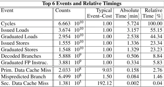
during program execution and thus17a relative weighting of critical events may be done to no-tice some basic bottlenecks. A listing of the top 6 events during our SCF-process together with some relative numbers of highly sensitive events is given in table 2.

2.1.1. Interpretation

At least no principal performance bottlenecks were encountered, especially when looking at highly sensitive events, such as data cache misses and mispredicted branches. So we don’t think that this application suffers from serious perfor-mance problems, which could be solved at the programmer’s level.

2.2. Main Time Consuming Modules

The other thing we were highly interested in, was to select those subroutines and functions, that play the main part during program execu-tion as far as cpu-time is concerned. Therefore we did some performance measurement on the SGI-Power Challenge/R10000(194 MHz)

run-ning IRIX 6.2, namelyssrun -[pcsampl, ideal,

usertime] a.out, which all produce ordered

list-ings of the involved modules according to their fraction in the total cpu-time.

No matter which of the three optional parame-ters were selected in particular, it always turned out that 99.7 % of the total cpu-time was spent

inSubroutine FMAT, which is our module for

ERI–computation.

3. Parallelization

As has become clear from the previous sec-tion 2.2, our primary goal for parallelizasec-tion purposes had to be subroutine FMAT — the ERI-calculation module.

For the first approach we used PVM 3.318_{for a}

host–node model due to the MPMD scheme19_,

where the outermost loop20 _{within subroutine}

FMAThad been split and partitioned over a cer-tain range of nodes.

Top 6 Events and Relative Timings

Event Counts Typical Absolute Relative

Event–Cost Time min] Time %]

Cycles 6.663 1010 1.00 5.724 100.00

Issued Loads 3.674 1010 1.00 3.157 55.15

Graduated Loads 2.954 1010 1.00 2.538 44.34

Issued Stores 1.555 1010 1.00 1.336 23.34

Graduated Stores 1.548 1010 1.00 1.329 23.23

Decoded Branches 5.888 109 _{1.00 0.506 8.84}

Graduated FP Instruc. 3.881 109 _{1.00 0.334 5.83}

Prim. Data Cache Miss 2.033 108 9.03 0.158 2.76

Mispredicted Branch 6.499 108 1.50 0.084 1.46

Sec. Data Cache Miss 1.381 105 192.12 0.002 0.04

Table 2.Relative timings of specific hardware counters on R10000, SGI for one SCF-process completion.

17 _{After multiplying those absolute counts with specific event–cost–figures.}

18 _{Rel. 11 on the alpha-cluster made up of equal dec 3000 nodes, Rel. 10 on the SGI Power Challenge R10000.} 19 _Multiple

Wall Clock Times and Speed–Up

Number of Nodes Wall Clock Time min] Speed Up

Dec 3000 Cluster 1 – sequential 46:12

Dec 3000 Cluster 2 32:03 1.44

Dec 3000 Cluster 4 21:00 2.20

Dec 3000 Cluster 8 13:34 3.46

Table 3.Wall-clock times for parallel SCF on Dec 3000 cluster for different number of nodes and derived speed-up parameter. Arithmetic average partitioning scheme.(Without DIIS !)

To begin with, we present data(table 3)

result-ing from a simple arithmetic average partition-ing scheme, where each of the involved nodes got to work on a certain subset of center quartets and the number of individual items within this subsets was derived by simply dividing the total number of all possible center quartets through the number of nodes involved. ( partitioning

scheme also shown on left side of table 4)

3.1. Load Balancing

After realizing the poor speed up factors ob-tained from the initial, simple arithmetic aver-age partitioning scheme ( left side of table 4

), we went one step further and introduced a

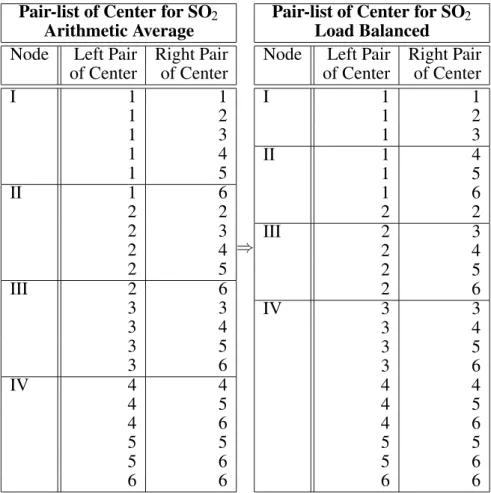
pre-scanning subroutine, with which we could estimate the net work to be done. This means, that instead of actual calculating ERIs, we just increment a counter variable in the according section of the program, where usually the re-cursive relations for the computation of ERIs come into play, and thus we end up with a rep-resentative number for the total computational work to be done, which may be divided through the number of nodes involved and in a sub-sequent repetition of the dummy loops it may be useful to assign the upcoming center quar-tets to the same node-specific pair-list as long as the mentioned fraction total work counter_{number of nodes} is not reached. In this way we were able to build so called load-balanced pair-lists, that represented the outermost loop over center quartets. The latter scheme gave rise to the following pair-lists of center21

( right side of table 4 ) and

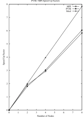
a summary of corresponding speed-up data for the likewise improved parallel versions is given in table 5 for the PVM version as well as for the MPI version both executed on the SGI-Power

Challenge/R10000 (194 MHz). A graphical

representation of table 5 is given in figure 2.

0 1 2 3 4 5 6 7 8

0 1 2 3 4 5 6 7 8

Speed Up Factor

Number of Nodes PVM / MPI Speed Up Factors

MPI PVM Ideal

Fig. 2.Comparison of Speed-up Factors for PVM and MPI approach.

4. Discussion

4.1. Dominance of Heavy Atoms like S

As might have become clear from section 1.7 all center quartets containing atom S(or related

pairs of centers – 1, 2, 3) will result in larger

numbers of according ERIs, because S is built up from 3 cross contracted SP-shells —(2),(3)

21 _{According to the specification done in table 1 pair 1 will be 1 1 , 2 is 1 2 , 3 is 1 3 , 4 is 2 2 , 5 is 2 3 and 6 is}

and(4)— whereas the remaining two O-atoms

are only built up from 2 SP-shells, which is also noticed in table 4 ( right side ), because node

IV for example is mainly working on ERIs not containing atom S, thus effecting 10 different center quartets, whereas node I may only work on 3 center quartets but these will always in-clude atom S and the work of both nodes should still be almost equal to each other.

4.2. Amdahl’s Law and a Detailed Picture of the Time Distribution within the Parallel Process

According toAmdahl’s Law

SpeedUp

1

s+

1;s

Ncpu

(14)

withs standing for the serial fraction and Ncpu

for the number of nodes, we should obtain

speed up values almost equal to the number of nodes involved, if we assume that s is suffi-ciently small and that communication may be neglected. From section 2.2 we may conclude thats =0:003, which leads to theoretical speed

up values of 1.994 for 2 nodes, 3.964 for 4 nodes and 7.836 for 8 nodes.

Nevertheless our measured speed up values as represented in table 5 differ quite a lot from those theoretical values, which is due to the fact, that despite serious efforts to enable a well balanced work distribution one cannot over-come the principal block structure for ERI-computation( section 1.7 ). This means, that

even after building load balanced pair-lists all nodes will still have to work on slightly varying fractions of partial work, that are comparable to each other, but not exactly equal.22

So after 3 nodes, for example, have already fin-ished their partial work, node IV may still be busy completing its last center quartet, which

Pair-list of Center for SO2

Arithmetic Average

Node Left Pair Right Pair of Center of Center

I 1 1

1 2

1 3

1 4

1 5

II 1 6

2 2

2 3

2 4

2 5

III 2 6

3 3

3 4

3 5

3 6

IV 4 4

4 5

4 6

5 5

5 6

6 6

)

Pair-list of Center for SO2

Load Balanced

Node Left Pair Right Pair of Center of Center

I 1 1

1 2

1 3

II 1 4

1 5

1 6

2 2

III 2 3

2 4

2 5

2 6

IV 3 3

3 4

3 5

3 6

4 4

4 5

4 6

5 5

5 6

6 6

Table 4.Arithmetic average and load-balanced partitioning scheme of the outermost loop over center quartets into node-specific pair-lists of center for SO2— 4 nodes considered.

22_{Like the area of a puzzle can be divided into a number of almost equal partial areas, but not into exactly equal partial areas,}

Wall Clock Times and Speed–Up

Number of Nodes Wall Clock Time sec] Speed Up

SGI Pow.Chll. PVM 1 – sequential 268.19

SGI Pow.Chll. PVM 2 149.78 1.79

SGI Pow.Chll. PVM 4 88.66 3.03

SGI Pow.Chll. PVM 8 44.40 6.04

SGI Pow.Chll. MPI 1 – sequential 252.51

SGI Pow.Chll. MPI 2 132.50 1.91

SGI Pow.Chll. MPI 4 86.10 2.93

SGI Pow.Chll. MPI 8 43.28 5.83

Table 5.Wall clock times for parallel DSCF for either PVM 3.3 or MPI approach on SGI-Power Challenge/R10000 (194 MHz)for different number of nodes and derived speed-up parameter. Load balanced partitioning scheme.

.. ..

.. ..

0.45 15.56 0.2 15.56 0.25

0.23 15.55

0.2 15.56

0.45

MASTER NODE 1

15 x

15 x D I I S

D I I S T

F M A T

F M A

P A R T P A R T

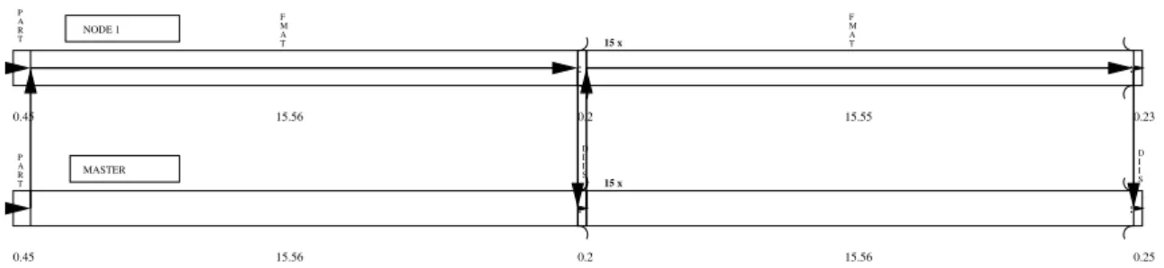
Fig. 3.Cpu-time distribution to the different threads for the MPI-approach of the DSCF calculation of SO2

considering 1 master and 1 node process. The execution cycle is indicated by the arrows.

forces all other 3 nodes to stay idle in the mean-time and thus induces an artificial enlargement of the serial fraction of program execution. Ac-cording to this, in order to get a closer picture of how the cpu-time is spent in the different parallel tasks, we inserted time stamps in the source code of the program, so that each of the working nodes could report its own individual time it spent on the execution of its partial work. The authors found it most useful to utilize the

dtime() function, that returns the actual

cpu-time since the last call to dcpu-time(). In this

man-ner we actually could visualize the aforemen-tioned latency-effect due to the undestroyable block-structure of the different nodes concern-ing their individual partial work to perform and a summary of the obtained cpu-time-flowcharts is given within figures 3, 4 and 5.

4.3. PVM versus MPI

After treating the PVM program the same way and inserting the same kind of time stamps there, we noticed slight differences between the MPI and the PVM approach concerning cpu-time distribution, which surprisingly was not due to communication impairment in the PVM task.

..

..

.. ..

..

D I I S

..

0.45 MASTER P

A R T

7.57

7.57 0.5 0.2 0.75

P A R T 0.45

0.45 8.05

T F M A NODE 2

D I I S 15 x

15 x 15 x

0.2

0.75 NODE 1

P A R

T T

F M A

T F M A

T F M A 7.57

7.57

8.05

0.5 0.2

0.25

Fig. 4.Cpu-time distribution to the different threads for the MPI-approach of the DSCF calculation of SO2

considering 1 master and 2 node processes. The execution cycle is indicated by the arrows.

The effect decreases with increasing number of nodes and thus becomes less harmful for the ac-tual interesting jobs. An overview of the differ-ent influence of the PVM-delay is given within figures 6, 7, 8 and 9.

4.4. Neglectable Influence of the Additional Partitioning Module

.. .. .. .. .... .. .. .. .. .. 0.45 MASTER P A R T P A R T 0.45 0.45 NODE 1 P A R T 0.45 P A R T 2.98 2.98 0.45 P A R T 3.71 3.88 NODE 2 5.06 NODE 3 NODE 4 0.2 15 x 2.37 1.63 1.48 0.29 15 x 15 x 15 x 15 x T

F M A T F M A T F M A D I I S D I I S 5.06 T F M A 3.71 1.68 0.34 0.2 2.98 2.98 2.41 3.88 1.53 0.16 0.16 1.2 1.2 0.7 0.7 .. .. .. .. .. .. .. .. .. .. .. .. .. .. .. .. .. MASTER P A R T P A R T P A R T 1.23 1.23 1.45 0.2 P A R T 1.85 NODE 5 P A R T 1.90 0.5 P A R T 1.93 P A R

T NODE 1

2.46

P A R

T NODE 7

2.45

P A R

T NODE 8

2.48 1.5 1.23 1.23 1.3 1.45 0.2 0.9 1.85 0.9 1.90 0.9 1.93 NODE 2 NODE 3 NODE 4 15 x 15 x 15 x 15 x NODE 6 15 x 0.2 0.2 2.45 0.2 2.48 0.3 2.46 15 x D I I S 0.2 0.4 0.4 0.5 1.3 0.9 0.2 0.2 1.5 0.9 0.9 0.3 15 x 15 x 15 x 0.4 0.4 0.4 0.4 0.4 0.4 0.4 0.4 0.4

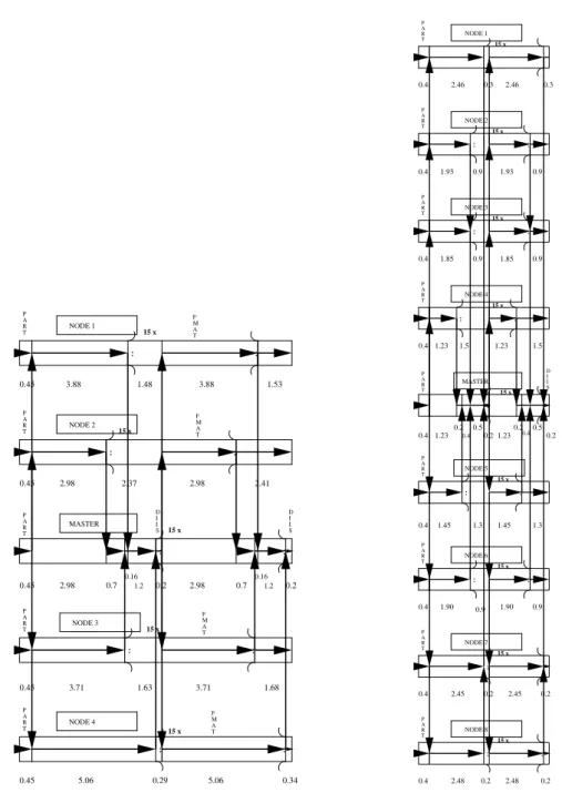
Fig. 5.Cpu-time distribution to the different threads for the MPI-approach of the DSCF calculation of SO2

considering 1 master and 4 node processes(left)1 master and 8 node processes(right). The execution cycle is

indicated by the arrows.

this additional load balancing subroutine, that from the point of view of the SCF process is re-garded artificial and not necessary and therefore should be kept at a minimum expensive level. It turned out, that the actual cpu-time spent for this additional task was 0.33 sec, which, even for the fastest run, is only a percentage of 0.76 %.

4.5. Conclusion

Recursive ERI-computation according toObara

and Saika 12]cannot be done in 100 % parallel

tasks 1 x

16 x

5 10 15 cpu t i m e [s]

m a s e r t

n o d e 1

MPI

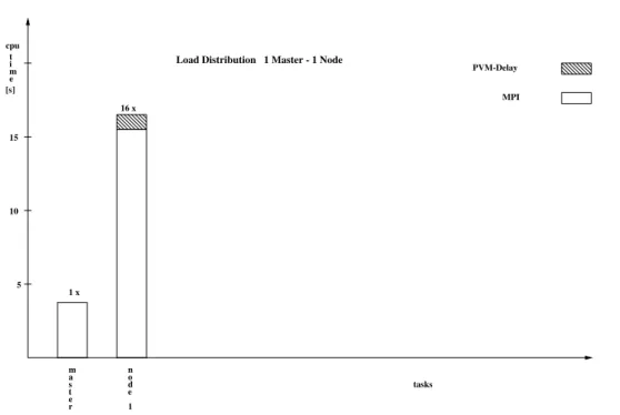
Load Distribution 1 Master - 1 Node

PVM-Delay

Fig. 6.Comparison of the cpu-time the different nodes have to spend on performing their partial work and indication of the effect of PVM-delay. (1 master 1 node)

tasks 1 x

5 10 15 cpu t i m e [s]

m a s e r t

MPI

16 x 16 x

n o d e 1

n o d e 2

Load Distribution 1 Master - 2 Node

PVM-Delay

Fig. 7.Comparison of the cpu-time the different nodes have to spend on performing their partial work and indication of the effect of PVM-delay. (1 master 2 nodes)

References

1] SCHRODINGER¨ , E. Quantisierung als

Eigenwert-problem. Annalen der Physik.79,80,81(1926).

2] BORN, M., OPPENHEIMER, R., Zur Quantentheorie

der Molek¨ule. Annalen der Physik.84(1927)457.

3] PAULI, W., Exclusion Principle and Quantum

Me-chanics. Neuchatel, Griffon, 1st. Ed., Nobel Prize Lecture.(1947).

4] SLATER, J.C., The Self Consistent Field for

Molecules and Solids: Quantum Theory of Molecules and Solids Mc Graw-Hill, New York,

4(1974).

5] PARR, R.G., YANG, W., Density Functional Theory

of Atoms and Molecules. Oxford University Press, New York,(1989).

6] HARTREE, D.R., Proc. Camb. Phil. Soc.,24(1928)

tasks 1 x

5 10 15 cpu t i m e [s]

m a s e r t

MPI

n o d e 2

n o d e n

o d e 1

n o d e

3 4

16 x

16 x

16 x

16 x

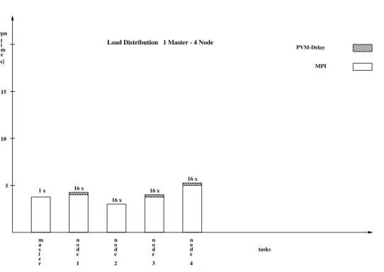
Load Distribution 1 Master - 4 Node

PVM-Delay

Fig. 8.Comparison of the cpu-time the different nodes have to spend on performing their partial work and indication of the effect of PVM-delay. (1 master 4 nodes)

1 x 5

10 15 cpu t i m e [s]

m a s e r t

MPI

n o d e 2 n

o d e 1

n o d e 4

tasks n

o d e 3

n o d e

n o d e

n o d e

n o d e

5 6 7 8

16 x

16 x

16 x 16 x 16 x

16 x 16 x 16 x

Load Distribution 1 Master - 8 Node

PVM-Delay

Fig. 9.Comparison of the cpu-time the different nodes have to spend on performing their partial work and indication of the effect of PVM-delay. (1 master 8 nodes)

7] FOCK, V., N¨aherungsmethoden zur L ¨osung des

Quantenmechanischen Mehrk¨orperproblems. Z. Physik,61(1930)12662(1930)795.

8] DAVIDSON, E.R., FELLER, D., Basis Set Selection

for Molecular Calculations. Chem. Rev.,86(1986)

681–696.

9] SHAVITT, I., The Gaussian Function in Calculations

of Statistical Mechanics and Quantum Mechanics. Methods in Computational Physics, academic, New York,2(1963)1–44.

10] SAUNDERS, V.R., An Introduction to

Molecu-lar Integral Evaluation. Computational Techniques in Quantum Chemistry and Molecular Physics, Reidel–Dordrecht(1975)347–424.

11] MCMURCHIE, L.E., DAVIDSON, E.R., One–and

Two–Electron Integrals over Cartesian Gaussian Functions. J. Comp. Phys.26(1978)218–231.

12] OBARA, S., SAIKA, A., Efficient recursive

13] HEHRE, W.J., DITCHFIELD, R., POPLE, J.A., J. Chem.

Phys.56(1972)2257.

14] FRANCL, M.M., PETRO, W.J., HEHRE, W.J., BINK

-LEY, J.S., GORDON, M.S., DEFREES, D.J., POPLE, J.A., J. Chem. Phys.77(1982)3654.

15] GEIST, A., BEGUELIN, A., DONGARRA, J., JIANG,

W., MANCHEK, R., SUNDERAM, V., PVM: Parallel Virtual Machine. A Users’ Guide and Tutorial for Networked Parallel Computing MIT Press(1994).

16] H ¨OFINGER, S., STEINHAUSER, O., ZINTERHOF, P.,

Performance Analysis and Derived Parallelization Strategy for a SCF Program at the Hartree Fock Level. Lect. Nt. Comp. Sc.1557(1999)163.

17] PULAY, P., Convergence Acceleration of Iterative

Sequences. The Case of SCF Iteration. Chem. Phys. Letters73(1980)393–398.

18] PULAY, P., Improved SCF Convergence

Accelera-tion. J. Comp. Chem.3, No.4(1982)556–560.

Received:May 15, 1999

Accepted in revised form:January 21, 2000

Contact address:

Siegfried H¨ofinger and Othmar Steinhauser Institute for Theoretical Chemistry Molecular Dynamics Group University of Vienna W¨ahringerstr. 17, Ground Floor, A-1090 Vienna Austria e-mail:fsh,[email protected]

http://www.mdy.univie.ac.at

Peter Zinterhof Institute for Mathematics University of Salzburg Hellbrunnerstr. 34 A-5020 Salzburg Austria e-mail:[email protected] http://www.mat.sbg.ac.at

SIEGFRIEDHOEFINGERreceived the M.S. degree in biochemistry from the University of Vienna in 1996 and the Ph.D. degree in theoretical chemistry from the University of Vienna in 1998. In 1999 he was a postdoctroal research fellow at the IGBMC, the Institut de Genetique et de Biologie Moleculaire et Cellulaire in Strasbourg, where he worked in the lab of Dr. Thomas Simonson on the development of new algorithms for the large scale dielectric response in proteins. Currently he is a research fellow at the Institute for Theoretical Chemistry and Structural Biology of the University of Vienna. His scientific interests include parallel algorithms in quantum chemistry, high performance computing on multiprocessor architectures and algorithm design and analysis of programs used for ab-initio simulations in computational chemistry.

OTHMARSTEINHAUSERgraduated from the University of Vienna in 1975 with a Ph.D. in physics. After promotion sub auspiciis praesidentis he worked as a research assistant at the Institute for Theoretical Chemistry, University of Vienna and became a DFG-assistent at the Institute for Physical Chemistry, University of Karlsruhe in 1979. After habilitation in theoretical chemistry in 1984 he became Assistant Professor at the Johannes-Gutenberg University of Mainz in 1987 and Full Professor of chemical molecular dynamics at the Institute for Theoretical Chemistry, University of Vienna in 1991. He is head of the Computing Center of the University of Vienna since 1992. His current research interests include computer simulation on the structure and dynamics of solvated biomolecules, algorithm design for the treatment of electrostatic in-teractions in biomolecules, multiprocessor computer architectures and parallel machines.

PETERZINTERHOFis director of the Research Institute for Software Technology and chair of the Department of Scientific Computing at Salzburg University, Austria. He holds a full professorship of mathe-matics and theoretical computer science. His research interests include number-theoretical numerics, parallel and distributed processing, im-age processing, and stochastics. He is project leader of several national

(FWF-funded)and international(INTAS-funded)research projects and