Linear Combination and Reliability of Generalized Logistic Random Variables

Vol. 12, No. 3, 2019, 722-733

ISSN 1307-5543 – www.ejpam.com Published by New York Business Global

Linear combination and reliability of generalized logistic

random variables

Luan C. de S. M. Ozelim1,∗, Pushpa N. Rathie2

1_{Department of Civil and Environmental Engineering, University of Brasilia, Brasilia- DF,}

70910-900, Brazil

2 _{Department of Statistics, University of Brasilia, Brasilia- DF, 70910-900, Brazil}

Abstract. Experimental random data, in general, present a skewed behaviour. Thus, asymmet-rical generalized distributions are of interest. The generalized logistic distributions (GLDs) are good candidates to model skewed data because their probability density functions (p.d.f.) and characteristic functions are mathematically simple. In this paper, exact expressions in terms of the H-function are, for the first time, derived for the p.d.f. and for the cummulative distribution function of the linear combination of GLDs of type IV with different location, scale and shape

parameters. Also, exact and approximate expressions are derived forR=P(X < Y). Numerical

examples illustrate the correctness of the expressions derived.

2010 Mathematics Subject Classifications: 33C60

Key Words and Phrases: Generalized Logistic Distribution, Mellin Transform, Fourier Trans-form, H-function, Reliability

1. Introduction

Modelling nature is by no means a trivial task. At first, scientists have to observe how a given phenomenon occurs and then, by means of physically justifiable premises, propose a model which is able to predict the outcomes of such phenomenon when some important inputs are known. Over the last half century, the scientific community started to model both the inputs and outcome of such models as random variables. Thus, the algebra of random variables has become increasingly of interest to not only pure but also applied scientists.

Instead of modelling failure as stresses overcoming a given strength threshold, a prob-abilistic approach enables one to calculate the probability of failure. The latter approach may lead to cost reduction and time consumption in the implementation of a given project. [13]

∗

Corresponding author.

DOI: https://doi.org/10.29020/nybg.ejpam.v12i3.3444

Email addresses: [email protected](L. C. de S. M. Ozelim), [email protected](P. N. Rathie)

The application of reliability measures of the type R = P(X < Y), where X is the stress to which a given structure of strength Y is subjected, have many applications in various areas, including quality control, engineering statistics, reliability, medicine, psychology, biostatistics, stochastic precedence, and probabilistic mechanical design [9, 10]. For example, if X represents the maximum pressure caused by flooding and Y represents the strength of the leg of a bridge on a stream, then R is the probability that the bridge will resist [7].

On the other hand, for medical applications, let X and Y represent the control and treatment groups, respectively. Then R measures the treatment effect [7, 18]. Alterna-tively, in the cases of diagnostic tests used to distinguish between diseased and non-diseased patients, the area under the receiver operating characteristics (ROC) curve, based on the sensitivity and the complement to specificity at different cut-off points of the range of possible test values, is equal toR [16, 18].

Besides, in the ecotoxicological risk assessment literature, Ris also employed to quan-tify risk [8]. Thus, it is clear that studying reliability measures of the typeR=P(X < Y) is fundamental to various areas of science. In this regard, the estimation ofRis of interest to provide information in decision processes. It is common for authors to assume that X

and Y belong to a certain family of probability distributions with unknown parameters and then to consider the estimation problem of the reliabilityR[7]. One may check [7] and the references therein for estimation problems related to exponential, uniform, generalized exponential, generalized gamma, Burr, gamma and beta distributions.

Being able to build not only estimates but also the exact value ofRwhen the statistical distribution of the variables involved are known is then important. Besides considering the random variables (RVs) previously cited, it is important to obtain the exact value of

R for more general RVs. In the present paper, generalized logistic random variables are studied.

Statistical models of the logistic type have been applied to all sorts of pure and applied problems in Statistics. This comes from the fact that logistic models are flexible, being able to mimic normality as well as show skewness in some generalized models. Applications of this kind of random variable are easily seen in the literature. A complete study has been recently performed in [12]. For example, regarding applied scientists, [4] employed generalized logistic models to perform flood analysis in partial duration series.

On the other hand, regarding pure statistics papers, [19] discussed the parameter es-timation for a certain type of generalized logistic distribution. Also, [3] obtained approxi-mate maximum likelihood estimation for some generalized logistic distributions. Besides, [1] performed a comparative study of the techniques available for the estimation of the generalized logistic distribution parameters.

Consider a random variable S. LetS follow a generalized logistic distribution of type IV, from now on called GLD. Also, let one consider a location parameter µ∈_R, a scale parameter σ > 0 and two shape parameters α and β such that α, β > 0. One says

f(x;σ, µ, α, β) = 1

B(α, β)

e−β(x−σµ)

σ[1 +e−(x−σµ)]α+β

, ∀x∈R, (1)

whereB(α, β) is the Beta function, defined as:

B(α, β) =

Z 1

0

tα−1(1−t)β−1dt= Γ(α)Γ(β)

Γ(α+β). (2)

In (2), Γ(x) stands for the Gamma function defined as:

Γ(x) =

Z ∞

0

tx−1e−tdt. (3)

Despite being constantly considered in pure and applied sciences, no closed-form com-pact representation for the sum of independent not identically distributed generalized logistic random variables has been presented yet. In the present paper, the linear com-bination of generalized logistic random variables with different location, scale and shape parameters is given, in a compact form, in terms of the H-function. This latter function is a generalized hypergeometric special function whose importance has been widely recog-nized. In special, [17] discusses the central role of this function to the study of the algebra of random variables. Besides the pure statistical applications where the linear combination itself is sought, reliability models can also be derived based on the latter by noticing that

R=P(X < Y) =P(X−Y <0).

As discussed, mathematical procedures are used to estimate R. Regarding logistic RVs, for example, [14] proposed methods of estimation of the shape parameters of the generalized logistic distribution and of P(Y < X), when X and Y were independent random variables from two distributions having the same scale parameters but different shape parameters.

More recently, [2] derived estimators for R when both the distributions compared are generalized logistic. The authors considered the estimation of R, whenX andY are both two-parameter generalized logistic distribution with the same unknown scale but different shape parameters or with the same unknown shape but different scale parameters. They also considered the general case when the shape and scale parameters are different. In [2] the maximum likelihood estimator of R and its asymptotic distribution are obtained and it is used to construct the asymptotic confidence interval of R. Besides, [5] studied the estimation of two measures of reliability for generalized half logistic distributions.

One of the purposes of the present paper is to provide exact and approximate formulas

for reliability measuresR=P(

N1

P

i=1

Xi< N2

P

j=1

Yj), whenXi,i= 1, ..., N1andYj,j= 1, ..., N2

Considering the linear combination of RVs instead of simply R = P(X < Y) is of interest because in many applications, the stress and strength are described in terms of other random variables. For example, the strength of a given geomaterial may be obtained by means of the Mohr-Coulomb failure criterion. Mathematically, this criterion may be represented as [6]:

τ =σtan(φ) +c (4)

whereτ,σ and care the shear, normal, and cohesion stresses, respectively. When both σ

andcare considered as RVs, it can be seen from (4) that the shear resistanceτ is nothing but the linear combination of the other random variables, as the internal friction angleφ

may be considered constant.

Obtaining the linear combination is, thus, more interesting than simply expressing

P(X < Y), as the results are more general. For example, in [15], linear combinations,

products and ratios of t Random Variables were studied, therefore all the theoretical and mathematical basis for studying reliability measures for that specific type of random variable is presented. To familiarize the reader, the definition of the H-function and its Mellin Transform are given in the next section.

2. The H-function

The H - function (see [11] ) is defined, as a contour complex integral by

H_p,qm,n

z

(a1, A), . . . , (an, An), (an+1, An+1), . . . , (ap, Ap)

(b1, B1), . . . , (bm, Bm), (bm+1, Bm+1), . . . , (bq, Bq)

= 1 2πi Z L m Y j=1

Γ(bj+Bjs) n

Y

j=1

Γ(1−aj−Ajs)

q

Y

j=m+1

Γ(1−bj−Bjs) p

Y

j=n+1

Γ(aj+Ajs)

z−sds, (5)

where Aj and Bj are positive quantities and all the aj and bj may be complex. The

contour L runs from c−i∞ toc+i∞ such that the poles of Γ(bj +Bjs), j = 1, . . . , m

lie to the left ofL and the poles of Γ(1−aj −Ajs), j= 1, . . . , n lie to the right ofL.

The Mellin transform of the H -function is given by

Z ∞

0

xs−1H_p,qm,n

cx

(ap, Ap)

(bq, Bq)

dx=

c−s m

Y

j=1

Γ(bj+Bjs) n

Y

j=1

Γ(1−aj−Ajs)

q

Y

j=m+1

Γ(1−bj−Bjs) p

Y

j=n+1

Γ(aj +Ajs)

z−s. (6)

3. The Linear Combination of N GLDs

A brief description of the problem is presented and its solution is derived in this section.

3.1. Problem Statement

Let Xi ∼GLD(µi, σi, αi, βi). Then, one seeks the probability density function of the

random variable:

Z =

N

X

i=1

biXi (7)

wherebi,i= 1, ..., N are real numbers.

At first, one may obtain the p.d.f. of the linearly scaled distributions biXi. This can

be easily done by considering the Jacobian rule as presented in [17]. Thus, when Xi ∼ GLD(µi, σi, αi, βi), the transformed random variable biXi has a p.d.f. mathematically

represented as:

fbiXi(x;σi, µi, αi, βi, bi) =

1

|bi|σiB(αi, βi)

e−βi(

x−_biµi

biσi )

[1 +e−(

x−_biµi

biσi )_]αi+βi

, ∀x∈R, (8)

This way, by using (7) and (8), the variable Z can be rewritten as the sum of the random variables Yi, with Yi = biXi. To get a closed form exact probability density

function of the random variable Z, one shall first proceed to obtain of the characteristic functions of the random variablesYi,i= 1, ..., N.

3.2. The Characteristic Function of Yi, i= 1, ..., N

The characteristic function of a given random variable can be obtained by calculating the Fourier transform of its probability density function. The characteristic function of a GLD random variable is widely known in the literature [12]. On the other hand, in order to better understand the scaling process performed to generate the variableYi =biXi, the

characteristic function of Yi shall be obtained explicitly. This way, by means of (8), the

characteristic function φi(t) (CF) for the random variablesYi,i= 1, ..., N is given by:

φi(t) =

1

σi|bi|B(αi, βi)

∞

Z

−∞

ejtx e

−(x−µibi) σibi

1 +e− (x−_µibi)

σibi

αi+βidx, (9)

wherej =√−1.

On substituting r=e− (x−_µibi)

σibi _/

1 +e− (x−_µibi)

σibi

φi(t) =

ejtbiµi

B(αi, βi)

1

Z

0

rβi−jtσibi−1_(1−r)αi+jtσibi−1_{dr. (10)}

By considering the Beta function definition in (2), (10) becomes:

φi(t) =

ejtbiµi

B(αi, βi)

B(βi−jtσibi, αi+jtσibi). (11)

Since the characteristic function of the sum of independent random variables is the product of the individual characteristic functions [17], the CF of the random variable Z,

φZ(t) , is given by:

φZ(t) = N

Y

i=1

ejtbiµi

B(αi, βi)

B(βi−jtσibi, αi+jtσibi)

. (12)

The probability density function of the random variable Z is obtained by the Fourier transform as described in the next subsection.

3.3. The Probability Density Function of the Linear Combination of GLD Variables

Being the CF of the random variable Z known, by means of the inversion formula for Fourier transform, one shall get that the probability density function of Z, fZ(x).

By considering the alternative representation of the Beta function in terms of Gamma functions presented in (2), fZ(x) can be expressed as:

fZ(x;σ, µ, α, β, b) =

1 2π

∞

Z

−∞

e

−jt x−PN i=1

biµi !

N

Y

i=1

Γ(βi−jtσibi)Γ(αi+jtσibi)

Γ(αi)Γ(βi)

dt, (13)

where σ, µ, α,β and b represent the vectors of scale, mean and shape parameters and coefficients, respectively.

It is possible to transform the real integral in (13) into a contour integral by the variable change jt=s. In order to represent the equivalent contour integral in terms of the H-function, one has to split the coefficients bi in positive and negative groups such

that bi ≥ 0, for 1 ≤bi ≤ N1 and bi ≤0, for N1+ 1 ≤ bi ≤ N. This way, by means of

the transformed complex integral and the definition of the H-function in (5), (13) can be rewritten as:

fZ(x;σ, µ, α, β, b) =

1

QN

i=1Γ(αi)Γ(βi)

×H_N,NN,N 

e

x−PN

i=1

biµi

(1−β1, σ1b1), ...,(1−βN1, σN1bN1),(1−αN1+1, σN1+1|bN1+1|), ...,(1−αN, σN|bN|) (α1, σ1b1), ...,(αN1, σN1bN1),(βN1+1, σN1+1|bN1+1|), ...,(βN, σN|bN|)



.

Equation (14) provides a closed form exact representation for the probability density function of the linear combination of GLD random variables,valid forσi, αi, βi>0,µi ∈R

and bi ∈ R, i = 1, ..., N. The cumulative distribution function is given in the next

subsection.

3.4. The Cumulative Distribution Function of the Linear Combination of GLD Random Variables

The cumulative distribution function of the random variable Z,FZ, whose p.d.f. is in

(14), is given by:

FZ(x;σ, µ, α, β, b) =

1

QN

i=1Γ(αi)Γ(βi)

× (15)

×Rx

−∞H

N,N N,N  e

x−PN

i=1

biµi

(1−β1, σ1b1), ...,(1−βN1, σN1bN1),(1−αN1+1, σN1+1|bN1+1|), ...,(1−αN, σN|bN|)

(α1, σ1b1), ...,(αN1, σN1bN1),(βN1+1, σN1+1|bN1+1|), ...,(βN, σN|bN|)

 dx.

Equation (16) is nothing but nested real and contour integrals. By interchanging the order of integration, (16) becomes [11]:

FZ(x;σ, µ, α, β, b) =

1

QN

i=1Γ(αi)Γ(βi)

× (16)

×H_NN,N₊₁+1_,N+1  e x− N P i=1

biµi

(1−β1, σ1b1), ...,(1−βN1, σN1bN1),(1−αN1+1, σN1+1|bN1+1|), ...,(1−αN, σN|bN|),(1,1)

(α1, σ1b1), ...,(αN1, σN1bN1),(βN1+1, σN1+1|bN1+1|), ...,(βN, σN|bN|),(0,1)

 .

Expression (17) is valid for the same values of parameters as that of (14).

4. Reliability P(X < Y)

The reliability measure R =P(X < Y) = P(X−Y < 0) is of great interest to both pure and applied scientists. In the next sub-section, the exact value of R is provided in terms of the H-function by considering the difference of two generalized logistic random variables.

4.1. Exact Expression

Let X ∼GLD(µ1, σ1, α1, β1) andY ∼GLD(µ2, σ2, α2, β2). Then, by means of (17),

R=P(X < Y) =P(X−Y <0) can be exactly given as:

R = 1

Γ(α1)Γ(α2)Γ(β1)Γ(β2)

H₃2_,,₃3

eµ2−µ1

(1−β1, σ1),(1−α2, σ2),(1,1) (α1, σ1),(β2, σ2),(0,1)

Even though R is exactly expressed in (17), a mathematical software such as Math-ematica is used to evaluate the H-function, as shown subsequently in the applications section. On the other hand, when out-of-computer quick calculations are needed, a sim-pler expression in terms of elementary functions is of great interest. In the next subsection, the series expansion of (17) is presented.

4.2. Series Expansion Expression

The H-function can be evaluated by means of the residue theorem [11]. This way, the contour integral can be calculated by summing the residues over the poles of the function. The series representation of the H-function may become even simpler when the poles of the Gamma functions in the numerator of fraction inside the contour integral are simple [11]. In order to guarantee that, the following restrictions should be applied to (17):

• α1σ2−σ1β2+σ2r−σ1w6= 0 ∀r, w∈N

and

• β1σ2−α2σ1+σ2u−σ1v6= 0 ∀u, v∈N

The restrictions above arise from considering that none of the poles of Γ(α1 +sσ1) coincide with the poles of Γ(β2+sσ2) and that none of the poles of Γ(β1−sσ1) coincide with the poles of Γ(α2−sσ2). Thus, if the conditions above are satisfied, the reliability for two GLDs can be expressed as:

R =

∞

X

n=0

e

(n+α₁₎₍µ₂−µ₁₎

σ_{1 (−1)}n_Γ(n+α

1+β1)Γ(−(n+_σα₁1)σ2 +β2)Γ((n+_σα₁1)σ2 +α2)

n!(n+α1)Γ(α1)Γ(α2)Γ(β1)Γ(β2)

(18)

+ ∞

X

n=0

e

(n+β₂₎₍µ₂−µ₁₎

σ_{2 (−1)}n_Γ(n+α

2+β2)Γ(−(n+_σβ₂2)σ1 +α1)Γ((n+_σβ₂2)σ1 +β1)

n!(n+β2)Γ(α1)Γ(α2)Γ(β1)Γ(β2)

,

when µ2< µ1, and

R = 1−

∞

X

n=0

e

(n+β1)(µ1−µ2)

σ1 (−1)nΓ(n+α₁+β₁)Γ(−(n+β1)σ2

σ1 +α2)Γ(

(n+β1)σ2

σ1 +β2)

n!(n+β1)Γ(α1)Γ(α2)Γ(β1)Γ(β2)

(19)

−

∞

X

n=0

e

(n+α2)(µ1−µ2)

σ_{2 (−1)}n_Γ(n+α

2+β2)Γ((n+_σα₂2)σ1 +α1)Γ(−(n+_σα₂2)σ1 +β1)

n!(n+α2)Γ(α1)Γ(α2)Γ(β1)Γ(β2)

,

5. Numerical Applications of the Results: Reliability of Generalized Logistic Distributions

The formulas developed in the present paper are numerically evaluated in order to show their applicability.

5.1. Reliability of the type R=P(X < Y)

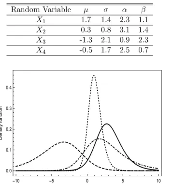
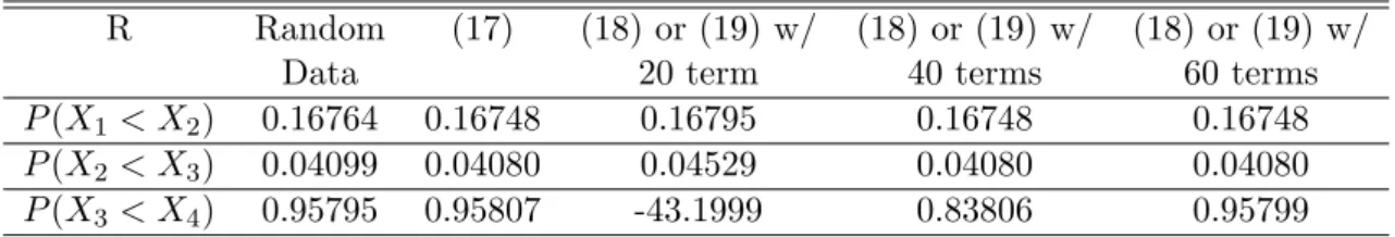
The present paper provides both the exact and approximated formulas for evaluating the reliability measureRwhen two generalized logistic distributions are considered. A set of four generalized logistic random variables is considered to show the applicability of (17), (18)and (19). Such variables are shown in Table 1 and graphically in Figure 1. Using the generalized logistic variables considered in Table 1, the reliability measures are obtained numerically by means of a computational code in Mathematica and given in Table 2.

Table 1: Logistic Random Variables Considered

Random Variable µ σ α β

X1 1.7 1.4 2.3 1.1

X2 0.3 0.8 3.1 1.4

X3 -1.3 2.1 0.9 2.3

X4 -0.5 1.7 2.5 0.7

-10 -5 0 5 10

0.0 0.1 0.2 0.3 0.4

x

Density

function

Figure 1: Probability Density Functions of the Random Variables from Table 1 (X1full,X2dotted, X3 dashed andX4dot-dashed).

The values of R estimated from random data have been obtained by the procedure below:

• For the random variablesXandY generate random samples with 105elements each,

Table 2: Reliability Measures

R Random (17) (18) or (19) w/ (18) or (19) w/ (18) or (19) w/

Data 20 term 40 terms 60 terms

P(X1< X2) 0.16764 0.16748 0.16795 0.16748 0.16748

P(X2< X3) 0.04099 0.04080 0.04529 0.04080 0.04080

P(X3< X4) 0.95795 0.95807 -43.1999 0.83806 0.95799

• Consider the indicator function I(x, y) = 1−u(x−y), where u(x) = 0,x < 0 and

u(x) = 1, otherwise. The value ofR is estimated by Re =

105

P

i=1

I(xi, yi);

• Repeat the above process 1000 times and then take the mean value of the Res

generated. These values are shown in Table 2.

It is worth noticing that the variance of the estimator used above was of order 10−7for all the cases. As can be seen from the analysis of Table 2, both the exact and approximate expressions obtained in the present paper correctly model the random data generated. Depending on the parameters of the distribution, the series presented may be slowly convergent. On the other hand, as the series themselves are quite simple to implement, taking more than 60 terms is not a hard task for any commercial computational software.

6. Conclusions

Skewness is present in most of the random data collected from nature. Even though mathematically simple, generalized logistic models have shown to be useful tools to model skewed data. The probability density and the cummulative distribution functions of the linear combination of N independent and not identically distributed generalized logistic random variables have been obtained in terms of the H-function.

The c.d.f. of the linear combination can be used to build reliability measures of the

typeP(

N1

P

i=1

Xi < N2

P

j=1

Yj) whenXi,i= 1, ..., N1 andYj,j = 1, ..., N2 are generalized logistic

random variables of type IV with different location, scale and shape parameters. Besides, a series expansion alternative expression has been derived for the caseN1 =N2 = 1.

The applicability of the expressions developed has been illustrated by numerical exper-iments, indicating a very good accordance between the exact and the estimated reliability measures.

Acknowledgements

References

[1] M. R. Alkasasbeh and M. Z. Raqab. Estimation of the generalized logistic distribution parameters: Comparative study. Statistical Methodology, 6(3):262–279, 2009.

[2] A. Asgharzadeh, R. Valiollahi, and M. Z. Raqab. Estimation of the stress-strength reliability for the generalized logistic distribution. Statistical Methodology, 15:73–94, 2013.

[3] N. Balakrishnan. Approximate maximum likelihood estimation for a generalized lo-gistic distribution.Journal of Statistical Planning and Inference, 26(2):221–236, 1990.

[4] P. K. Bhunya, R. D. Singh, R. Berndtsson, and S. N. Panda. Flood analysis using generalized logistic models in partial duration series. Journal of Hydrology, 420-421:59–71, 2012.

[5] A. Chaturvedi, S. Kang, and Pathak A. Estimation and testing procedures for the reliability functions of generalized half logistic distribution. Journal of the Korean Statistical Society, 45(2):314–328, 2016.

[6] B. M. Das and K. Sobhan.Principles of Geotechnical Engineering. Cengage Learning, Stamford, US, 8th edition, 2014.

[7] A. I. Gen¸c. Estimation ofp(x > y) with topp-leone distribution. Journal of Statistical Computation and Simulation, 83(2):326–339, 2013.

[8] R. Jacobs, A. A. Bekker, H. van der Voet, and C. J. Ter Braak. Parametric estimation of p(x ¿ y) for normal distributions in the context of probabilistic environmental risk assessment. PeerJ, 3:e1164, 2015.

[9] R. A. Johnson. Stress-strength model for reliability. In P. R. Krishnaiah and Rao C. R., editors, Handbook of Statistics, pages 27–54. Elsevier, Amsterdam, Netherlands, 1988.

[10] S. Kotz, S. Lumelskii, and M. Pensky. The Stress −Strength Model and its General-izations: Theory and Applications. World Scientific, Singapore, 2003.

[11] A. M. Mathai, R. K. Saxena, and Haubold H. J. The H-function: Theory and Appli-cations. Springer, New York (NY), 2010.

[12] M. M. Nassar and A. Elmasry. A study of generalized logistic distributions. Journal of the Egyptian Mathematical Society, 20:126–133, 2012.

[13] L. C. S. M. Ozelim, A. L. B. Cavalcante, A. P. Assis, and L. F. M. Ribeiro. Analytical slope stability analysis based on statistical characterization of soil primary properties.

[14] A. Ragab. Estimation and predictive density for the generalized logistic distribution.

Microelectronics Reliability, 31(1):91–95, 1991.

[15] Nadarajah S. and Kotz S. Linear combinations, products and ratios of t random variables. Allgemeines Statistisches Archiv, 89(3):263–280, 2005.

[16] H. M. Samawi, A. Helu, H. D. Rochani, J. Yina, and D. Lindera. Estimation ofp(x > y) when x and y are dependent random variables using different bivariate sampling schemes. Communications for Statistical Applications and Methods, 23(5):385–397, 2016.

[17] M. D. Springer. The Algebra of Random Variables. Wiley, New York (NY), 1979.

[18] L. Ventura and W. Racugno. Recent advances on Bayesian inference for p(x < y).

Bayesian Analysis, 6(3):411–428, 2011.