An Algorithm for Finding Two Node-Disjoint Paths in Arbitrary Graphs

Mehmet Hakan Karaata

Department of Computer Engineering, Kuwait University, Safat, Kuwait

An Algorithm for Finding Two

Node-Disjoint Paths in Arbitrary

Graphs

Given two distinct vertices (nodes) source s and target t of a graph G = (V, E), the two node-disjoint paths problem is to identify two node-disjoint paths between s V and tV. Two paths are node-disjoint if they have no common intermediate vertices. In this paper, we present an algorithm with O(m)-time complexity for finding two node-disjoint paths between s and t in arbitrary graphs where m is the number of edges. The proposed algorithm has a wide range of applications in ensuring reliability and security of sensor, mobile and fixed communication networks.

ACM CCS (2012) Classification: Networks → Net-work algorithms → Data path algorithms

Mathematics of computing → Discrete mathematics

→ Graph theory → Paths and connectivity problems

Keywords: disjoint paths, distributed systems, fault tolerance, network routing, security

1. Introduction

Given two distinct vertices (nodes) s and t of a graph G = (V, E) with set of vertices V and set of edges E, paths P1 _{and P}2 _{from vertex s to} ver-tex t are said to be node-disjoint iff paths P1 _and

P2 _{do not contain any common vertices except} for the endpoints.

The two node-disjoint paths problem is to find two node-disjoint paths from source vertex s to target vertex t [2]. The two node-disjoint paths problem is a fundamental problem with abun-dant number of applications in diverse areas including VLSI layout [3], [4], [5], reliable net-work routing [6], secure message transmission

[7], [2], and network survivability [8]. For in-stance, perfectly secure transmission can be im-plemented using node disjoint paths by breaking up data into several shares and sending them along the disjoint paths. This simple expedient makes it difficult for an adversary with bounded eavesdropping capability to intercept a trans-mission or tamper with it. In addition, the same crucial message can be sent over multiple dis-joint paths in networks that are prone to message losses to avoid omission failures or, in the pres-ence of faults, information on re-routing of traf-fic along the network can be provided. Recently, [8] introduced a new strategy for using network coding over p-Cycles to provide 1 + N protec-tion against single link failures in optical hyper-cube networks. Protection paths and cycles are commonly used in optical networks to enhance performance and reliability [9], [10], [11], [12]. The two node-disjoint path problem and its vari-ations are fundamental and extensively studied in graph theory. Algorithms to find edge-disjoint paths were proposed in [13], [14], [15], [16], [17], [3]. Ford and Fulkerson [18] proposed an

Fi-bonacci heaps) where n is the number of nodes in the graph. These algorithms involve calls to a regular shortest path algorithm; however, they require different graph transformations (e.g., re-moving links, changing link metrics) to ensure that the pair of edge-disjoint paths between a source and destination with the minimum sum of the metrics on the two paths is obtained (as-suming that at least one pair of disjoint paths exists). The graph transformations of Bhandari algorithm may generate links with negative metrics, as a result, it requires an associated shortest path algorithm such as BFS to handle graphs with negative link metrics. The run-times of Suurballe and Bhandari algorithms are about the same; however, the latter may be more read-ily extensible to other applications [20]. For that purpose, each node on the initial shortest path between the source and the destination is split into two nodes and another graph is constructed by a graph transformation process satisfying a number of properties.

Itai and Rodeh [21] presented an algorithm to compute two spanning trees of an undirected graph G rooted at s such that for any node v the two tree paths from s to v are edge-disjoint. If G

is 2-node connected then the two paths are also node-disjoint. The algorithm of Itai and Rodeh computes the two spanning trees via an s – t

numbering [22].

Another sequential solution to the problem of finding two disjoint paths between two end-points in arbitrary graphs is presented in [23]. This solution is based on identifying kernels using fundamental cycles in the graph. The first distributed algorithm for finding two node-dis-joint paths in arbitrary graphs based on the same idea of identifying kernels using fundamental cycles of Ishida et al. [23] is given in [24]. In addition, sequential solutions to the problem based on network flow also exists [17].

A distributed synchronous and asynchronous algorithm for disjoint paths is proposed in [25] for message passing system model. This algo-rithm makes use of some ideas from [19], [13] and reduced [19] approach into the problem of finding minimal shortest path instead of aug-mented path.

Our proposed algorithm has O(m)-time com-plexity whereas Suurballe-Tarjan and Bhandari algorithms have O(m + nlogn)-time complexity

while guaranteeing some properties about the paths found. The algorithm by Itai and Rodeh [21] can also be used to solve the disjoint paths problem with the same time complexity as ours. On the other hand, our algorithm has a very sim-ple basis given as a simsim-ple lemma and adopts an entirely different approach. The node disjoint paths algorithms based on Maximum-Flow computation such as Ford-Fulkerson and Suur-balle-Tarjan [19], [13] involve a number of phases after the discovery of a shortest path be-tween two endpoints. First, the initial graph is transformed into a new graph where arc weights and directions are recomputed. Second, each node on the shortest path is split and addition-al arcs are introduced leading to a new graph. Third, another shortest path is constructed be-tween the two endpoints in the newly obtained graph. Fourth, paths common between the two constructed disjoint paths and the cycles that do not contain both the endpoints are removed prior to constructing the two disjoint paths. On the other hand, the proposed algorithm is not Maximum-Flow computation based and the ba-sis of the algorithm is given in the form of a single lemma. It requires only the identification of link paths prior to the construction of the dis-joint paths. Therefore, the proposed algorithm is simpler and more understandable than those based on Maximum-Flow computation. In ad-dition, most solutions available in the literature [23], [24], [19], [13] suffer from being overly complex or being unfit for use in distributed applications. These drawbacks primarily stem from the adaptation of solutions to other fun-damental problems such as edge-disjoint paths, fundamental cycles (and kernel) and network flow to the solution of the node-disjoint paths problem. In addition, many of these solutions require the discovery of some global properties of the entire graph instead of local properties. These impose severe restrictions to the adapta-tion of the soluadapta-tions to distributed applicaadapta-tions. Therefore, it is not clear how these solutions could be used to devise a distributed solution to the node-to-node disjoint paths problem.

In this paper, we present a novel O(m)-time sequential algorithm for finding two node-dis-joint paths between two distinct vertices s and

P_i₁, 1 i k, is referred to as the

prede-cessor of P_i.

(iii) For each i, 1 ik, vertex o_i on P is select-ed to maximize d_s(w_i).

(iv) The terminus of the last link path P_k is tar-get wk = t.

P(v, w) denotes the subpath of P with origin v

and terminus w. P(v, w], P[v, w), and P[v, w] denote the same path excluding the terminus, origin, and both the origin and the terminus of the subpath P(v, w), respectively. Let P₁, P₂, ...,

P_k be a sequence of link paths in G for a shortest path P between s and t. Also, let o_i and w_i for 0  ik denote the origin and the terminus of link path P_i. Let P′ = P₁ P[w₁, o₃] P₃P[w₃, o₅]

P₅...P_2l+1 where 2l + 1 k and 2(l + 1) + 1 k, and P″ = P(s, o₂) P₂ P[w₂, o₄] P₄...P_2l where 2lk and 2(l + 1) k be two paths in G. Using the above definitions, we define paths P1 _and

P2 _{as follows. If k is odd, P}1 _{= P′ and P}2 _{= P″}

P[w_k1, t). Otherwise, P1 _{= P′ P[w}

k1, t) and

P2 _{= P″.}

The following lemma establishes the basis of the proposed algorithm.

Lemma 1. Let P be an arbitrary path between two arbitrary but distinct vertices s and t in

G = (V, E). Graph G contains two node-disjoint paths P1 _{and P}2 _{between endpoints s and t iff} there exists a maximal sequence of link paths

P₁, P₂, ..., P_k in G for P satisfying the four con-ditions for being a sequence of link paths.

Proof. For the ''if'' direction, we prove the con-trapositive. We assume that the sequence of link paths LP = P₁, P₂, ..., P_k does not exist and we show that two disjoint paths do not exist. Ob-serve that the sequence LP = P₁, P₂, ..., P_k does not exist if at least one of link paths P_i i k

does not exist. First, if the link path P₁ does not exist, then the successor of s on P is common for all the paths starting from s. Now, consider the case where link paths P₁, P₂, ..., P_i, 1 ik, exist and the next link path P_i+1 does not ex-ist. Analogously to the above, the terminus of

P_i is common for all the paths starting from s. Thus, in both cases, two disjoint paths between

s and t cannot exist, hence, the result. For the ''only if'' direction, we prove by construction. We assume that if the sequence of link paths

LP = P₁, P₂, ..., P_k exists, then two disjoint graphs given as a single lemma in the paper. In

addition, the proposed algorithm is designed in a way to ease its transformation to a distributed implementation. As a result, the proposed ap-proach is well suited for devising distributed and fault-tolerant solutions to the problem. It is anticipated that this work will initiate further work in the area of distributed and fault tolerant computing.

The paper is organized as follows. Section 2 presents the basis of the algorithm and some required notations for the formal description of the algorithm. Section 3 presents the two node-disjoint paths algorithm. In Section 4, we provide a correctness proof and the proofs of the time complexity bound of the algorithm. We conclude the paper in Section 5 with some final remarks.

2. Basis of Algorithm

In this section, we present the basis of the pro-posed solution. Let G = (V, E) be a graph with two distinct vertices s, t  V such that G con-tains two node-disjoint paths between s and t. We first define link paths to facilitate the de-scription of the basis of the algorithm.

Definition 1. Let P be a path between s and t

and d_s(v) the distance of vertex v on P from ver-tex s. A link path of path P in G is a path disjoint from P except for its endpoints that extend from a vertex o on P to a vertex w on P such that w

is the farthest vertex reachable from o, i.e., the distance from o to w is maximal. A vertex is said to be reachable from another vertex if the graph contains a path connecting them.

Let us now define LP = P₁, P₂, ..., P_k to be a maximal sequence of link paths of path P in G, each of which has its endpoints on P such that the following four conditions are satisfied by LP. (i) P₁ is the first link path with origin o₁(= s)

and terminus w₁.

(ii) Each link path P_i₁ where 1 i  k has a

successor link path P_i that extends from its origin o_i to its terminus w_i such that

1 2 1

2 1

( ) ( ) ( ) ( 2)

( ) ( ) ( ) if 2

s s s

s i s i s i

d o d o d w i

d w_ d o d w_ i k

  



 _{   }



paths P1 _{and P}2 _{exist and can be constructed as} follows:

(i) if k is even (k = 2l), then P1 _{= P}

1, P(w1, o3),

P₃, P(w₃, o₅), ..., P_2i+1, P(w_2i+1, o_2i+3), ...,

P_2l1, P(w_2l1, w_2l = t] and P₂ = P[o₁ = s, o₂),

P₂, P(w₂, o₄), P₄, ..., P(w_2i, o_2i+2), P_2i+2, ...,

P(w_2l₂, o2l), P2l (see Figure 1);

(ii) otherwise, i.e., k is odd (k = 2l + 1), then

P1 _{= P}

1, P(w1, o3), P3, P(w3, o5), P5, ...,

P(w_{2i + 1}, o_{2i + 3}), P_2i+3, ..., P(w_2l1, o_{2l + 1}),

P_{2l + 1} and P2 _{= P[o}

1 = s, o2), P2, P(w2, o4),

P₄, P(w₄, o₆), ..., P_2i, P(w_2i, o_{2i + 2}), ..., P_2l;

P(w_2l, w_2l+1 = t]. _□

The proposed algorithm constructs the two node-disjoint paths between s V and t V in four phases executed in sequence, namely the

forest construction, the discovery of the farthest reachable vertex on the shortest path, the con-struction of link-paths, and the node-disjoint paths construction phases.

We assume that a shortest path P from s to t has been constructed. In the first phase, a spanning forest is constructed, where each tree in the for-est is rooted at a vertex on P with certain prop-erties. The constructed forest is used to find, for each vertex v on P, the farthest vertex w on

P reachable via path P_v disjoint from P and to discover path P_v from v to w. Then, in the sec-ond phase, for each vertex v on P, the farthest vertex on P reachable from v via a path disjoint from P is discovered. Subsequently, in the third phase, link paths P₁, P₂, ..., P_k are identified as follows. First, link path P₁ is identified as a path originating at s(= o₁) with terminus w₁ such that

P₁ is disjoint from P (except for its endpoints) and w₁ is the farthest reachable such vertex on path P. Second, link path P₂ is identified as a path disjoint from P (except for its endpoints) originating at vertex o₂ on subpath P[s, w₁] of

P and terminating at vertex w₂ on P such that

d_s(w₂) is maximal. Third, link path P₃ is iden-tified as a path disjoint from P (except for its endpoints) originating at vertex o₃ on subpath

P[w₁, w₂] of P and terminating at vertex w₃ on

P such that d_s(w₃) is maximal. In the same man-ner, P₄ is identified with its origin on subpath

P[w₂, w₃] of P with its terminus w₄ on P such that d_s(w₄) is maximal, and so on. Then, in the fourth phase, two node-disjoint paths P1 _{and P}2 are identified using the link paths P₁, P₂, ..., P_k

and shortest path P as follows. The maximal

sequence of link paths with odd subscripts P₁,

P₃, ..., P_2l+1 where 2l + 1 = k or P₁, P₃, ..., P_2l1

where 2l = k (depending on whether k is odd or even) are used to construct path P1_{, whereas} the maximal sequence of link paths with even subscripts P₂, P₄, ..., P_2l where 2l k are used to construct P2_{. In each sequence, for every pair} of consecutive paths in the sequence, such as P₁

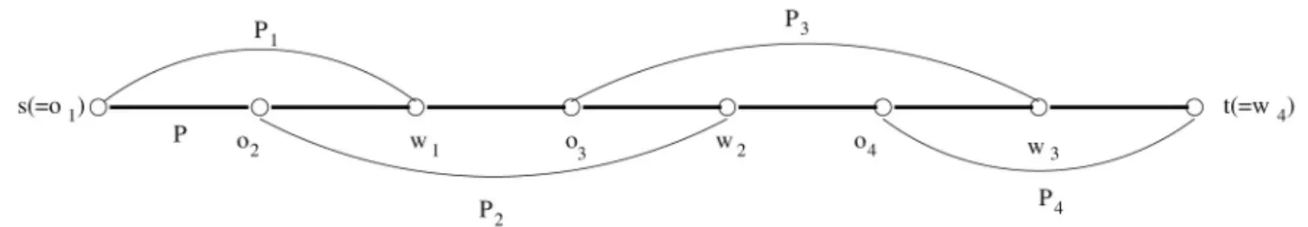
and P₃ in the sequence of odd subscripted link paths, the terminus of each link path and the ori-gin of the subsequent link path are connected by a segment of P between the terminus of the first link path of the pair and the origin of the subse-quent link path on P to construct a disjoint path. Figure 1 depicts a graph with source vertex s, target vertex t and its link paths P₁, P₂, P₃ and

P₄ for shortest path P (shown by a thick line) from s to t to illustrate the above approach. Note that, although not shown, we assume that each of the link paths P₁, P₂, P₃ and P₄ con-tain multiple vertices on them other than their endpoints to make P a shortest path in G. Ob-serve that link path P₂ is a successor of link path P₁, P₃ is a successor link path of P₂, and so on. Figure 2 shows the same graph shown in Figure 1 with the node-disjoint paths P₁ and

P₂ identified to illustrate the approach to con-struct the node-disjoint paths. Observe that the figure depicts node-disjoint path P₁ shown with thicker lines and P₂ shown with thick lines. No-tice that the odd subscripted link paths P₁ and

P₃ are used to construct node-disjoint path P1_, whereas, the even subscripted link paths P₂ and

P₄ are used to construct node-disjoint path P2_. Also notice that subpaths P[w₁, o₃] and P[w₃, t) of P are added to the link paths P₁ and P₃ to construct P1_{. Similarly, subpaths P(s, o}

2] and

P[w₂, o₄] of P are added to the link paths P₂ and

P₄ to construct P2_.

3. Algorithm

In this section, we provide a formal description of the algorithm to find two disjoint paths. Let G = (V, E) be a simple undirected graph with two distinct vertices s, tV such that two node-disjoint paths exist between s and t. Let

P = (V_P, E_P ) be a shortest path in G from s

available in the literature, such as [26]. We also assume that for each vertex v on P, the d_s -val-ue d_s(v) of vertex v denoting its distance from source vertex s is also computed and available to our algorithm. We present our proposed algo-rithm in the next four subsections, where each subsection contains part of the algorithm imple-menting a phase of the algorithm.

3.1. Forest Construction

In the first phase of the algorithm, for each ver-tex r on P, a maximal BFS tree T_r = (V_T, E_T) called linktree rooted at r is constructed in G. The tree T_r satisfies that each vertex w in G is a descendant of r in T_r iff w is reachable from

r through a path in G not on P and d_s(r) is min-imum. That is, each vertex w in G is a descen-dant of root r on P iff it is reachable from r via a path in G not on P such that r is the root among all such roots on P that makes d_s(r) minimum. Forest F is defined as the set of all link trees rooted at nodes on P.

Prior to presenting the algorithm to construct forest F, we need the following definitions. Variables V_T and E_T denote a set of vertices and edges included in forest F constructed thus far, respectively. Variable Q denotes a queue of vertices that have not been visited yet. Variable

m(v) for each vertex vV denotes whether or not vertex v has been visited in the process of constructing F. Variable p(v) for each vertex

v  V denotes the parent of vertex v. Ordered set P = s, v₁, v₂, ..., v_k, t denotes a shortest path in

G from vertex s to vertex t. Statement for each

v P  in order executes its body for each value v assigned in order from ordered set P. If phrase in reverse order is used instead of in order, the body is executed for each element of the ordered set P in reverse order. A variation of the statement for eachvP | predicate

ensures that the body is executed for those v

that satisfy predicate  predicate . Variable

pred(v) denotes the predecessor of vertex v on

P. The algorithm requires the following input parameters: set of vertices V, set of edges E in

G, and an ordered set of vertices of a shortest path P between s and t.

The implementation of the first phase of the al-gorithm to construct a maximal BFS forest F

of G with the aforementioned property is given with Algorithm 1.

3.2. Discovery of the Farthest Reachable Vertex on the Shortest Path

The objective of the second phase is to allow each vertex r on P to discover the d_s-value of the terminus vertex w with the largest d_s-value (if it exists) of potential link paths originating at r. A potential link path is a path in G disjoint from P except for its endpoints which are on P. To implement the objective of the second phase, each vertex v in V_T maintains a variable l(v) that stores the maximal d_s-value among reachable vertices on P from v through a potential link path if it has such a reachable vertex(vertices), and 0 otherwise. This is implemented as

fol-Figure 1. A graph with its link paths identified for source s and target t.

lows. First, for each vertex in V_T , the l-value of each vertex is assigned 0. After that, in a bottom up manner, starting from leaves, each vertex computes its l-value as the maximum of

l-values of its children in V_T and its neighbors'

d_s-value on P. When the l-value is computed for a vertex v, it discovers the farthest reachable vertex on P from v through a segment of link path originating at vertex r on P (as l(v) rep-resents the d_s-value of such vertex on P). The computation of the l-values in T_r marks link paths originating at r as maximal paths with or-igin r on the vertices whose l-values are equal to l(r). Algorithm 2 provides an implementation of the second phase of the algorithm.

Thus far, we presented the first two phases of the algorithm where each vertex r on P dis-covers the d_s-value of the farthest vertex on P

reachable from r via a link path. In addition, each vertex r on P marks the link path origi-nating at r. These link paths (or subset of them) will be used to construct the two disjoint paths in the later phases.

3.3. Identification of Link Paths

We now present the third phase of the algorithm to identify origins and terminuses of all link paths in LP = P₁, P₂, ...,P_k using information collected in the previous two phases. For that purpose, first, vertex s = o₁ is identified as the origin of the first link path P₁. We know that l(s) contains the d_s-value of the farthest vertex from

s on P reachable via a link path. The vertex with

d_s-value equal to l(s) is identified as the termi-nus w₁ of P₁. Then, in order to find the origin of P₂, the vertex with the largest l-value in the interval [s, w₁] is identified as the origin o₂ of

P₂. Observe that l(o₂) contains the d_s-value of the farthest vertex from o₂ reachable via a link path which is the terminus w₂ of P₂. Then, for each link path P_i, 2 ik, the origin o_i of link path P_i is identified as the vertex with the larg-est l-value on P[w_i₂, w_i₁], while the terminus w_i of P_i is identified as the vertex whose d_s -val-ue is equal to l(o_i). For example, origin o₃ of P₃

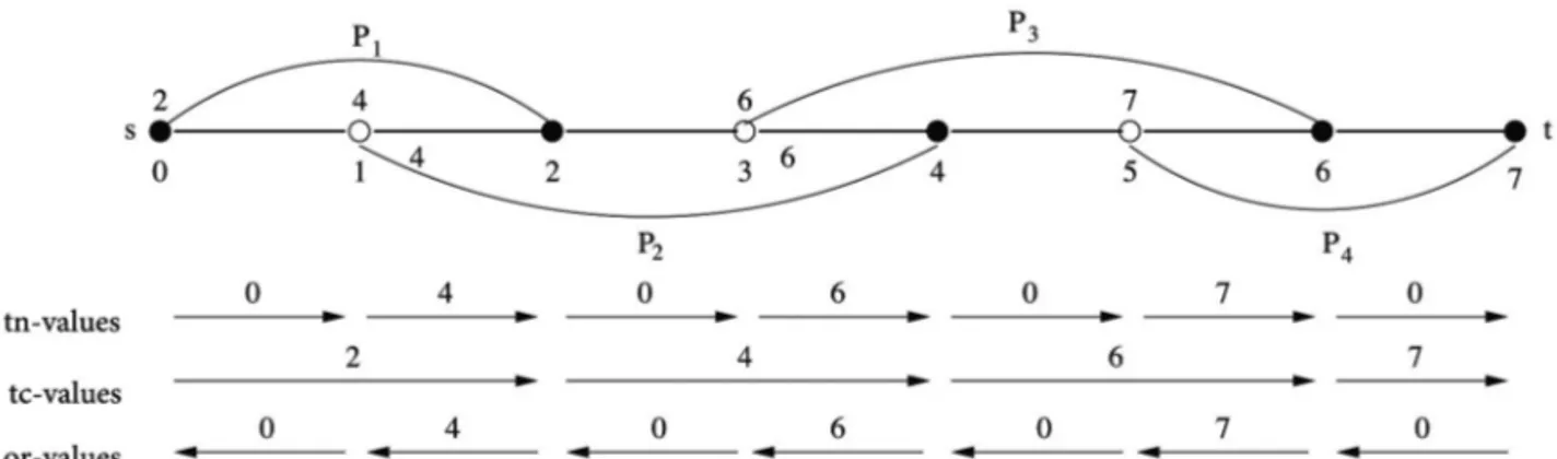
is the vertex that has the largest l-value among vertices on P[w₁, w₂] and terminus w₃ of P₃ is the vertex whose d_s-value is equal to l(o₃). Figure 3 illustrates the approach adopted by the third phase of the algorithm. In the figure, the

numbers above the vertices denote the d_s -val-ues, whereas the numbers below the vertices denote the l-values of the corresponding verti-ces. Since the l-value of s is 2, P₁ extends from

s to w₁. The origin of P₂ is o₂ since o₂ has the largest l-value of 4 among vertices on P[0, 2]. Similarly, since o₃ has the largest l-value of 6 among the vertices on P[2, 4], the origin of P₃ is

o₃, and so on. We now describe the implementa-tion details of the above approach. For each ver-tex v V_T , three integer variables tc(v), tn(v), and or(v) are maintained by the algorithm. The two variables tc(v) and tn(v) are used to hold the d_s-value of current and next terminuses, re-spectively, of link paths as the vertices on P are traversed starting from s towards t.

For each i, 1 ik, tn-values are used to find the largest l-value encountered thus far among ver-tices on P[w_i1, w_i] (or from the origin of P₁ to its terminus for i = 2) towards t on P. Whereas,

tc-values are used to propagate the largest l -val-ue found between w_i1 and w_i on P (using tn -val-ues), from terminus w_i to terminus w_i+1 on P. The reason for using two variables to find and propagate the largest l-value from the origin of a link path to its terminus is as follows. Ob-serve that for i, 1 ik, we need to separately propagate the largest l-value on P[w_i, w_i+1] that was found on P[w_i1, w_i] and find the largest

l-value found so far on P[w_i, w_i+1]. Propagat-ing the first value is necessary for identifyPropagat-ing

w_i+1

,

while finding the second value is required for identifying w_i+2. Since the propagating and finding the values takes place on the same in-terval and they depend on each other, the dis-covery and the propagation on both cannot be implemented using a single integer variable. Therefore, we use two variables, namely tn and

tc for each vertex to implement the discovery and the propagation of the largest l-values. The tc and tn-values are computed in the follow-ing manner. The tn-value of node s and upon its discovery, tn-value of the terminus w_i of each link path P_i, 1  i k, is assigned 0. Then, ev-ery other vertex assigns to its tn-value the larg-est of its predecessor's tn-value and its l-value. Upon completion of these assignments, for each

i, 1  i  k, tn(pred(w_i), where w_i is the termi-nus of link path P_i, contains the largest l-value among vertices on P[w_i1, w_i] (or P[s, w₁] for

Algorithm 1. Forest construction.

1. procedure TWODISJOINTPATHALGORITHM(V, E, P) 2. booleanm(v) :false for each vertexvV ;

3. vertexIdp(v) for each vertexvV ; 4. vertexSetV_T;

5. edgeSet E_T; 6. queue Q;

7. for all vP in order do 8. V_T :V_T ∩ {v}; 9. m(v) :true; 10. addQueue(Q, v); 11. whileempty(Q) do 12. xremQueue(Q);

13. if {xP→d_s(x) d_s(v) = 1} then 14. pred(x) v;

15. end if

16. for allwV \ P|{x, w} E {x, w} E_Tm(x) m(w) do 17. addQueue(Q, w);

18. m(w) true; 19. p(w) x; 20. V_T :V_T ∩ {w}; 21. E_T :E_T ∩ {x, w}; 22. end for

23. end while 24. end for 25. end procedure

Algorithm 2. Discovery of the farthest reachable vertex on the shortest path.

1. integer l(v) for each vertex vV_T ;

2. m(v) :false; l(v)  0; for each vertexvV_T ;

3. for allvV_T |m(v) {v, w} E_T {(p(w) v→m(w)} do

4. l(v) :max{max_{{v, z} E}

Tz P{v, w P→ds(w) ds(v) 1}{ds(z)},

5. max_{{v, z} ETp(z) vzP} {l(z)}, 0}; 6. m(v) true;

7. end for

P_i, 1 i k, the largest l-value among vertices on subpath P[w_i2, w_i1] kept in tn(pred(w_i1)) needs to be propagated towards t up to the vertex whose d_s-value is equal to tn(pred(w_i1)) so that this vertex is identified as the terminus of P_i+1. This is implemented using the tc-value comput-ed at the same time with tn-value for each vertex as follows. The l-value of s is assigned to tc(s) and upon its discovery, the terminus w_i of each link path P_i, 1  i  k, assigns tn(pred(w_i)) to

tc(w_i). Then, each of the consecutive vertices as-signs its tc-value, the tc-value of its predecessor in P. This propagation continues until encoun-tering the (terminus) vertex whose d_s-value is equal to the propagated value. That is, each ter-minus w_i, 1 ik, of a link path is discovered by node w_i on P upon discovering that d_s(w_i) = tc(pred(w_i)) holds. When tn and tc-values of all the vertices on P are computed, each ver-tex whose d_s and its predecessor's tc-values are equal is identified as a terminus vertex of a link path. In this manner, the tc and tn-values of the vertices on P are computed in order, and the ter-minuses of the link paths in LP are identified one after the other.

We now describe how variable or(v) is used to identify origins of link paths. Upon discovering all terminuses of link paths, observe that pre-decessor of w_i stores in tn(pred(w_i)) the largest

l-value found in the interval [w_i2, w_i1], for 2 ik. In order to find origin o_i, tn(pred(w_i)) is assigned to or(pred(w_i)) and the or-value is propagated toward s until meeting a vertex on

P with l-value equal to the propagated or-value. This vertex is identified as the origin o_i of P_i. This procedure is applied to all vertices on P

starting from t until reaching s and identifying the origins of link paths.

Next, we describe the details of identifying the origins of link paths. After all tc and tn-values of vertices on P are computed (and the identification of the terminuses of the link paths), or-values of vertices on P are computed in reverse order of vertices in P as follows. First, or(t) is assigned 0. In reverse order of vertices in P[w_k1, w_k], each vertex assigns 0 to its or-value when it copies its successor's or-value. In this process, upon identifying itself as a terminus vertex by discovering that tn(w_k1) = 0, vertex w_k1 as-signs tn(pred(w_k1)) to or(w_k1). Then, the value in or(w_k1) is propagated towards vertex s in re-verse order of vertices as vertices in ordered set

P(w_k2, w_k1) copy the or-value of their succes-sors to their or-values. The propagation of the value continues until vertex o_k on P[w_k2, w_k1] such that l(o_k) = or(o_k) holds. Observe that the vertex on subpath P[w_i2, w_i1] with the largest

l-value is the origin o_i of link path P_i. In order for vertex o_i, 1 ik, to discover that it is the origin of P_i, the tn-value of pred(w_i1) contain-ing the largest l-value on P[w_i2, w_i1] needs to be propagated towards s until the vertex whose

l-value is equal to tc(pred(w_i1)) is encountered using the or-values. For that purpose, first, the largest l-value on subpath P[w_i1, w_i] stored in

tn(pred(w_i)) is assigned to or(w_i). Subsequently, this value is propagated using the or-values of vertices on subpath P(o_i, w_i1) towards s until the vertex o_i with l-value is equal to the prop-agated value. Then, vertex o_i whose or-value is equal to its l-value is identified as the origin of link path P_i. The above approach is imple-mented through the following actions. For each vertex v on P in reverse order, if v = pred(w_i),

i.e., v is the predecessor of terminus w_i of a link path P_i, for 1  i  k, the value tn(pred(w_i)) is assigned to or(w_i), if v = pred(o_i), i.e., v is the predecessor of origin o_i of link path P_i, zero is assigned to or(v), and otherwise, or(suc(v)) is assigned to or(v).

Figure 4 illustrates the usage of tn and tc -val-ues for the propagation of the l-values and the discovery of terminuses of link paths. In Figure 4, the numbers below the vertices denote the

d_s-values of the vertices, whereas, the numbers above the vertices denote the l-values of the vertices. Vertices s, t, and those that are termi-nuses of link paths are denoted by filled circles to indicate the vertices whose tn-values are 0. Each row of arrows in the figure denotes the propagation of values using variables tc, tn, or

or-value direction in which the computation of a variable is carried out. The top row of arrows in the figure illustrates the computation of the

tn-values, whereas the second and the third rows of arrows illustrate the computation of the tc and

or-values, respectively, of the vertices on P. The number above each arrow denotes the values as-signed to tc, tn, or or-values of the vertices in the subpath of P above the arrows. As shown by the arrows, l-value of s propagates towards

t until the vertex whose d_s-value is 2 using the

d_s-value 1 to the one with d_s-value 2, they cannot be used to propagate 4. Therefore, tn-values are used to carry 4 until the vertex with d_s-value 4. The tn-value of s, the origin of P₁, is set to 0 and

tn-values are computed towards t incrementally to collect the largest l-value on P encountered so far until the terminus w₁ of P₁, the vertex whose d_s-value is 2 in the figure. Upon com-pletion of this, tn(w₁) is set to 0 and the tn-value of the predecessor of w₁ (pred(w₁)) contains the largest l-value on P(s, w₁]. Then, the tn-value of

pred(w₁) is assigned to the tc-value of w₁ and this value is propagated using tc-values over the subpath P(w₁, w₂) until encountering ver-tex (w₂) whose ds-value is equal to propagated value to identify the terminus w₂ of P₂ in the aforementioned manner. While this propagation takes place, the largest l-value on P(w₁, w₂) is found using the tn-values. In this manner, the tn

and tc-values are computed and the terminuses of link paths are identified. However, the ori-gins of link paths are not yet explicitly identi-fied when the aforementioned computation is carried out starting at s and continuing towards

t. For that purpose, the or-values are computed as follows. First or(t) is assigned 0. Notice that in Figure 4, the vertex with d_s-value of 6 starts the propagation of value 7, and it continues until reaching the vertex with l-value of 7. Then, this vertex is identified as the origin of a link path. Similarly, the vertex with d_s-value of 4, starts the propagation of value 6, and it continues until reaching the vertex with l-value of 6. Then, this vertex is identified as the origin of a link path. Algorithm 3 shows the third phase of the algo-rithm implementing the above strategy. In the

description of the algorithm suc(v) refers to the successor of vertex v on P.

When the third phase of the algorithm termi-nates, the following propositions hold. As a re-sult, the origins and the terminuses of link paths are identified.

Proposition 1. Vertex vP is the terminus of a link path iff tc(pred(v)) = d_s(v) holds.

Proposition 2. Vertex v P is the origin of a link path iff l(v) or(v) holds.

Algorithm 3. Construction of link-paths.

1. integertc(v); tn(v), or(v) for each vertexvV ; 2. tc(s) :l(s);

3. tn(s) : 0;

4. for allvP\{s} in order do 5. ifd_s(v) tc(pred(v)) then 6. tc(v) :tc(pred(v));

7. tn(v) :max{tn(pred(v)); l(v)}; 8. else

9. tc(v) :tn(pred(v)); 10. tn(v) : 0;

11. end if 12. end for 13. or(t) : 0;

14. for allvP \ tin reverse order do 15. iftn(v)  0 then

16. if (l(suc(v)) = or(suc(v))) then 17. or(v) : 0;

18. else

19. or(v) :or(suc(v)); 20. end if

21. else

22. or(v) :tn(pred(v)); 23. end if

24. end for

3.4. Construction of Disjoint Paths

We now present the fourth phase of the algo-rithm that constructs the node-disjoint paths P1 and P2 _{based on the previous three phases.} Using the link paths and the shortest path P, node-disjoint paths P1 _{and P}2 _{are constructed as} follows. First, the first vertex on each is deter-mined to be s. Second, the second vertex on P1 is determined to be the neighbor of s on P₁, i.e., the second vertex on P1 _{is assumed to be the} neighbor of s with the largest l-value. In addi-tion, the second vertex on P2 _{is determined to be} the neighbor of vertex s on P. After determin-ing the first two vertices on P1 _{and P}2_{, disjoint} paths P1 _{and P}2 _{are extended in the same} man-ner, as follows. Let v be the last vertex on the disjoint path, either P1 _{or P}2_{, constructed thus} far. Notice that vertex v can either be a vertex on P or on a link path. We first consider the case where v is on path P. If l(v) or(v) holds for v

on path P, then the next vertex is determined to be the neighbor of v with the largest l-value,

i.e., the next vertex is the second vertex on the link path whose origin is v. Otherwise, the next vertex is the successor of v on P. We now con-sider the case where vertex v is on a link path. In this case, the next vertex is determined to be the next vertex on the link path. Recall that the successor of vertex v on a link path is a child of

v in T with the largest l-value. The construction of each disjoint-path ends after the target vertex

t is added to the path.

We need the following definitions to facilitate the description of the fourth phase of the al-gorithm. Function app(P, v) appends vertex v

at the end of path P. Function succ_P(v) returns the successor of vertex v on path P. Function

last(P) returns the last vertex on path P. N_v de-notes the neighboring vertices of vertex v in G.

4. Correctness

In this section, we present a number of lemmas to establish the correctness of the proposed al-gorithm.

Lemma 2. After the completion of the first phase of the algorithm, a tree T (V_T, E_T ) rooted at vertex s is constructed in G such that for each vertex v and w on P, if d_s(v)  d_s(w)  1, then

vertex v is the parent of vertex w, and for each vertex v on P, each vertex w in G′  (V \ P, E \ P_E) where P_E denotes the set of edges connecting consecutive vertices in P, reachable via a path in G′ from vertex v on P such that d_s(v) is mini-mal, is a descendant of v.

Proof. Observe that, in the first phase of the algorithm, vertices on P are added to T in or-der. Also observe that after each vertex v on P

is added, all the vertices in G reachable from v

via a path that does not contain a vertex on P

are added in a BFS manner. Hence, proof fol-lows. _□

Lemma 3. Upon completion of this phase,

l(v)-value of each vertex on P denotes the

d_s-value of the farthest vertex from s on P

reachable via a path disjoint from P (except for its endpoints.)

Proof. Observe that for each vertex v T, the second phase of the algorithm computes the largest d_s-value among vertices on P that are in-cident on a non-tree edge connecting these ver-tices on P to descendants of v in T and assigns it to its l-value, l(v) in a bottom-up manner in T. Hence, proof follows. _□

Lemma 4. Let LP  P₁, P₂, ..., P_k be a se-quence of link paths in G for source s, target t

and shortest path P between s and t. P₁ is a link path with origin s and terminus v(l(s)), where

v(l(s)) denotes the vertex on P with d_s -val-ue equal to l(s). P₂ is a link path with origin

o₂  v(max_l(s, v(l(s)))) and terminus v(l(o₂)), where max_l(v₁, v₂) denotes the largest l-value among vertices on the subpath of P that extends from v₁ to v₂ on P. For each link path Pi, 2 ik, the origin o_i of link path P_i is identified as the vertex with the largest l-value among vertices on P with the d_s-value on P(d_s(w_i2), d_s(w_i₁)),

where w_i2 is the terminus of link path P_i2 and

o_i₁ is the origin of link path P_i₁. Whereas the

terminus of each link path P_i, 0  i  k, with origin o_i is vertex v(l(o_i)).

Proof. Clearly the first link path P₁ originates at

s. Since l(s) denotes the d_s-value of the farthest reachable vertex from s on P reachable via a path disjoint from P, and by Lemma 3 and the definition of link paths, P₁ terminates at v(l(s)). Also by Lemma 3 and the definition of link paths P₂ is a link path extending from origin

Notice that for 1 ik, the origin o_i of P_i is the vertex with the largest l-value on P(o_i1, w_i₁).

Since the origin o_i+1 of P_i+1 needs to be on

P(o_i, w_i) but cannot be on P(o_i1, w_i), origin

o_i+1 is on P(w_i1, w_i). Inductively, by Lemma 3 and the above, it is easy to show that for each link path P_i, 2 ik, the origin o_i of link path

P_i is identified as the vertex with the largest

l-value among vertices on P with the d_s-value on P(d_s(w_i2), d_s(w_i1)), where w_i2 is the ter-minus of link path P_i2 and w_i1 is the terminus of link path P_i1, whereas the terminus of each link path P_i, 0  i  k, with origin o_i is vertex

v(l(o_i)). _□

Lemma 5. Upon completion of the third phase of the algorithm, each vertex of a link path dis-covers whether or not it is an origin or a termi-nus of a link path only using the variables of the vertex.

Proof. Let P_i, 0 ik, be a link path with ori-gin o_i and terminus w_i.

In the third phase of the algorithm, using the tn

and tc-values, the terminus of each link path P_i

starting from link path P₁, one after the other, is identified as follows. On path P₁, value l(s) is copied form a vertex to another towards t

us-ing tc-values, when the copied value is equal to the d_s-value of a vertex, this vertex is identified as the terminus of P₁. While value l(s) is cop-ied to vertex w₁, tn-values are used to find and copy the largest l-value on P[s, w₁]. This larg-est value is used to identify the terminus of P₂

in the same manner by copying the value start-ing from w₁ from a vertex to another towards t

using tc-values. For the subsequent link paths,

tn-values are used to find the largest l-value be-tween two consecutive terminuses w_i and w_i+1

and this value is copied form a vertex to anoth-er from the lattanoth-er tanoth-erminus w_i+1 towards t using

tc-values to discover terminus w_i+2. Upon dis-covery of each terminus, its tn-value is set to zero to start discovering the next largest l -val-ue between the terminus and the consecutive terminus. Based on these arguments, it is easy to inductively show that all terminuses of link paths are identified and their tn-values are set to zero upon completion of the third phase of the algorithm.

Now, we are to show whether or not a vertex is the origin of a link path using only the variables of the vertex. Notice that after the third phase of the algorithm is completed and the terminuses are identified, tn(s)  0 and tn(w_i)  0 hold for each P_i, 0 ik. Also notice that after the third

Algorithm 4. Node-disjoint paths construction.

1. pathP1, P2 :s;

2. app(P1, v), where vN_s|jN_s{l(v) l(j)};

3. app(P2, succ_P(s)); 4. complete-path(P1); 5. complete-path(P2); 6. terminate;

7. functioncomplete-path(Q); 8. whilelast(Q) tdo 9. if (last(Q) P) then

10. if (l(last(Q)) or(last(Q))) then

11. app(Q, v), wherevN_last(Q) | _jNlast(Q){l(v) l(j)}; 12. else

13. app(P2, succ_P(s)); 14. end if

15. else

16. app(Q, v), wherevN_last(Q)|last(Q) p(v) l(last(Q)) l(v); 17. end if

phase of the algorithm is completed, all the fol-lowings hold.

For every vertex v on P[o_i, w_i], tn(v) denotes the largest l-value among vertices on P[o_i, v]. For each terminus vertex w_i, 0 ik1, tn(pred(w_i)) denotes the largest l-value of vertices on

P[w_i

,

w_i+1] and the l-value of the vertex that is the origin of link path P_i+2. tn(pred(t)) denotes the largest l-value (if any) of a potential link path between w_k1 and w_k. Otherwise, i.e., if no potential link path exists between w_k1 and w_k,

tn(pred(t)) denotes 0.

For every i, 0 ik , or-values of all the vertices on path P[w_i, w_i+1] contain value tn(pred(w_i)) which is the l-value of the origin of P_i+2.

Therefore, for each i, 0 ik, or-values of all vertices on path P(w_i, w_i+1) denote the largest

l-value of vertices on P[w_i, w_i+1). Since the ori-gin of each link path P_i+2, 1 ik1 is the ver-tex with the largest l-value on path P[w_i, w_i+1], then vertex with the largest l-value on this path is the origin of a link path iff l(v) or(v). Hence, the proof follows. _□

Lemma 6. Paths P1 _{and P}2 _{constructed by the} algorithm are disjoint between s and t.

Proof. First observe that both P1 _{and P}2 _start at s and the second vertex on P1 _{is the second} vertex on P₁, whereas the second vertex on P2 _is the second vertex on P. Notice that these choic-es of the second verticchoic-es on both P1 _{and P}2 _are not necessarily unique, however, the choice made leads to the construction of disjoint paths. Now, we are to show that function call com-plete-path(P1_{) constructs P}1 _{by including all} odd numbered link paths, subpaths of P con-necting the terminus of one odd numbered link path to the origin of the consecutive odd numbered link path, and if the terminus of the last odd numbered link path is not t, the sub-path of P connecting the terminus of the last odd numbered link path and t. Clearly, func-tion complete-path(P1_{) in each step adds a new} vertex v to the constructed path whose last vertex is v′ that satisfies the following. If v′ is on P and v′ is not an origin of a link path, i.e., (tc(v′) or(v′)). If v is the next vertex on P, v′ is on a link path, v is the next vertex on the link path. Otherwise, if v′ is the origin of a link path, then v is the next node on the link path with v

as its origin.

Observe that this scheme ensures that after in-cluding an odd numbered link path in P1 _{and a} number of vertices towards t are added to P1 until encountering the next origin of a link path which happens to be the origin of the consec-utive odd numbered link path or t. This is be-cause the origin of the even numbered consec-utive link path precedes the odd numbered link path on P. It is easy to see that disjoint path P2 is constructed in an analogous manner. It is also easy to see that, since odd numbered and even numbered link paths are node-disjoint, afore-mentioned subpaths of P connecting odd num-bered and even numnum-bered subpaths are disjoint, and P(s, o₂) is included only in P2 _{and P(w}

k1, t) is included in one of the disjoint paths P1 _{or P}2_, paths P1 _{and P}2 _{are disjoint.}

□

Lemma 7. The proposed algorithm has time complexity of O(m).

Proof. It is easy to see that the first, the second, the third and the fourth phases of the algorithm have the time complexities of O(m), O(m),

O(D), and O(n), respectively, where D denotes the diameter of the graph. Hence, the proof fol-lows. _□

The following lemma establishes the correct-ness of the proposed algorithm whose proof follows from Lemmas 6 and 7.

Lemma 8. The proposed algorithm constructs two node-disjoint paths P1 _{and P}2 _{from s to t in}

O(m)-time.

5. Conclusion

In this paper, we presented a sequential algo-rithm for finding two disjoint paths in arbitrary graphs. Given two distinct vertices s and t of a graph G, the disjoint paths problem is to deter-mine all disjoint paths between s and t. It is an open problem to devise an algorithm for finding all disjoint paths algorithm in arbitrary graphs based on the proposed approach. We are cur-rently devising a distributed implementation of the proposed approach.

References

[1] M. H. Karaata and R. Hadid, "Brief Announce-ment: A Stabilizing Algorithm for Finding Two Disjoint Paths in Arbitrary Networks" in R. Guer-raoui and F. Petit (Eds.), Lecture Notes in Comput-er Science, vol. 5873, pp. 789‒790, 2009, Springer. http://dx.doi.org/10.1007/978-3-642-05118-0_62 [2] D. Dolev et al., "Perfectly Secure Message

Trans-mission", Journal of the ACM, vol. 40, no. 1, pp. 17‒47, 1993.

https://doi.org/10.1109/spdp.1995.530671 [3] R. M. Karp et al., "Global Wire Routing in

Twod-imensional Arrays", Algorithmica, vol. 2, pp. 113‒129, 1987.

https://doi.org/10.1109/sfcs.1983.23

[4] T. Lengauer, ''Combinatorial Algorithms for Inte-grated Circuit Layout'', John Wiley & Sons, Inc., 1990.

https://doi.org/10.1007/978-3-322-92106-2 [5] W. R. Pulleyblank, "Two Steiner Tree Packing

Problems" in Proceedings of the Twenty-Seventh Annual ACM Symposium on Theory of Comput-ing, 1955, pp. 383‒387.

https://doi.org/10.1145/225058.225163

[6] C. Lal et al., "A Node-Disjoint Multipath Rout-ing Method Based on AODV Protocol for MANETs" in Proceedings of the Advanced In-formation Networking and Applications (AINA), 2012 IEEE 26th International Conference, 2012, pp. 399‒405.

https://doi.org/10.1109/AINA.2012.49

[7] S. M. G et al., "Digital Signature-Based Secure Node Disjoint Multipath Routing Protocol for Wireless Sensor Networks", Sensors Journal, vol. 12, pp. 2941‒2949, 2012.

https://doi.org/10.1109/JSEN.2012.2205674 [8] A. Kamal, "1+N Protection in Mesh Networks

Using Network Coding over p-Cycles" in Pro-ceedings of theIEEE Global Telecommunications Conference, 2006, pp. 1‒6.

https://doi.org/10.1109/GLOCOM.2006.378 [9] X. Chen et al., "Optimizing FIPP-p-Cycle

Protec-tion Design toRealize Availability-Aware Elastic Optical Networks", Communications Letters, vol. 22, no. 1, pp. 65‒68, 2018.

https://doi.org/10.1109/lcomm.2017.2763621 [10] H. Dao et al. "An Efficient Network-Side Path

Protection Scheme in OFDM-Based Elastic Opti-cal Networks", International Journal of Commu-nication Systems, vol. 31, no. 1, p. e3410, 2018. https://doi.org/10.1002/dac.3410

[11] P. D. Choudhury et al., "A Brief Review of Protection Based Routing and Spectrum Assignment in Elastic Optical Networks and a Novel p-Cycle Based

Pro-tection Approach for Multicast Traffic Demands", Optical Switching and Networking, 2018.

https://doi.org/10.1016/j.osn.2018.12.001

[12] H. M. Singh and R. S. Yadav, "Efficient Algorithm for Removal of Loopbacks in P-Cycle-Based Sur-vivable WDM Networks", IET Communications, vol. 12, no. 18, pp. 2366‒2373, 2018.

https://doi.org/10.1049/iet-com.2018.5391 [13] J. W. Suurballe and R. E. Tarjan, "A Quick

Meth-od for Finding Shortest Pairs of Disjoint Paths", Networks, vol. 14, no. 2, pp. 325‒336, 1984. https://doi.org/10.1002/net.3230140209

[14] H. Mohanty and G. P. Bhattacharjee, "A Distrib-uted Algorithm for Edge-Disjoint Path Problem" in Proceedings of the 6th Conference on Foun-dations of Software Technology and Theoretical Computer Science, 1986, pp. 344‒361.

https://doi.org/10.1007/3-540-17179-7_21 [15] D. Sidhu et al., "Finding Disjoint Paths in

Net-works", ACM SIGCOMM Computer Communi-cation Review, vol. 21, no. 4, pp. 43‒51, 1991. http://doi.acm.org/10.1145/115994.115998 [16] R. G. Ogier et al., "Distributed Algorithms for

Computing Shortest Pairs of Disjoint Paths", IEEE Transactions on Information Theory, vol. 39, no. 2, pp. 443‒455, 1993.

[17] A. R. Mahlous et al., "MFMP: Max Flow Mul-tipath Routing Algorithm", Computer Modeling and Simulation, UKSIM European Symposium on, IEEE Computer Society, 2008, pp. 482‒487. http://doi.ieeecomputersociety.org/10.1109/EMS .2008.15

[18] L. R. Ford and D. R. Fulkerson, "A Suggested Computation for Maximal Multi-Commodity Network Flows", Management Science, vol. 5, no. 1, pp. 97‒101, 1958.

https://doi.org/10.1109/18.212275

[19] J. W. Suurballe, "Disjoint Paths in a Network", Networks, vol. 4, no. 2, pp. 125‒145, 1974. https://doi.org/10.1002/net.3230040204

[20] R. Bhandari, "Optimal Physical Diversity Al-gorithms and Survivable Networks," Comput-ers and Communications, IEEE Symposium on, IEEE Computer Society, 1997, p. 433.

http://doi.ieeecomputersociety.org/10.1109/ISCC. 1997.616037

[21] X. Yang et al., "A Solution to the Three Disjoint Path Problem on Honeycomb Meshes", Parallel Processing Letters, vol. 14, no. 3-4, pp. 399‒410, 2004.

https://doi.org/10.1142/s0129626404001982 [22] S. Even and R. E. Tarjan, "Computing an st

-Num-bering", Theoretical Computer Science, vol. 2, no. 3, pp. 339‒344, 1976.

[23] K. Ishida et al., "A Routing Protocol for Finding Two Node-Disjoint Paths in Computer Networks", Network Protocols, IEEE International Confer-ence on, IEEE Computer Society, 1995, p. 340. https://doi.org/10.1109/ICNP.1995.524850 [24] K. Ishida et al., "A Distributed Routing Protocol

for Finding Two Node-Disjoint Paths in Computer Networks", IEICE Transactions on Communica-tions, vol. E82-B, no. 6, pp. 851‒858, 1999. [25] R. G. Ogier et al., "Distributed Algorithms for

Computing Shortest Pairs of Disjoint Paths", IEEE Transactions on Information Theory, vol. 39, no. 2, pp. 443‒455, 1993.

https://doi.org/10.1002/net.3230140209

[26] R. Sedgewick and K. Wayne, "Algorithms", 4th edition, Addison-Wesley Professional, 2011.

Received: April 2019

Revised: January 2020

Accepted: February 2020

Contact address: Mehmet Hakan Karaata Department of Computer Engineering Kuwait University Safat Kuwait e-mail: [email protected]

MEHMET HAKAN KARAATA received his PhD and MSc degrees in