PLANNING MALAYSIA:
Journal of the Malaysian Institute of Planners SPECIAL ISSUE IV (2016), Page 273 - 284
A DISCRETE CHOICE MODEL FOR FIRM LOCATION DECISION
Noordini Che’ Man1 & Harry Timmerman2
1
UNIVERSITI TEKNOLOGI MALAYSIA
2
EINDHOVEN UNIVERSITY OF TECHNOLOGY, THE NETHERLANDS
Abstract
Where to locate? It is one of the most important question in locating a business in a city. In the city center, business or firms are functioning as a dominant attractor of employment and also employment locations which linked the land use and transportation system. The objective of this paper is to describe the location model of firms in Kuala Lumpur area. Two important determinants of location choice model in this study are the accessibility measures and the suitability analysis indicators. The model focuses on the statistical technique for analyzing discrete choice data by using econometric and Geographic Information System software. The findings in this paper show that agriculture, mining, electricity, gas and water, transport and finance firms' type are mostly located outside of Kuala Lumpur's Central Business District area. Meanwhile, manufacturing, construction and wholesale firms' type are located in the Central Business District area. The result of this study will highlight the use of discrete choice models in the analysis of firm location decisions which will be a foundation to facilitate town planners and decision makers to understand the firm location decisions in their region.
Keyword: Discrete Choice Modeling, Central Business District, Firm Location Decision
INTRODUCTION
Many factors influence the location of firms or businesses. Leitham et al (2000) among others identified business characteristics, the locality and the type of production. Other scholars suggested that firm location choice is based on (i) labour cost and quality; (ii) market and transportation access; (iii) interests of the pro-business community (Dipasqualea and Wheaton, 1996); (iv) economies of scale and (v) the economies of agglomeration (Li, 2007). Although these are not the only factors that influence the location choice, the importance of these factors varies by business sector and city.
Locating firms in the Central Business District (CBD) are important, especially in a capital city. The CBD is an area that is relatively easy to access and convenient for workers and customers/clients because of its function as a hub for all major modes of private and public transportation. The CBD area also has access to a full range of public amenities which includes services, shops, restaurants and entertainment.
A Discrete Choice Model for Firm Location Decision
can observe the growth and survival of a firm within the process. A firm might choose to locate in the city center where transportation cost is minimized but rents are high. Alternatively a firm also might choose to locate away from the city center where rents might be slightly lower but the transportation costs could be high. This research will give an account of discrete choice analysis of firm location decision for the Kuala Lumpur area.
DISCRETE CHOICE ANALYSIS
A discrete choice model is an econometric model in which the actors are presumed to have made a choice from a discrete set (Parson, 2004). Their decision is modelled as endogenous. Discrete Choice Analysis is used as a group of statistical techniques to model the way in which people choose between different alternatives, such as a transportation mode. The basic concept used is that each alternative has a total utility to the decision-maker, which is the combination of the weighted utilities of all the attributes of the desired option; for example, if a university, then the quality of the university teachers, the course content, the entry requirements, distance from home, and local living costs.
It is then possible to calculate the possibility,P, of choosing one out of j alternatives on the basis of the equation:
(Equation 1) where,
i is the rank, by utility, of the alternative and
vi its utility, but the amount of data and calculation entailed is enormous.
The easiest and most widely used discrete choice model is logit because of its formula for the choice probability takes a closed form and is readily interpretable (Train, 2003). Logit model is used to model the relationship between a dependency variable Y and one or more independent variables X. The dependence variable Y is a discrete variable that represents a choice from a set of mutually exclusive choices. The independent variables are presumed to affect the choice and represent a priori belief about the causal or associative elements important in the choice or classification process.
This model focuses on the statistical techniques for analyzing discrete choice data using econometric software NLOGIT version 4.0 (Greene, 2008) and STATA software.
Model Formulation
Random Utility model
U (outside CBD) = β0‘x0+ ε0
U (inside CBD) = β1‘x1+ ε1
By assuming that
0
and
1
are random, the probability that the analyst will observe a location isProb (inside CBD) = Prob (U (inside CBD) > U(outside CBD)) = Prob (β1‘x1+ ε1> β0‘x0+ ε0)
= Prob (ε1–ε0 < β1‘x1–β0‘x0)
= F (β1‘x1 - β0‘x0)
Where F(z) is the Cumulative Density Function (cdf) of the random variable ε1–ε0
Binary choice model
A Case Study
For this study, the universal choice consists of 9 types of firms. Although in the previous chapter it was 10 types of firms, because the first category represented ‘undefined firms’ it was dropped from this analysis. An aim of this model is to associate the firm location with its type, suitability and accessibility.
Data Setup
A Discrete Choice Model for Firm Location Decision
Table 1: Firms entry by year exclude dormant firms
Year Firms
1990 2401
1991 2616
1992 2637
1993 3548
1994 4099
1995 4163
1996 3968
1997 3261
1998 1696
1999 2453
2000 3038
2001 2740
2002 3095
2003 3413
2004 3459
2005 3288
2006 2947
2007 2249
Total 55071
Source: Company Commission Malaysia, 2009
Description of the data
For the data analysis, the data set consists total of 55071 firms, in two locations which are in the CBD and outside of the CBD. Included in the data is the information on firms type which has been categorized by 9 sectors.
Original Data
Location = 0/1 for two alternatives (1 = inside CBD, 0 = outside CBD) Type = 9 types of firm
T1 - Agriculture, Forestry, Livestock and Fishing T2 - Mining and Quarrying
T3 - Manufacturing
T4 - Electricity, Gas and Water T5 - Construction
T6 - Wholesale and retail trade, Restaurant and hotel T7 - Transport, storage and communication
T8 - Finance, insurance, real estate and business services T9 - Community, social and personal services
For the transformed variable, we use dummy coding and effect coding. The use of dummy coding, which is also known as an indicator variable in logistic regression, is as a variable that can take two values only, typically the values 0 or 1 to indicate the absence or presence of a characteristic. Meanwhile, effect coding provides one way of using categorical predictor variables in various kinds of estimation models, such as linear regression. Effect coding uses only ones, zeros and minus ones to convey all of the necessary information on group relationship.
For example, for every four levels of attributes, three indicator variables were constructed. The first level coded as (1,0,0) which is associated with the first attribute level. The second level indicator, coded as (0,1,0) which is associated with the second attribute level. The third level is coded as (0,0,1) which is associated with the third attribute level. The fourth attribute level is coded (-1,-1,-1) on these three indicator variables. Transformed variables for this model consist of dependent variables which are the firm location and independent variables which are the firm type, accessibility measure and suitability indicator.
Transformed Data
A Discrete Choice Model for Firm Location Decision
A - Dependent variables
Variable Code Description Level Dummy coding
Firm Location IN Inside CBD 1 1
OUT Outside CBD 2 0
B- Independent variables
i) Firm Type
Variable Code Description Level Effect coding
Firm Type
T1 Agriculture 1 1 0 0 0 0 0 0 0
T2
Mining &
Quarrying 2 0 1 0 0 0 0 0 0 T3 Manufacturing 3 0 0 1 0 0 0 0 0 T4 Electrical, water,
gas 4 0 0 0 1 0 0 0 0 T5 Construction 5 0 0 0 0 1 0 0 0 T6 Wholesale 6 0 0 0 0 0 1 0 0 T7 Transport &
Communication 7 0 0 0 0 0 0 1 0 T8 Finance 8 0 0 0 0 0 0 0 1
T9
Community
Services 9 -1 -1 -1 -1 -1 -1 -1 -1
ii) Accessibility measure
Accessibility measure Code Description Level Effect coding
Highway Junction AH1 High 1 1
AH2 Medium Low 2 -1
Transport Node ANO1 High 1 1
ANO2 Medium Low 2 -1
Road Network SMJRD1 High 1 1
SMJRD2 Medium Low 2 -1
Rail Network SRAIL1 High 1 1
SRAIL2 Medium Low 2 -1
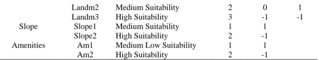
iii) Suitability indicator
Variable Code Description Level Effect coding River Riv1 Low Suitability 1 1 0
Riv2 Medium Suitability 2 0 1 Riv3 High Suitability 3 -1 -1 Land value Landv1 Low Suitability 1 1 0
Landm2 Medium Suitability 2 0 1 Landm3 High Suitability 3 -1 -1 Slope Slope1 Medium Suitability 1 1
Slope2 High Suitability 2 -1 Amenities Am1 Medium Low Suitability 1 1
Am2 High Suitability 2 -1
RESULTS
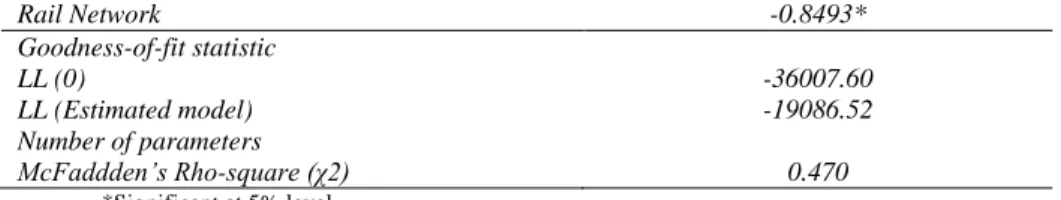
Maximum likelihood was used to estimate the model. The model was estimated using econometric software STATA version 10.0. The estimated parameters shown in Table 2. As one would expect, examining the result for firms located outside of CBD verify that firm types agriculture, mining, electricity, gas and water, and transport are mostly located outside of the CBD. One surprise result is that finance firms are also mostly located outside the CBD. This result is odd and seems at variance with CBDs around the world where finance firms are invariably located in the very heart of the CBD. Is it because such firms, e.g. banks, has many branches, outlets and ATMs located near other businesses outside the CBD for convenience of serving their customers, with perhaps only their HQ and a few branches located within the CBD.
Meanwhile, manufacturing, construction and wholesale firms’ type are located in the CBD area. This result also seems a little surprising. Manufacturing and construction firms often involve heavy bulk materials, and often require very large items for transport that are difficult to maneuver within the confines of generally narrower and more crowded road arterials in the CBD with far greater impedance factors (e.g. Not only traffic congestion and tight corners, but traffic lights and pedestrian crossings) than outside the CBD. However, in this case, this result might not surprising because the only office firm of these sectors was examined.
Table 2: Parameter estimates for firm location by type
Location Parameter Estimates
Agriculture 0.2152*
Mining 0.4033*
Manufacturing -0.2574*
Electric, Gas & Water 0.2361*
Construction -0.6089*
Wholesale -0.1126*
Transportation 0.1425*
Finance 0.2155*
Community Services (base type)
Amenities -1.2921*
Slope -0.0418
River1 -0.0263
River2 0.0496
Landvalue1 0.0198
Landvalue2 -0.0167
A Discrete Choice Model for Firm Location Decision
Rail Network -0.8493*
Goodness-of-fit statistic LL (0)
LL (Estimated model) Number of parameters
McFaddden’s Rho-square (χ2)
-36007.60 -19086.52
0.470 *Significant at 5% level
Analyzing the influence of the accessibility indicator, most of the firms in the CBD area hold the negative coefficient which show them co-located nearby. For the stability indicator, the details were analyzed by using interaction effects.
INTERACTION EFFECTS
In order to investigate more detail on a firm’slocation, a firm’s type and the suitability of its address inside or outside of the CBD, the interaction effect on the firm location model was performed. Interaction effects can be defined as an influence that one factor has on the other factor whereby it has a contribution of two or more variables that join together. In this interaction effect, the combination of the attributes will give an extra positive or negative effect to an alternative utility (Grigolon et.al, 2012).
In order to investigate the effects, a model containing interaction between a firm’s types and location's suitability was devised. First, a model containing three-level suitability (high, medium and low) was applied. However, since it was found after running the model that the three levels were not significant, the model was simplified by merging medium and low level into only two levels (high and medium/low). Table 3 shows the result of the interaction effects.
Table 3: Result of interaction effect on firm type and the suitability
Interaction effects Parameter Estimate
Interaction between predictor 1.Firm type: Agriculture
Agriculture and river1 -0.4184*
Agriculture and river2 0.7541*
Agriculture and rail1 0.2197*
Agriculture and rail2 0.0755*
Agriculture and node1 -0.2398*
Agriculture and node2 -0.0960*
Agriculture and land value1 -0.5997*
Agriculture and land value2 0.3518*
Agriculture and land mark1 0.0882*
Agriculture and land mark2 -0.5318*
Agriculture and slope -0.0550*
Agriculture and road -0.3016*
Agriculture and amenities 2.Firm type: Mining
Mining and river1 0.1433*
Mining and river2 -0.3153*
Mining and rail1 0.2382*
Mining and rail2 -0.0788*
Mining and node2 0.1972*
Mining and land value1 0.4770*
Mining and land value2 -0.1246*
Mining and land mark1 -0.0344
Mining and land mark2 0.4663*
Mining and slope
Mining and road -0.0836*
Mining and amenities 3.Firm type: Manufacturing
Manufacturing and river1 -0.0003
Manufacturing and river2 -0.0411
Manufacturing and rail1 -0.1127*
Manufacturing and rail2 0.0799*
Manufacturing and node1 0.0287
Manufacturing and node2 0.0391
Manufacturing and land value1 -0.0331
Manufacturing and land value2 0.0953*
Manufacturing and land mark1 -0.1087*
Manufacturing and land mark2 0.0759*
Manufacturing and slope 0.0045
Manufacturing and road -0.1570*
Manufacturing and amenities 0.3628*
4.Firm type: Electric, Gas & Water
Electric, Gas & Water and river1 -0.4659*
Electric, Gas & Water and river2 0.6729*
Electric, Gas & Water and rail1 0.1085*
Electric, Gas & Water and rail2 -0.8672*
Electric, Gas & Water and node1 0.4973*
Electric, Gas & Water and node2 -0.3403*
Electric, Gas & Water and land value1 0.0273
Electric, Gas & Water and land value2 -0.3197*
Electric, Gas & Water and land mark1 -0.0380
Electric, Gas & Water and land mark2 0.1587*
Electric, Gas & Water and slope 1.5167*
Electric, Gas & Water and road 0.4172
Electric, Gas & Water and amenities -2.0837*
5.Firm type: Construction
Construction and river1 0.4630*
Construction and river2 -0.4446*
Construction and rail1 -0.0729*
Construction and rail2 0.2369*
Construction and node1 -0.0581*
Construction and node2 0.0137
Construction and land value1 -0.0129
Construction and land value2 -0.0379
Construction and land mark1 -0.0403
Construction and land mark2 -0.1467*
A Discrete Choice Model for Firm Location Decision
Wholesale and river1 0.1517*
Wholesale and river2 -0.2534*
Wholesale and rail1 -0.1592*
Wholesale and rail2 0.1982*
Wholesale and node1 -0.0222
Wholesale and node2 -0.0030
Wholesale and land value1 -0.0447
Wholesale and land value2 0.0678*
Wholesale and land mark1 -0.0174
Wholesale and land mark2 0.0146
Wholesale and slope -0.2304*
Wholesale and road 0.0970*
Wholesale and amenities 0.5383*
7.Firm type: Transportation
Transportation and river1 -0.1253*
Transportation and river2 0.0373
Transportation and rail1 0.0697*
Transportation and rail2 -0.0118
Transportation and node1 -0.1926*
Transportation and node2 0.0867*
Transportation and land value1 0.0291
Transportation and land value2 0.0153
Transportation and land mark1 0.0836*
Transportation and land mark2 0.0329
Transportation and slope 0.0622*
Transportation and road 0.0843*
Transportation and amenities 8.Firm type: Finance
Finance and river1 0.0169
Finance and river2 -0.1409*
Finance and rail1 -0.1440*
Finance and rail2 0.2059*
Finance and node1 0.0283
Finance and node2 -0.0061
Finance and land value1 0.0243
Finance and land value2 0.0353
Finance and land mark1 0.0230
Finance and land mark2 -0.0416
Finance and slope -0.3507*
Finance and road 0.0148
Finance and amenities 0.6308*
*Significant at 5% level
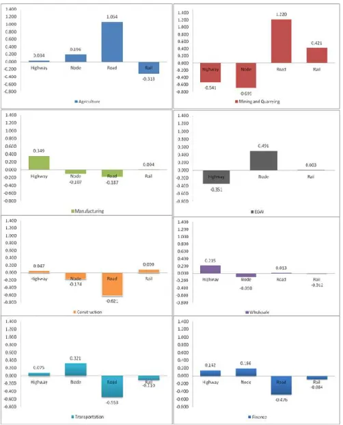
Interaction effect on firm’s type and accessibility measure
It is also interesting to examine and interpret the interaction effects on firms’ type and its accessibility measure. Figure 1 shows the results. The interaction for each type of firm, illustrated different influence to the accessibility location.
A Discrete Choice Model for Firm Location Decision
with the accessibility measure indicator - Mining and Quarrying, Transportation, and Finance.
CONCLUSION
The location of the firm is influenced by the accessibility and suitability indicators, especially in the CBD area. By using discrete choice modelling, the firm location in Kuala Lumpur by its sector can be identified. The results illustrated that some parameters were not significant and most probably due to the location choice of this research, limited only between areas inside and outside the CBD. Basically, the use of discrete choice models in the analysis of firm location decisions gives a foundation to facilitate town planners and decision makers to understand the firm location decisions in their region. It’s hoped that the model will contribute to better knowledge and practice and helps improving the decision-making process in the future.
REFERENCES
DiPasquale, D. & Wheaton, W.C. (1996). Urban Economics and Real Estate Markets,Prentice-Hall Incorporated: New Jersey.
Greene, W. (2008). Discrete Choice Modeling. New York, 2, 7–78.
Grigolon, A.B., Kemperman, A.D. a. M. & Timmermans, H.J.P., (2012). Student’s vacation travel: A reference dependent model of airline fares preferences. Journal of Air Transport Management, 18(1), pp.38-42.
Leitham, S., R. W. Mcquaid, and J. D. Nelson. (2000). The influence of transport on industrial location choice: A stated preference experiment. Transportation Research Part A: Policy and Practice, 34(7):515–535
Li, P. P. (2007). Towards an integrated theory of multinational evolution: the evidence of Chinese multinational enterprises as latecomers, Journal of International Management, vol. 13, pp. 296–318.
Parsons, G. (2004). Travel Cost Models. In P.Champ, K. Boyle, and T. Brown, eds. A Primer on Nonmarket Valuation. Boston: Kluwer Academic Publishers, pp. 269-330.