The Backpropagation Algorithm
7.1 Learning as gradient descent
We saw in the last chapter that multilayered networks are capable of com-puting a wider range of Boolean functions than networks with a single layer of computing units. However the computational effort needed for finding the correct combination of weights increases substantially when more parameters and more complicated topologies are considered. In this chapter we discuss a popular learning method capable of handling such large learning problems — the backpropagation algorithm. This numerical method was used by different research communities in different contexts, was discovered and rediscovered, until in 1985 it found its way into connectionist AI mainly through the work of the PDP group [382]. It has been one of the most studied and used algorithms for neural networks learning ever since.
In this chapter we present a proof of the backpropagation algorithm based on a graphical approach in which the algorithm reduces to a graph labeling problem. This method is not only more general than the usual analytical derivations, which handle only the case of special network topologies, but also much easier to follow. It also shows how the algorithm can be efficiently implemented in computing systems in which only local information can be transported through the network.
7.1.1 Differentiable activation functions
The backpropagation algorithm looks for the minimum of the error function in weight space using the method of gradient descent. The combination of weights which minimizes the error function is considered to be a solution of the learning problem. Since this method requires computation of the gradient of the error function at each iteration step, we must guarantee the conti-nuity and differentiability of the error function. Obviously we have to use a kind of activation function other than the step function used in perceptrons,
because the composite function produced by interconnected perceptrons is discontinuous, and therefore the error function too. One of the more popu-lar activation functions for backpropagation networks is the sigmoid, a real functionsc: IR→(0,1) defined by the expression
sc(x) = 1
1 + e−cx.
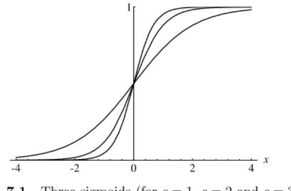
The constant c can be selected arbitrarily and its reciprocal 1/c is called the temperature parameter in stochastic neural networks. The shape of the sigmoid changes according to the value ofc, as can be seen in Figure 7.1. The graph shows the shape of the sigmoid for c = 1, c = 2 and c = 3. Higher values ofc bring the shape of the sigmoid closer to that of the step function and in the limitc→ ∞the sigmoid converges to a step function at the origin. In order to simplify all expressions derived in this chapter we set c= 1, but after going through this material the reader should be able to generalize all the expressions for a variablec. In the following we call the sigmoids1(x) just
s(x).
-4 -2 0 2 4 x
1
Fig. 7.1. Three sigmoids (forc= 1,c= 2 andc= 3)
The derivative of the sigmoid with respect to x, needed later on in this chapter, is
d dxs(x) =
e−x
(1 + e−x)2 =s(x)(1−s(x)).
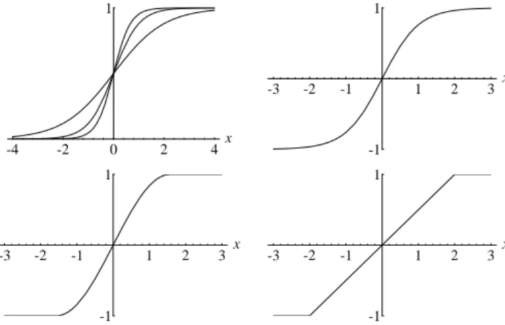
We have already shown that, in the case of perceptrons, a symmetrical activa-tion funcactiva-tion has some advantages for learning. An alternative to the sigmoid is the symmetrical sigmoidS(x) defined as
S(x) = 2s(x)−1 = 1−e
−x
1 + e−x.
This is nothing but the hyperbolic tangent for the argumentx/2 whose shape is shown in Figure 7.2 (upper right). The figure shows four types of continuous “squashing” functions. The ramp function (lower right) can also be used in
learning algorithms taking care to avoid the two points where the derivative is undefined.
-4 -2 0 2 4x
1
-3 -2 -1 1 2 3 x
-1 1
-3 -2 -1 1 2 3 x
-1 1
-3 -2 -1 1 2 3 x
-1 1
Fig. 7.2. Graphics of some “squashing” functions
Many other kinds of activation functions have been proposed and the back-propagation algorithm is applicable to all of them. A differentiable activation function makes the function computed by a neural network differentiable (as-suming that the integration function at each node is just the sum of the inputs), since the network itself computes only function compositions. The error function also becomes differentiable.
Figure 7.3 shows the smoothing produced by a sigmoid in a step of the error function. Since we want to follow the gradient direction to find the minimum of this function, it is important that no regions exist in which the error function is completely flat. As the sigmoid always has a positive derivative, the slope of the error function provides a greater or lesser descent direction which can be followed. We can think of our search algorithm as a physical process in which a small sphere is allowed to roll on the surface of the error function until it reaches the bottom.
7.1.2 Regions in input space
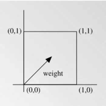
The sigmoid’s output range contains all numbers strictly between 0 and 1. Both extreme values can only be reached asymptotically. The computing units considered in this chapter evaluate the sigmoid using the net amount of exci-tation as its argument. Given weightsw1, . . . , wn and a bias−θ, a sigmoidal
unit computes for the inputx1, . . . , xn the output
1
1 + exp (Pni=1wixi−θ) .
Fig. 7.3. A step of the error function
A higher net amount of excitation brings the unit’s output nearer to 1. The continuum of output values can be compared to a division of the input space in a continuum of classes. A higher value of cmakes the separation in input space sharper.
(0,0) (0,1)
(1,0) (1,1)
weight
Fig. 7.4. Continuum of classes in input space
Note that the step of the sigmoid is normal to the vector (w1, . . . , wn,−θ)
so that the weight vector points in the direction in extended input space in which the output of the sigmoid changes faster.
7.1.3 Local minima of the error function
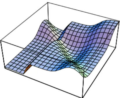
A price has to be paid for all the positive features of the sigmoid as activation function. The most important problem is that, under some circumstances, local minima appear in the error function which would not be there if the step function had been used. Figure 7.5 shows an example of a local minimum with a higher error level than in other regions. The function was computed for a single unit with two weights, constant threshold, and four input-output patterns in the training set. There is a valley in the error function and if
gradient descent is started there the algorithm will not converge to the global minimum.
Fig. 7.5. A local minimum of the error function
In many cases local minima appear because the targets for the outputs of the computing units are values other than 0 or 1. If a network for the computation of XOR is trained to produce 0.9 at the inputs (0,1) and (1,0) then the surface of the error function develops some protuberances, where local minima can arise. In the case of binary target values some local minima are also present, as shown by Lisboa and Perantonis who analytically found all local minima of the XOR function [277].
7.2 General feed-forward networks
In this section we show that backpropagation can easily be derived by linking the calculation of the gradient to a graph labeling problem. This approach is not only elegant, but also more general than the traditional derivations found in most textbooks. General network topologies are handled right from the beginning, so that the proof of the algorithm is not reduced to the multilayered case. Thus one can have it both ways, more general yet simpler [375]. 7.2.1 The learning problem
Recall that in our general definition a feed-forward neural network is a com-putational graph whose nodes are computing units and whose directed edges transmit numerical information from node to node. Each computing unit is ca-pable of evaluating a single primitive function of its input. In fact the network represents a chain of function compositions which transform an input to an output vector (called a pattern). The network is a particular implementation of a composite function from input to output space, which we call thenetwork function. The learning problem consists of finding the optimal combination
of weights so that the network function ϕapproximates a given function f as closely as possible. However, we are not given the functionf explicitlybut only implicitly through some examples.
Consider a feed-forward network withninput andmoutput units. It can consist of any number of hidden units and can exhibit any desired feed-forward connection pattern. We are also given a training set {(x1,t1), . . . ,(xp,tp)}
consisting ofpordered pairs ofn- andm-dimensional vectors, which are called the input and output patterns. Let the primitive functions at each node of the network be continuous and differentiable. The weights of the edges are real numbers selected at random. When the input patternxifrom the training set
is presented to this network, it produces an outputoidifferent in general from
the target ti. What we want is to make oi and ti identical for i = 1, . . . , p,
by using a learning algorithm. More precisely, we want to minimize the error function of the network, defined as
E=1 2
p X i=1
koi−tik2.
After minimizing this function for the training set, new unknown input pat-terns are presented to the network and we expect it tointerpolate. The network must recognize whether a new input vector is similar to learned patterns and produce a similar output.
The backpropagation algorithm is used to find a local minimum of the error function. The network is initialized with randomly chosen weights. The gradient of the error function is computed and used to correct the initial weights. Our task is to compute this gradient recursively.
network +
network
+
. . .
xi1
xi2
xin
Ei
1
2(oi1−ti1)2
1
2(oi2−ti2)2
1
2(oim−tim) 2
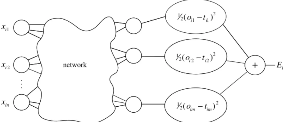
Fig. 7.6.Extended network for the computation of the error function
The first step of the minimization process consists of extending the net-work, so that it computes the error function automatically. Figure 7.6 shows
how this is done. Every one of thej output units of the network is connected to a node which evaluates the function 12(oij−tij)2, whereoij andtij denote
thej-th component of the output vectoroi and of the targetti. The outputs
of the additionalm nodes are collected at a node which adds them up and gives the sumEias its output. The same network extension has to be built for
each pattern ti. A computing unit collects all quadratic errors and outputs
their sum E1+· · ·+Ep. The output of this extended network is the error
functionE.
We now have a network capable of calculating the total error for a given training set. The weights in the network are the only parameters that can be modified to make the quadratic error E as low as possible. Because E is calculated by the extended network exclusively through composition of the node functions, it is a continuous and differentiable function of the`weights w1, w2, . . . , w` in the network. We can thus minimize E by using an iterative
process of gradient descent, for which we need to calculate the gradient ∇E= (∂E
∂w1,
∂E ∂w2, . . . ,
∂E ∂w`).
Each weight is updated using the increment ∆wi=−γ∂E
∂wi
fori= 1, . . . , `,
whereγrepresents a learning constant, i.e., a proportionality parameter which defines the step length of each iteration in the negative gradient direction.
With this extension of the original network the whole learning problem now reduces to the question of calculating the gradient of a network function with respect to its weights. Once we have a method to compute this gradient, we can adjust the network weights iteratively. In this way we expect to find a minimum of the error function, where∇E= 0.
7.2.2 Derivatives of network functions
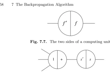
Now forget everything about training sets and learning. Our objective is to find a method for efficiently calculating the gradient of a one-dimensional network function according to the weights of the network. Because the network is equivalent to a complex chain of function compositions, we expect the chain rule of differential calculus to play a major role in finding the gradient of the function. We take account of this fact by giving the nodes of the network a composite structure. Each node now consists of a left and a right side, as shown in Figure 7.7. We call this kind of representation a B-diagram (for backpropagation diagram).
The right side computes the primitive function associated with the node, whereas the left side computes the derivative of this primitive function for the same input.
f
′
f
Fig. 7.7. The two sides of a computing unit
s
′
s +
1
Fig. 7.8. Separation of integration and activation function
Note that the integration function can be separated from the activation function by splitting each node into two parts, as shown in Figure 7.8. The first node computes the sum of the incoming inputs, the second one the activation functions. The derivative ofsiss0 and the partial derivative of the sum ofn arguments with respect to any one of them is just 1. This separation simplifies our discussion, as we only have to think of a single function which is being computed at each node and not of two.
The network is evaluated in two stages: in the first one, the feed-forward step, information comes from the left and each unit evaluates its primitive function f in its right side as well as the derivative f0 in its left side. Both
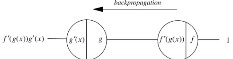
results are stored in the unit, but only the result from the right side is transmit-ted to the units connectransmit-ted to the right. The second step, the backpropagation step, consists in running the whole network backwards, whereby the stored results are now used. There are three main cases which we have to consider. First case: function composition
The B-diagram of Figure 7.9 contains only two nodes. In the feed-forward step, incoming information into a unit is used as the argument for the evaluation of the node’s primitive function and its derivative. In this step the network computes the composition of the functions f and g. Figure 7.10 shows the state of the network after the feed-forward step. The correct result of the function composition has been produced at the output unit and each unit has stored some information on its left side.
In the backpropagation step the input from the right of the network is the constant 1. Incoming information to a node is multiplied by the value stored in its left side. The result of the multiplication is transmitted to the next unit to the left. We call the result at each node the traversing value at this node. Figure 7.11 shows the final result of the backpropagation step, which isf0(g(x))g0(x), i.e., the derivative of the function compositionf(g(x))
x g ′ g f ′ f
Fig. 7.9. Network for the composition of two functions
x
function composition
f(g(x)) g
′
g (x) f ′ (g(x)) f
Fig. 7.10. Result of the feed-forward step
implemented by this network. The backpropagation step provides an imple-mentation of the chain rule. Any sequence of function compositions can be evaluated in this way and its derivative can be obtained in the backpropa-gation step. We can think of the network as being used backwards with the input 1, whereby at each node the product with the value stored in the left side is computed.
g
′
g (x) f ′ (g(x)) f 1 backpropagation
′
f (g(x))g ′ (x)
Fig. 7.11. Result of the backpropagation step
+ 1 1 x
function composition
f1
f2
f1(x)+f2(x) ′
f 1(x)
′
f 2(x)
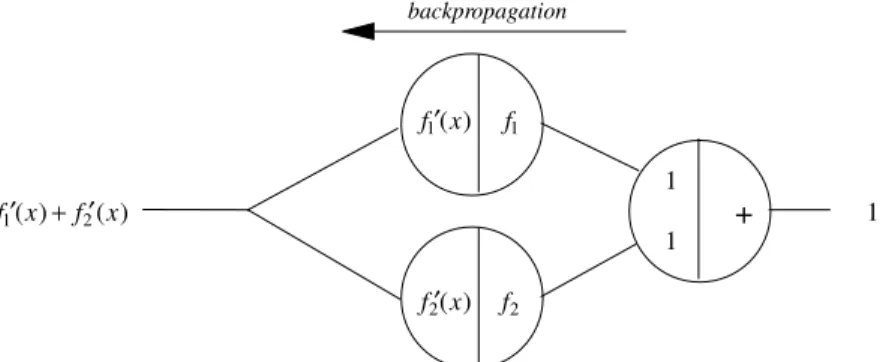
Second case: function addition
The next case to consider is the addition of two primitive functions. Fig-ure 7.12 shows a network for the computation of the addition of the functions f1and f2 . The additional node has been included to handle the addition of
the two functions. The partial derivative of the addition function with respect to any one of the two inputs is 1. In the feed-forward step the network com-putes the resultf1(x) +f2(x). In the backpropagation step the constant 1 is
fed from the left side into the network. All incoming edges to a unit fan out the traversing value at this node and distribute it to the connected units to the left. Where two right-to-left paths meet, the computed traversing values are added. Figure 7.13 shows the resultf0
1(x) +f20(x) of the backpropagation
step, which is the derivative of the function additionf1+f2 evaluated atx.
A simple proof by induction shows that the derivative of the addition of any number of functions can be handled in the same way.
+ 1 1 backpropagation
f1
f2 ′
f 1(x)
′
f 2(x)
1
′
f 1(x)+ ′ f 2(x)
Fig. 7.13. Result of the backpropagation step
w
x wx
backpropagation w
1 feed-forward
w
Third case: weighted edges
Weighted edges could be handled in the same manner as function composi-tions, but there is an easier way to deal with them. In the feed-forward step the incoming informationxis multiplied by the edge’s weight w. The result is wx. In the backpropagation step the traversing value 1 is multiplied by the weight of the edge. The result is w, which is the derivative of wx with respect to x. From this we conclude that weighted edges are used in exactly the same way in both steps: they modulate the information transmitted in each direction by multiplying it by the edges’ weight.
7.2.3 Steps of the backpropagation algorithm
We can now formulate the complete backpropagation algorithm and prove by induction that it works in arbitrary feed-forward networks with differentiable activation functions at the nodes. We assume that we are dealing with a network with a single input and a single output unit.
Algorithm 7.2.1 Backpropagation algorithm.
Consider a network with a single real input xand network function F. The derivativeF0(x) is computed in two phases:
Feed-forward: the input x is fed into the network. The primitive func-tions at the nodes and their derivatives are evaluated at each node. The derivatives are stored.
Backpropagation: the constant 1 is fed into the output unit and the network is run backwards. Incoming information to a node is added and the result is multiplied by the value stored in the left part of the unit. The result is transmitted to the left of the unit. The result collected at the input unit is the derivative of the network function with respect tox.
The following proposition shows that the algorithm is correct.
Proposition 11.Algorithm 7.2.1 computes the derivative of the network function F with respect to the inputxcorrectly.
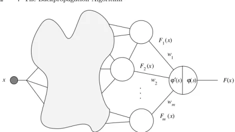
Proof. We have already shown that the algorithm works for units in series, units in parallel and also for weighted edges. Let us make the induction as-sumption that the algorithm works for any feed-forward network with n or fewer nodes. Consider now the B-diagram of Figure 7.15, which containsn+ 1 nodes. The feed-forward step is executed first and the result of the single output unit is the network functionF evaluated atx. Assume thatm units, whose respective outputs are F1(x), . . . , Fm(x) are connected to the output
F(x)
F1(x)
F
2(x)
Fm(x)
w
1
w
2
wm
x ϕ ′ (s) ϕ(s)
. . .
Fig. 7.15. Backpropagation at the last node
F(x) =ϕ(w1F1(x) +w2F2(x) +· · ·+wmFm(x)).
The derivative ofF atxis thus F0(x) =ϕ0(s)(w
1F10(x) +w2F20(x) +· · ·+wmFm0 (x)),
where s = ϕ(w1F1(x) +w2F2(x) +· · ·+wmFm(x)). The subgraph of the
main graph which includes all possible paths from the input unit to the unit whose output is F1(x) defines a subnetwork whose network function is F1
and which consists of nor fewer units. By the induction assumption we can calculate the derivative of F1 at x, by introducing a 1 into the unit and
running the subnetwork backwards. The same can be done with the units whose outputs areF2(x), . . . , Fm(x). If instead of 1 we introduce the constant ϕ0(s) and multiply it by w
1 we get w1F10(x)ϕ0(s) at the input unit in the
backpropagation step. Similarly we getw2F20(x)ϕ0(s), . . . , wmFm0 (x)ϕ0(s) for
the rest of the units. In the backpropagation step with the whole network we add thesem results and we finally get
ϕ0(s)(w1F10(x) +w2F20(x) +· · ·+wmFm0 (x))
which is the derivative of F evaluated at x. Note that introducing the con-stantsw1ϕ0(s), . . . , wmϕ0(s) into themunits connected to the output unit can
be done by introducing a 1 into the output unit, multiplying by the stored valueϕ0(s) and distributing the result to themunits through the edges with
weightsw1, w2, . . . , wm. We are in fact running the network backwards as the
backpropagation algorithm demands. This means that the algorithm works with networks ofn+ 1 nodes and this concludes the proof. 2
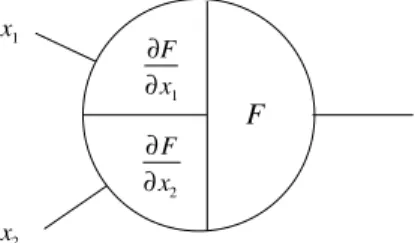
Implicit in the above analysis is that all inputs to a node are added be-fore the one-dimensional activation function is computed. We can consider
also activation functions f of several variables, but in this case the left side of the unit stores all partial derivatives of f with respect to each variable. Figure 7.16 shows an example for a functionf of two variablesx1andx2,
de-livered through two different edges. In the backpropagation step each stored partial derivative is multiplied by the traversing value at the node and trans-mitted to the leftthrough its own edge. It is easy to see that backpropagation still works in this more general case.
∂F
∂x1
∂F
∂x2 F
x2 x1
Fig. 7.16. Stored partial derivatives at a node
The backpropagation algorithm also works correctly for networks with more than one input unit in which several independent variables are involved. In a network with two inputs for example, where the independent variablesx1
and x2 are fed into the network, the network result can be calledF(x1, x2).
The network function now has two arguments and we can compute the par-tial derivative of F with respect to x1 orx2. The feed-forward step remains
unchanged and all left side slots of the units are filled as usual. However, in the backpropagation step we can identify two subnetworks: one consists of all paths connecting the first input unit to the output unit and another of all paths from the second input unit to the output unit. By applying the back-propagation step in the first subnetwork we get the partial derivative of F with respect to x1 at the first input unit. The backpropagation step on the
second subnetwork yields the partial derivative ofF with respect tox2 at the
second input unit. Note that we can overlap both computations and perform a single backpropagation step over the whole network. We still get the same results.
7.2.4 Learning with backpropagation
We consider again the learning problem for neural networks. Since we want to minimize the error functionE, which depends on the network weights, we have to deal with all weights in the network one at a time. The feed-forward step is computed in the usual way, but now we also store the output of each unit in its right side. We perform the backpropagation step in the extended network that computes the error function and we then fix our attention on one of the weights, saywij whose associated edge points from thei-th to the
j-th node in the network. This weight can be treated as an input channel into the subnetwork made of all paths starting at wij and ending in the single
output unit of the network. The information fed into the subnetwork in the feed-forward step was oiwij, where oi is the stored output of unit i. The
backpropagation step computes the gradient ofE with respect to this input, i.e.,∂E/∂oiwij. Since in the backpropagation stepoi is treated as a constant,
we finally have
∂E ∂wij
=oi ∂E ∂oiwij
.
Summarizing, the backpropagation step is performed in the usual way. All subnetworks defined by each weight of the network can be handled simulta-neously, but we now store additionally at each nodei:
• The outputoi of the node in the feed-forward step.
• The cumulative result of the backward computation in the backpropaga-tion step up to this node. We call this quantity thebackpropagated error. If we denote the backpropagated error at thej-th node byδj, we can then
express the partial derivative ofE with respect towij as: ∂E
∂wij =oiδj.
Once all partial derivatives have been computed, we can perform gradient descent by adding to each weightwij the increment
∆wij =−γoiδj.
This correction step is needed to transform the backpropagation algorithm into a learning method for neural networks.
This graphical proof of the backpropagation algorithm applies to arbitrary feed-forward topologies. The graphical approach also immediately suggests hardware implementation techniques for backpropagation.
7.3 The case of layered networks
An important special case of feed-forward networks is that of layered networks with one or more hidden layers. In this section we give explicit formulas for the weight updates and show how they can be calculated using linear algebraic operations. We also show how to label each node with the backpropagated error in order to avoid redundant computations.
7.3.1 Extended network
We will consider a network withninput sites,khidden, andmoutput units. The weight between input site i and hidden unitj will be called w(1)ij . The weight between hidden unitiand output unitj will be calledw(2)ij . The bias
−θ of each unit is implemented as the weight of an additional edge. Input vectors are thus extended with a 1 component, and the same is done with the output vector from the hidden layer. Figure 7.17 shows how this is done. The weight between the constant 1 and the hidden unitj is calledw(1)n+1,j and the
weight between the constant 1 and the output unitj is denoted byw(2)k+1,j.
n input sites
m output units
1
1 hidden units
connection matrix
W1
connection matrix W2 wn+1,
(1)
wk+1,
site n+1
k
k m
(2)
.
.
.
.
.
.
.
.
.
Fig. 7.17. Notation for the three-layered network
There are (n+ 1)×k weights between input sites and hidden units and (k+ 1)×mbetween hidden and output units. LetW1denote the (n+ 1)×k
matrix with componentw(1)ij at thei-th row and thej-th column. Similarly
let W2 denote the (k+ 1)×m matrix with components w(2)ij . We use an
overlined notation to emphasize that the last row of both matrices corresponds to the biases of the computing units. The matrix of weights without this last row will be needed in the backpropagation step. The n-dimensional input vectoro= (o1, . . . , on) is extended, transforming it to ˆo= (o1, . . . , on,1). The
excitationnetj of thej-th hidden unit is given by netj=
n+1
X i=1
wij(1)oˆi.
o(1)j =s n+1
X i=1
w(1)ij oˆi !
.
The excitation of all units in the hidden layer can be computed with the vector-matrix multiplication ˆoW1. The vectoro(1) whose components are the
outputs of the hidden units is given by o(1) =s(ˆoW
1),
using the convention of applying the sigmoid to each component of the ar-gument vector. The excitation of the units in the output layer is computed using the extended vector ˆo(1)= (o(1)
1 , . . . , o (1)
k ,1). The output of the network
is them-dimensional vectoro(2), where
o(2)=s(ˆo(1)W2).
These formulas can be generalized for any number of layers and allow direct computation of the flow of information in the network with simple matrix operations.
7.3.2 Steps of the algorithm
Figure 7.18 shows the extended network for computation of the error function. In order to simplify the discussion we deal with a single input-output pair (o,t) and generalize later toptraining examples. The network has been extended with an additional layer of units. The right sides compute the quadratic de-viation 12(o(2)i −ti) for the i-th component of the output vector and the left
sides store (o(2)i −ti). Each output unit i in the original network computes
the sigmoid sand produces the output o(2)i . Addition of the quadratic devi-ations gives the errorE. The error function for pinput-output examples can be computed by creatingpnetworks like the one shown, one for each training pair, and adding the outputs of all of them to produce the total error of the training set.
After choosing the weights of the network randomly, the backpropagation algorithm is used to compute the necessary corrections. The algorithm can be decomposed in the following four steps:
i) Feed-forward computation
ii) Backpropagation to the output layer iii) Backpropagation to the hidden layer iv) Weight updates
The algorithm is stopped when the value of the error function has become sufficiently small.
E
′
s s
′
s s
′
s s
output units
i-th hidden unit
+
oi( 1)o1( 2)
o2( 2)
1 2(o1
( 2)−
t1)2 (o1(2)−t1)
1 2(o2
( 2)
−t2)2 (o2(2)−t2)
1
2(om( 2)−tm)2
(om(2)−tm)2
.
.
.
.
.
.
om( 2) wim( 2)
Fig. 7.18. Extended multilayer network for the computation ofE
First step: feed-forward computation
The vectorois presented to the network. The vectorso(1) ando(2) are
com-puted and stored. The evaluated derivatives of the activation functions are also stored at each unit.
Second step: backpropagation to the output layer
We are looking for the first set of partial derivatives ∂E/∂wij(2). The
back-propagation path from the output of the network up to the output unit j is shown in the B-diagram of Figure 7.19.
+
1 1
j-th output unit
i-th hidden unit quadratic error of the
j-th component backpropagated error up to unit j
backpropagation
oi( 1)
wij( 2)
o( 2)j (1−o( 2)j ) o( 2)j (1−o( 2)j )(oj(2)−tj)
o( 2)j −tj
( ) 1
2 oj
( 2)
−tj
( )2
o( 2)j
From this path we can collect by simple inspection all the multiplicative terms which define the backpropagated errorδ(2)j . Therefore
δ(2)j =o(2)j (1−o(2)j )(o(2)j −tj),
and the partial derivative we are looking for is ∂E
∂wij(2)
= [o(2)j (1−o
(2)
j )(o
(2)
j −tj)]o(1)i =δ
(2)
j o
(1)
i .
Remember that for this last step we consider the weightw(2)ij to be a variable
and its inputoi(1) a constant.
oi(1) δj(2)
wij( 2)
Fig. 7.20. Input and backpropagated error at an edge
Figure 7.20 shows the general situation we find during the backpropagation algorithm. At the input side of the edge with weightwij we haveo(1)i and at
the output side the backpropagated errorδ(2)j .
Third step: backpropagation to the hidden layer
Now we want to compute the partial derivatives ∂E/∂wij(1). Each unitj in
the hidden layer is connected to each unitqin the output layer with an edge of weight wjq(2), for q = 1, . . . , m. The backpropagated error up to unit j in
the hidden layer must be computed taking into account all possible backward paths, as shown in Figure 7.21. The backpropagated error is then
δ(1)j =o
(1)
j (1−o
(1)
j ) m X q=1
wjq(2)δ(2)q .
Therefore the partial derivative we are looking for is ∂E
∂w(1)ij =δ
(1)
j oi.
The backpropagated error can be computed in the same way for any number of hidden layers and the expression for the partial derivatives ofE keeps the same analytic form.
Σ
hidden unit j
backpropagated error to the j-th hidden unit
backpropagation
input site i
backpropagated error
o( 1)j wij(1)
oi
wj( 2)1 wj( 2)2
wjm( 2)
δ1 (2)
δ2 (2)
δm
(2)
o( 1)j (1−oj(1)) wjq( 2)δq(2) q=1
m
o( 1)j (1−oj(1))
.
.
.
.
.
.
Fig. 7.21. All paths up to input sitei
Fourth step: weight updates
After computing all partial derivatives the network weights are updated in the negative gradient direction. A learning constantγ defines the step length of the correction. The corrections for the weights are given by
∆wij(2)=−γo(1)i δj(2), fori= 1, . . . , k+ 1;j = 1, . . . , m, and
∆w(1)ij =−γoiδj(1), fori= 1, . . . , n+ 1;j= 1, . . . , k,
where we use the convention that on+1 = o(1)k+1 = 1. It is very important
to make the corrections to the weights only after the backpropagated error has been computed for all units in the network. Otherwise the corrections become intertwined with the backpropagation of the error and the computed corrections do not correspond any more to the negative gradient direction. Some authors fall in this trap [16]. Note also that some books define the backpropagated error as thenegativetraversing value in the network. In that case the update equations for the network weights do not have a negative sign (which is absorbed by the deltas), but this is a matter of pure convention. More than one training pattern
In the case of p >1 input-output patterns, an extended network is used to compute the error function for each of them separately. The weight corrections
are computed for each pattern and so we get, for example, for weightw(1)ij the corrections
∆1w(1)ij , ∆2wij(1), . . . , ∆pwij(1).
The necessary update in the gradient direction is then ∆w(1)ij =∆1w(1)ij +∆2w(1)ij +· · ·+∆pw(1)ij .
We speak ofbatch or off-lineupdates when the weight corrections are made in this way. Often, however, the weight updates are made sequentially after each pattern presentation (this is called on-line training). In this case the corrections do not exactly follow the negative gradient direction, but if the training patterns are selected randomly the search direction oscillates around the exact gradient direction and, on average, the algorithm implements a form of descent in the error function. The rationale for using on-line training is that adding some noise to the gradient direction can help to avoid falling into shallow local minima of the error function. Also, when the training set consists of thousands of training patterns, it is very expensive to compute the exact gradient direction since each epoch (one round of presentation of all patterns to the network) consists of many feed-forward passes and on-line training becomes more efficient [391].
7.3.3 Backpropagation in matrix form
We have seen that the graph labeling approach for the proof of the backpropa-gation algorithm is completely general and is not limited to the case of regular layered architectures. However this special case can be put into a form suitable for vector processors or special machines for linear algebraic operations.
We have already shown that in a network with a hidden and an output layer (n,k and m units) the inputoproduces the output o(2) =s(ˆo(1)W
2)
where o(1) =s(ˆoW
1). In the backpropagation step we only need the firstn
rows of matrixW1. We call thisn×kmatrixW1. Similarly, thek×mmatrix
W2is composed of the firstkrows of the matrixW2. We make this reduction
because we do not need to backpropagate any values to the constant inputs corresponding to each bias.
The derivatives stored in the feed-forward step at thek hidden units and themoutput units can be written as the two diagonal matrices
D2=
o(2)1 (1−o (2)
1 ) 0 · · · 0
0 o(2)2 (1−o (2)
2 )· · · 0
..
. ... . .. ...
0 0 · · ·o(2)m(1−o(2)m) ,
D1=
o(1)1 (1−o(1)1 ) 0 · · · 0 0 o(1)2 (1−o(1)2 )· · · 0 ..
. ... . .. ...
0 0 · · ·o(1)k (1−o(1)k ) .
Define the vectoreof the stored derivatives of the quadratic deviations as
e=
(o(2)1 −t1)
(o(2)2 −t2)
.. . (o(2)m −tm)
Them-dimensional vectorδ(2) of the backpropagated error up to the output
units is given by the expression
δ(2)=D2e.
Thek-dimensional vector of the backpropagated error up to the hidden layer is
δ(1)=D1W2δ(2).
The corrections for the matricesW1 andW2 are then given by
∆WT2 =−γδ(2)ˆo1 (7.1)
and
∆WT1 =−γδ(1)oˆ. (7.2)
The only necessary operations are matrix, matrix-vector, and vector-vector multiplications. In Chap. 16 we describe computer architectures op-timized for this kind of operation. It is easy to generalize these equations for` layers of computing units. Assume that the connection matrix between layeriandi+ 1 is denoted by Wi+1 (layer 0 is the layer of input sites). The
backpropagated error to the output layer is then
δ(`)=D`e.
The backpropagated error to the i-th computing layer is defined recursively by
δ(i)=DiWi+1δ(i+1), fori= 1, . . . , `−1.
or alternatively
δ(i)=DiWi+1· · ·W`−1D`−1W`D`e.
The corrections to the weight matrices are computed in the same way as for two layers of computing units.
7.3.4 The locality of backpropagation
We can now prove using a B-diagram that addition is the only integration function which preserves the locality of learning when backpropagation is used.
f ′ f
*
a
b a b f′(a b)b
backpropagation
f′(a b)a
Fig. 7.22. Multiplication as integration function
In the networks we have seen so far the backpropagation algorithm ex-ploits only local information. This means that only information which arrives from an input line in the feed-forward step is stored at the unit and sent back through the same line in the backpropagation step. An example can make this point clear. Assume that the integration function of a unit is multiplication and its activation function isf. Figure 7.22 shows a split view of the compu-tation: two inputsaandbcome from two input lines, the integration function responds with the productaband this result is passed as argument tof. With backpropagation we can compute the partial derivative off(ab) with respect to aand with respect tob. But in this case the valueb must be transported back through the upper edge and the value a through the lower one. Since b arrived through the other edge, the locality of the learning algorithm has been lost. The question is which kinds of integration functions preserve the locality of learning. The answer is given by the following proposition. Proposition 12.In a unit withninputsx1, . . . , xnonly integration functions
of the form
I(x1, . . . , xn) =F1(x1) +F2(x2) +· · ·+Fn(xn) +C,
whereCis a constant, guarantee the locality of the backpropagation algorithm in the sense that at an edge i6=j no information aboutxj has to be explicitly
stored.
Proof. Let the integration function of the unit be the function I of n argu-ments. If, in the backpropagation step, only a function fi of the variablexi
can be stored at the computing unit in order to be transmitted through the i-th input line in the backpropagation step, then we know that
∂I ∂xi
Therefore by integrating these equations we obtain:
I(x1, x2, . . . , xn) =F1(x1) +G1(x2, . . . , xn), I(x1, x2, . . . , xn) =F2(x2) +G2(x2, . . . , xn),
.. .
I(x1, x2, . . . , xn) =Fn(xn) +Gn(x2, . . . , xn),
whereFidenotes the integral offiandG1, . . . , Gnare real functions ofn−1
arguments. Since the functionI has a unique form, the only possibility is I(x1, x2, . . . , xn) =F1(x1) +F2(x2) +· · ·+Fn(xn) +C
where C is a constant. This means that information arriving from each line can be preprocessed by theFifunctions and then has to be added. Therefore
only integration functions with this form preserve locality. 2 7.3.5 Error during training
We discussed the form of the error function for the XOR problem in the last chapter. It is interesting to see how backpropagation performs when con-fronted with this problem. Figure 7.23 shows the evolution of the total error during training of a network of three computing units. After 600 iterations the algorithm found a solution to the learning problem. In the figure the error falls fast at the beginning and end of training. Between these two zones lies a region in which the error function seems to be almost flat and where progress is slow. This corresponds to a region which would be totally flat if step func-tions were used as activation funcfunc-tions of the units. Now, using the sigmoid, this region presents a small slope in the direction of the global minimum.
In the next chapter we discuss how to make backpropagation converge faster, taking into account the behavior of the algorithm at the flat spots of the error function.
7.4 Recurrent networks
The backpropagation algorithm can also be extended to the case of recurrent networks. To deal with this kind of systems we introduce a discrete time variablet. At timetall units in the network recompute their outputs, which are then transmitted at timet+ 1. Continuing in this step-by-step fashion, the system produces a sequence of output values when a constant or time varying input is fed into the network. As we already saw in Chap. 2, a recurrent network behaves like a finite automaton. The question now is how to train such an automaton to produce a desired sequence of output values.
0 0,1 0,2 0,3 0,4 0,5 0,6 0,7
XOR experiment
iterations error
600
0 300
Fig. 7.23. Error function for 600 iterations of backpropagation
7.4.1 Backpropagation through time
The simplest way to deal with a recurrent network is to consider a finite num-ber of iterations only. Assume for generality that a network of ncomputing units is fully connected and thatwij is the weight associated with the edge
from nodeito nodej. By unfolding the network at the time steps 1,2, . . . , T, we can think of this recurrent network as a feed-forward network withTstages of computation. At each time steptan external inputx(t) is fed into the net-work and the outputs (o(1t), . . . , o
(t)
n ) of all computing units are recorded. We
call then-dimensional vector of the units’ outputs at timetthe network state o(t). We assume that the initial values of all unit’s outputs are zero att= 0,
but the external input x(0) can be different from zero. Figure 7.24 shows a diagram of the unfolded network. This unfolding strategy which converts a recurrent network into a feed-forward network in order to apply the back-propagation algorithm is called backpropagation through time or just BPTT [383].
LetW stand for then×nmatrix of network weightswij. LetW0 stand
for them×nmatrix of interconnections betweenm input sites andn units. The feed-forward step is computed in the usual manner, starting with an initial m-dimensional external input x(0). At each time step t the network
stateo(t) (ann-dimensional row vector) and the vector of derivatives of the
activation function at each nodeo0(t)are stored. The error of the network can
be measured after each time step if a sequence of values is to be produced, or just after the final step T if only the final output is of importance. We will handle the first, more general case. Denote the difference between the n-dimensional targety(t) at timet and the output of the network bye(t) =
o(t)−y(t)T. This is ann-dimensional column vector, but in most cases we
unit 2
unit n
t = 1 t = 2 t = T
t = 0
(0) (1) (2) (T)
x x x x
(0) (1) (T)
o o o
unit 1
Fig. 7.24. Backpropagation through time
defineei(t) = 0 for each uniti, whose precise state is unimportant and which
can remain hidden from view.
w1≡w
w2≡w
Fig. 7.25. A duplicated weight in a network
Things become complicated when we consider that each weight in the network is present at each stage of the unfolded network. Until now we had only handled the case of unique weights. However, any network with repeated weights can easily be transformed into a network with unique weights. Assume that after the feed-forward step the state of the network is the one shown in Figure 7.25. Weight w is duplicated, but received different inputso1 and
o2 in the feed-forward step at the two different locations in the network.
The transformed network in Figure 7.26 is indistinguishable from the original network from the viewpoint of the results it produces. Note that the two edges associated with weightwnow have weight 1 and a multiplication is performed by the two additional units in the middle of the edges. In this transformed networkw appears only once and we can perform backpropagation as usual. There are two groups of paths, the ones coming from the first multiplier tow
w
*
*
Fig. 7.26. Transformed network
and the ones coming from the second. This means that we can just perform backpropagation as usual in the original network. At the first edge we obtain ∂E/∂w1, at the second∂E/∂w2, and sincew1 is the same variable asw2, the
desired partial derivative is ∂E
∂w =
∂E ∂w1
+ ∂E ∂w2
.
We can thus conclude in general that in the case of the same weight being associated with several edges, backpropagation is performed as usual for each of those edges and the results are simply added.
The backpropagation phase of BPTT starts from the right. The backprop-agated error at timeT is given by
δ(T)=D(T)e(T),
whereD(T)is then×ndiagonal matrix whose component at thei-th diagonal
element iso0 i
(T)
, i.e., the stored derivative of the i-th unit output at timeT. The backpropagated error at timeT−1 is given by
δ(T−1)=D(T−1)e(T−1)+D(T−1)WD(T)e(T),
where we have considered all paths from the computed errors at timeT and T −1 to each weight. In general, the backpropagated error at stage i, for i= 0, . . . , T−1 is
δ(i)=D(i)(e(i)+Wδ(i+1)).
The analytic expression for the final weight corrections are
∆WT =−γδ(1)ˆo(0)+· · ·+δ(T)oˆ(T−1) (7.3)
∆WT0 =−γ
where ˆo(1), . . . ,ˆo(T)denote the extended output vectors at steps 1, . . . , T and
WandW0 the extended matricesWandW0.
Backpropagation through time can be extended to the case of infinite time T. In this case we are interested in the limit value of the network’s state, on the assumption that the network’s state stabilizes to a fixpoint ˜o. Under some conditions over the activation functions and network topology such a fixpoint exists and its derivative can be calculated by backpropagation. The feed-forward step is repeated a certain number of times, until the network relaxes to a numerically stable state (with certain precision). The stored node’s outputs and derivatives are the ones computed in the last iteration. The network is then run backwards in backpropagation manner until it reaches a numerically stable state. The gradient of the network function with respect to each weight can then be calculated in the usual manner. Note that in this case, we do not need to store all intermediate values of outputs and derivatives at the units, only the final ones. This algorithm, called recurrent backpropagation, was proposed independently by Pineda [342] and Almeida [20].
7.4.2 Hidden Markov Models
Hidden Markov Models (HMM) form an important special type of recurrent network. A first-order Markov model is any system capable of assuming one of ndifferent states at timet. The system does not change its state at each time step deterministically but according to a stochastic dynamics. The probability of transition from thei-th to thej-th state at each step is given by 0≤aij ≤1
and does not depend on the previous history of transitions. These probabilities can be arranged in an n×n matrix A. We also assume that at each step the model emits one of m possible output values. We call the probability of emitting the k-th output value while in the i-th state bik. Starting from a
definite state at timet= 0, the system is allowed to run forT time units and the generated outputs are recorded. Each new run of the system generally produces a different sequence of output values. The system is called a HMM because only the emitted values, not the state transitions, can be observed.
An example may make this point clear. In speech recognition researchers postulate that the vocal tract shapes can be quantized in a discrete set of states roughly associated with the phonemes which compose speech. When speech is recorded the exact transitions in the vocal tract cannot be observed and only the produced sound can be measured at some predefined time intervals. These are the emissions, and the states of the system are the quantized configurations of the vocal tract. From the measurements we want to infer the sequence of states of the vocal tract, i.e., the sequence of utterances which gave rise to the recorded sounds. In order to make this problem manageable, the set of states and the set of possible sound parameters are quantized (see Chap. 9 for a deeper discussion of automatic speech recognition).
The general problem when confronted with the recorded sequence of out-put values of a HMM is to comout-pute the most probable sequence of state
a33 a32
a31
a23 a22
a21 a13
a12
a11
S
S
S
1
2 3
Fig. 7.27. Transition probabilities of a Markov model with three states
transitions which could have produced them. This is done with a recursive algorithm.
The state diagram of a HMM can be represented by a network made ofn units (one for each state) and with connections from each unit to each other. The weights of the connections are the transition probabilities (Figure 7.27). As in the case of backpropagation through time, we can unfold the network in order to observe it at each time step. Att= 0 only one of thenunits, say thei-th, produces the output 1, all others zero. Stateiis the the actual state of the system. The probability that at timet= 1 the system reaches statej is given byaij (to avoid cluttering only some of these values are shown in the
diagram). The probability of reaching statek att= 2 is
n X j=1
aijajk
which is just the net input at thek-th node in the staget= 2 of the network shown in Figure 7.28. Consider now what happens when we can only observe the output of the system but not the state transitions (refer to Figure 7.29). If the system starts att= 0 in a state given by a discrete probability distribution ρ1, ρ2, . . . , ρn, then the probability of observing the k-th output at t = 0 is
given by
n X i=1
ρibik.
The probability of observing thek-th output att= 0andthem-th output at t= 1 is
n X j=1
n X i=1
ρibikaijbjm.
The rest of the stages of the network compute the corresponding probabilities in a similar manner.
state 1
state 2
state n
t = 1 t = 2 t = T
t = 0
a11 a11 a11
ann ann ann
an2 an2 an2
an1 an1 an1
ok1 ok2 okT
Fig. 7.28. Unfolded Hidden Markov Model
t = 2 t = T
t = 1
a11 a11
ann ann
+
b1k1
b2k1
bnk1
b1k2
b2k2
bnk2
ρ1
ρ2
ρn 1
+
+ +
+ + +
+ +
+
bnkT
b2kT
b1kT
Fig. 7.29. Computation of the likelihood of a sequence of observations
How can we find the unknown transition and emission probabilities for such an HMM? If we are given a sequence ofT observed outputs with indices k1, k2, . . . , kT we would like to maximize the likelihood of this sequence, i.e.,
the product of the probabilities that each of them occurs. This can be done by transforming the unfolded network as shown in Figure 7.29 forT = 3. Notice that at each stagehwe introduced an additional edge from the nodeiwith the weightbi,kh. In this way the final node which collects the sum of the whole
Since this unfolded network contains only differentiable functions at its nodes (in fact only addition and the identity function) it can be trained using the backpropagation algorithm. However, care must be taken to avoid updating the probabilities in such a way that they become negative or greater than 1. Also the transition probabilities starting from the same node must always add up to 1. These conditions can be enforced by an additional transformation of the network (introducing for example a “softmax” function [39]) or using the method of Lagrange multipliers. We give only a hint of how this last technique can be implemented so that the reader may complete the network by her- or himself.
Assume that a function F of n parameters x1, x2, . . . , xn is to be
mini-mized, subject to the constraint C(x1, x2, . . . , xn) = 0. We introduce a
La-grange multiplierλand define the new function
L(x1, . . . , xn, λ) =F(x1, . . . , xn) +λC(x1, . . . , xn).
To minimizeLwe compute its gradient and set it to zero. To do this numer-ically, we follow the negative gradient direction to find the minimum. Note that since
∂L
∂λ =C(x1, . . . , xn)
the iteration process does not finish as long as C(x1, . . . , xn) 6= 0, because
in that case the partial derivative ofL with respect to λis non-zero. If the iteration process converges, we can be sure that the constraintC is satisfied. Care must be taken when the minimum of F is reached at a saddle point ofL. In this case some modifications of the basic gradient descent algorithm are needed [343]. Figure 7.30 shows a diagram of the network (a Lagrange neural network [468]) adapted to include a constraint. Since all functions in the network are differentiable, the partial derivatives needed can be computed with the backpropagation algorithm.
x1 x2
xn
+
C
λ
F
7.4.3 Variational problems
Our next example, deals not with a recurrent network, but with a class of networks built of many repeated stages. Variational problems can also be ex-pressed and solved numerically using backpropagation networks. A variational problem is one in which we are looking for a function which can optimize a certain cost function. Usually cost is expressed analytically in terms of the unknown function and finding a solution is in many cases an extremely dif-ficult problem. An example can illustrate the general technique that can be used.
Assume that the problem is to minimizeP with two boundary conditions: P(u) =
Z 1
o
F(u, u0)dx withu(0) =a and u(1) =b.
Hereuis an unknown function ofxandF(u, u0) a cost function.P represents
the total cost associated with u over the interval [0,1]. Since we want to solve this problem numerically, we discretize the function u by partitioning the interval [0,1] into n−1 subintervals. The discrete successive values of the function are denoted byu1, u2, . . . , un, whereu1=a andun=bare the
boundary conditions. The length of the subintervals is∆x= 1/(n−1). The discrete function Pd that we want to minimize is thus:
Pd(u) = n X i=1
F(ui, u0i)∆x.
Since minimizing Pd(u) is equivalent to minimizing PD(u) = Pd(u)/∆x (∆x
is constant), we proceed to minimizePD(u). We can approximate the
deriva-tiveu0
i by (ui−ui−1)/∆x. Figure 7.31 shows the network that computes the
discrete approximationPD(u).
We can now compute the gradient ofPD with respect to eachui by
per-forming backpropagation on this network. Note that there are three possible paths fromPD toui, so the partial derivative ofPD with respect toui is
∂PD ∂ui
= ∂F ∂u(ui, u
0 i)
| {z }
path1
+ 1 ∆x
∂F ∂u0(ui, u
0 i)
| {z }
path2
−∆x1 ∂u∂F0(ui+1, u 0 i+1)
| {z }
path3
which can be rearranged to ∂Pd
∂ui
=∂F ∂u(ui, u
0 i)−
1 ∆x
∂F
∂u0(ui+1, u 0 i+1)−
∂F ∂u0(ui, u
0 i)
. At the minimum all these terms should vanish and we get the expression
∂F ∂u(ui, u
0 i)−
1 ∆x
∂F
∂u0(ui+1, u 0 i+1)−
∂F ∂u0(ui, u
0 i)
= 0
ui−1
ui
ui+1
+
∆1x-1
+
-1
+
PDF
∂F ∂u ∂F ∂ ′u
F
∂F ∂u ∂F ∂ ′u
1
∆x
Fig. 7.31. A network for variational calculus
which is the discrete version of the celebrated Euler equation ∂F
∂u −
d dx
∂F
∂u0
= 0.
In fact this can be considered a simple derivation of Euler’s result in a discrete setting.
By selecting another functionF many variational problems can be solved numerically. The curve of minimal length between two points can be found by using the function
F(u, u0) =p1 +u02=
√
dx2+du2
dx
which when integrated with respect to x corresponds to the path length between the boundary conditions. In 1962 Dreyfus solved the constrained brachystochrone problem, one of the most famous problems of variational calculus, using a numerical approach similar to the one discussed here [115].
7.5 Historical and bibliographical remarks
The field of neural networks started with the investigations of researchers of the caliber of McCulloch, Wiener, and von Neumann. The perceptron era was itsSturm und Drangperiod, the epoch in which many new ideas were tested and novel problems were being solved using perceptrons. However, at the end of the 1960s it became evident that more complex multilayered architectures demanded a new learning paradigm. In the absence of such an algorithm,
a new era of cautious incremental improvements and silent experimentation began.
The algorithm that the neural network community needed had already been developed by researchers working in the field of optimal control. These researchers were dealing with variational problems with boundary conditions in which a function capable of optimizing a cost function subject to some con-straints must be determined. As in the field of neural networks, a functionf must be found and a set of input-output values is predefined for some points. Around 1960 Kelley and Bryson developed numerical methods to solve this variational problem which relied on a recursive calculation of the gradient of a cost function according to its unknown parameters [241, 76]. In 1962 Dreyfus, also known for his criticism of symbolic AI, showed how to express the varia-tional problems as a kind of multistage system and gave a simple derivation of what we now call the backpropagation algorithm [115, 116]. He was the first to use an approach based on the chain rule, in fact one very similar to that used later by the PDP group. Bryson and Ho later summarized this technique in their classical book on optimal control [76]. However, Bryson gives credit for the idea of using numerical methods to solve variational problems to Courant, who in 1943 proposed using gradient descent along the Euler expression (the partial derivative of the cost function) to find numerical approximations to variational problems [93].
The algorithm was redeveloped by some other researchers working in the field of statistics or pattern recognition. We can look as far back as Gauss to find mathematicians already doing function-fitting with numerical meth-ods. Gauss developed the method of least squares and considered the fitting of nonlinear functions of unknown parameters. In the Gauss–Newton method the function F of parameters w1, . . . , wn is approximated by its Taylor
ex-pansion at an initial point using only the first-order partial derivatives. Then a least-squares problem is solved and a new set of parameters is found. This is done iteratively until the functionF approximates the empirical data with the desired accuracy [180]. Another possibility, however, is the use of the par-tial derivatives of F with respect to the parameters to do a search in the gradient direction. This approach was already being used by statisticians in the 1960s [292]. In 1974 Werbos considered the case of general function com-position and proposed the backpropagation algorithm [442, 443] as a kind of nonlinear regression. The points given as the training set are considered not as boundary conditions, which cannot be violated, but as experimental points which have to be approximated by a suitable function. The special case of recursive backpropagation for Hidden Markov Models was solved by Baum, also considering the restrictions on the range of probability values [47], which he solved by doing a projective transformation after each update of the set of probabilities. His “forward-backward” algorithm for HMMs can be considered one of the precursors of the backpropagation algorithm.
Finally, the AI community also came to rediscovering backpropagation on its own. Rumelhart and his coauthors [383] used it to optimize multilayered
neural networks in the 1980s. Le Cun is also mentioned frequently as one of the authors who reinvented backpropagation [269]. The main difference however to the approach of both the control or statistics community was in conceiving the networks of functions as interconnected computing units. We said before that backpropagation reduces to the recursive computation of the chain rule. But there is also a difference: the network of computing units serves as the underlying data structure to store values of previous computations, avoiding redundant work by the simple expedient of running the network backwards and labeling the nodes with the backpropagated error. In this sense the backpropagation algorithm, as rediscovered by the AI community, added something new, namely the concept of functions as dynamical objects being evaluated by a network of computing elements and backpropagation as an inversion of the network dynamics.
Exercises
1. Implement the backpropagation algorithm and train a network that com-putes the parity of 5 input bits.
2. The symmetric sigmoid is defined as t(x) = 2s(x)−1, wheres(·) is the usual sigmoid function. Find the new expressions for the weight corrections in a layered network in which the nodes uset as a primitive function. 3. Find the analytic expressions for the partial derivative of the error function
according to each one of the input values to the network. What could be done with this kind of information?
4. Find a discrete approximation to the curve of minimal length between two points in IR3 using a backpropagation network.