A First Course in General Relativity
Second Edition
Clarity, readability, and rigor combine in the second edition of this widely used textbook to provide the first step into general relativity for undergraduate students with a minimal background in mathematics.
Topics within relativity that fascinate astrophysical researchers and students alike are covered with Schutz’s characteristic ease and authority – from black holes to gravitational lenses, from pulsars to the study of the Universe as a whole. This edition now contains recent discoveries by astronomers that require general relativity for their explanation; a revised chapter on relativistic stars, including new information on pulsars; an entirely rewritten chapter on cosmology; and an extended, comprehensive treatment of modern gravitational wave detectors and expected sources.
Over 300 exercises, many new to this edition, give students the confidence to work with general relativity and the necessary mathematics, whilst the informal writing style makes the subject matter easily accessible. Password protected solutions for instructors are avail-able at www.cambridge.org/Schutz.
Bernard Schutzis Director of the Max Planck Institute for Gravitational Physics, a Profes-sor at Cardiff University, UK, and an Honorary ProfesProfes-sor at the University of Potsdam and the University of Hannover, Germany. He is also a Principal Investigator of the GEO600 detector project and a member of the Executive Committee of the LIGO Scientific Collab-oration. Professor Schutz has been awarded the Amaldi Gold Medal of the Italian Society for Gravitation.
A First Course in
General Relativity
Second Edition
Bernard F. Schutz
Max Planck Institute for Gravitational Physics (Albert Einstein Institute) and
CAMBRIDGE UNIVERSITY PRESS
Cambridge, New York, Melbourne, Madrid, Cape Town, Singapore, São Paulo Cambridge University Press
The Edinburgh Building, Cambridge CB2 8RU, UK
First published in print format
ISBN-13 978-0-521-88705-2 ISBN-13 978-0-511-53995-4 © B. Schutz 2009
2009
Information on this title: www.cambridge.org/9780521887052
This publication is in copyright. Subject to statutory exception and to the provision of relevant collective licensing agreements, no reproduction of any part may take place without the written permission of Cambridge University Press.
Cambridge University Press has no responsibility for the persistence or accuracy of urls for external or third-party internet websites referred to in this publication, and does not guarantee that any content on such websites is, or will remain, accurate or appropriate.
Published in the United States of America by Cambridge University Press, New York www.cambridge.org
eBook (EBL) hardback
Contents
Preface to the second edition pagexi
Preface to the first edition xiii
1 Special relativity 1
1.1 Fundamental principles of special relativity (SR) theory 1
1.2 Definition of an inertial observer in SR 3
1.3 New units 4
1.4 Spacetime diagrams 5
1.5 Construction of the coordinates used by another observer 6
1.6 Invariance of the interval 9
1.7 Invariant hyperbolae 14
1.8 Particularly important results 17
1.9 The Lorentz transformation 21
1.10 The velocity-composition law 22
1.11 Paradoxes and physical intuition 23
1.12 Further reading 24
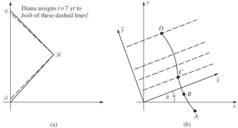
1.13 Appendix: The twin ‘paradox’ dissected 25
1.14 Exercises 28
2 Vector analysis in special relativity 33
2.1 Definition of a vector 33
2.2 Vector algebra 36
2.3 The four-velocity 41
2.4 The four-momentum 42
2.5 Scalar product 44
2.6 Applications 46
2.7 Photons 49
2.8 Further reading 50
2.9 Exercises 50
3 Tensor analysis in special relativity 56
3.1 The metric tensor 56
3.2 Definition of tensors 56
3.3 The01tensors: one-forms 58
viii Contents
t
3.5 Metric as a mapping of vectors into one-forms 68
3.6 Finally:MNtensors 72
3.7 Index ‘raising’ and ‘lowering’ 74
3.8 Differentiation of tensors 76
3.9 Further reading 77
3.10 Exercises 77
4 Perfect fluids in special relativity 84
4.1 Fluids 84
4.2 Dust: the number–flux vectorN 85
4.3 One-forms and surfaces 88
4.4 Dust again: the stress–energy tensor 91
4.5 General fluids 93
4.6 Perfect fluids 100
4.7 Importance for general relativity 104
4.8 Gauss’ law 105
4.9 Further reading 106
4.10 Exercises 107
5 Preface to curvature 111
5.1 On the relation of gravitation to curvature 111
5.2 Tensor algebra in polar coordinates 118
5.3 Tensor calculus in polar coordinates 125
5.4 Christoffel symbols and the metric 131
5.5 Noncoordinate bases 135
5.6 Looking ahead 138
5.7 Further reading 139
5.8 Exercises 139
6 Curved manifolds 142
6.1 Differentiable manifolds and tensors 142
6.2 Riemannian manifolds 144
6.3 Covariant differentiation 150
6.4 Parallel-transport, geodesics, and curvature 153
6.5 The curvature tensor 157
6.6 Bianchi identities: Ricci and Einstein tensors 163
6.7 Curvature in perspective 165
6.8 Further reading 166
6.9 Exercises 166
7 Physics in a curved spacetime 171
7.1 The transition from differential geometry to gravity 171
7.2 Physics in slightly curved spacetimes 175
ix Contents
t
7.4 Conserved quantities 178
7.5 Further reading 181
7.6 Exercises 181
8 The Einstein field equations 184
8.1 Purpose and justification of the field equations 184
8.2 Einstein’s equations 187
8.3 Einstein’s equations for weak gravitational fields 189
8.4 Newtonian gravitational fields 194
8.5 Further reading 197
8.6 Exercises 198
9 Gravitational radiation 203
9.1 The propagation of gravitational waves 203
9.2 The detection of gravitational waves 213
9.3 The generation of gravitational waves 227
9.4 The energy carried away by gravitational waves 234 9.5 Astrophysical sources of gravitational waves 242
9.6 Further reading 247
9.7 Exercises 248
10 Spherical solutions for stars 256
10.1 Coordinates for spherically symmetric spacetimes 256
10.2 Static spherically symmetric spacetimes 258
10.3 Static perfect fluid Einstein equations 260
10.4 The exterior geometry 262
10.5 The interior structure of the star 263
10.6 Exact interior solutions 266
10.7 Realistic stars and gravitational collapse 269
10.8 Further reading 276
10.9 Exercises 277
11 Schwarzschild geometry and black holes 281
11.1 Trajectories in the Schwarzschild spacetime 281
11.2 Nature of the surfacer=2M 298
11.3 General black holes 304
11.4 Real black holes in astronomy 318
11.5 Quantum mechanical emission of radiation by black holes:
the Hawking process 323
11.6 Further reading 327
11.7 Exercises 328
12 Cosmology 335
12.1 What is cosmology? 335
x Contents
t
12.3 Cosmological dynamics: understanding the expanding universe 353 12.4 Physical cosmology: the evolution of the universe we observe 361
12.5 Further reading 369
12.6 Exercises 370
Appendix A Summary of linear algebra 374
References 378
Preface to the second edition
In the 23 years between the first edition of this textbook and the present revision, the field of general relativity has blossomed and matured. Upon its solid mathematical foundations have grown a host of applications, some of which were not even imagined in 1985 when the first edition appeared. The study of general relativity has therefore moved from the periphery to the core of the education of a professional theoretical physicist, and more and more undergraduates expect to learn at least the basics of general relativity before they graduate.
My readers have been patient. Students have continued to use the first edition of this book to learn about the mathematical foundations of general relativity, even though it has become seriously out of date on applications such as the astrophysics of black holes, the detection of gravitational waves, and the exploration of the universe. This extensively revised second edition will, I hope, finally bring the book back into balance and give readers a consistent and unified introduction to modern research in classical gravitation.
The first eight chapters have seen little change. Recent references for further reading have been included, and a few sections have been expanded, but in general the geometrical approach to the mathematical foundations of the theory seems to have stood the test of time. By contrast, the final four chapters, which deal with general relativity in the astrophysical arena, have been updated, expanded, and in some cases completely re-written.
In Ch.9, on gravitational radiation, there is now an extensive discussion of detection with interferometers such as LIGO and the planned space-based detector LISA. I have also included a discussion of likely gravitational wave sources, and what we can expect to learn from detections. This is a field that is rapidly changing, and the first-ever direct detection could come at any time. Chapter9is intended to provide a durable framework for understanding the implications of these detections.
In Ch.10, the discussion of the structure of spherical stars remains robust, but I have inserted material on real neutron stars, which we see as pulsars and which are potential sources of detectable gravitational waves.
Chapter11, on black holes, has also gained extensive material about the astrophysical evidence for black holes, both for stellar-mass black holes and for the supermassive black holes that astronomers have astonishingly discovered in the centers of most galaxies. The discussion of the Hawking radiation has also been slightly amended.
Finally, Ch.12on cosmology is completely rewritten. In the first edition I essentially ignored the cosmological constant. In this I followed the prejudice of the time, which assumed that the expansion of the universe was slowing down, even though it had not yet been accurately enough measured. We now believe, from a variety of mutually consistent observations, that the expansion is accelerating. This is probably the biggest challenge to
xii Preface to the second edition
t
theoretical physics today, having an impact as great on fundamental theories of particle physics as on cosmological questions. I have organized Ch.12 around this perspective, developing mathematical models of an expanding universe that include the cosmological constant, then discussing in detail how astronomers measure the kinematics of the universe, and finally exploring the way that the physical constituents of the universe evolved after the Big Bang. The roles of inflation, of dark matter, and of dark energy all affect the structure of the universe today, and even our very existence. In this chapter it is possible only to give a brief taste of what astronomers have learned about these issues, but I hope it is enough to encourage readers to go on to learn more.
I have included more exercises in various chapters, where it was appropriate, but I have removed the exercise solutions from the book. They are available now on the website for the book.
The subject of this book remains classical general relativity; apart from a brief discussion of the Hawking radiation, there is no reference to quantization effects. While quantum gravity is one of the most active areas of research in theoretical physics today, there is still no clear direction to point a student who wants to learn how to quantize gravity. Perhaps by the third edition it will be possible to include a chapter on how gravity is quantized!
I want to thank many people who have helped me with this second edition. Several have generously supplied me with lists of misprints and errors in the first edition; I especially want to mention Frode Appel, Robert D’Alessandro, J. A. D. Ewart, Steve Fulling, Toshi Futamase, Ted Jacobson, Gerald Quinlan, and B. Sathyaprakash. Any remaining errors are, of course, my own responsibility. I thank also my editors at Cambridge University Press, Rufus Neal, Simon Capelin, and Lindsay Barnes, for their patience and encouragement. And of course I am deeply indebted to my wife Sian for her generous patience during all the hours, days, and weeks I spent working on this revision.
Preface to the first edition
This book has evolved from lecture notes for a full-year undergraduate course in general relativity which I taught from 1975 to 1980, an experience which firmly convinced me that general relativity is not significantly more difficult for undergraduates to learn than the standard undergraduate-level treatments of electromagnetism and quantum mechanics. The explosion of research interest in general relativity in the past 20 years, largely stimu-lated by astronomy, has not only led to a deeper and more complete understanding of the theory, it has also taught us simpler, more physical ways of understanding it. Relativity is now in the mainstream of physics and astronomy, so that no theoretical physicist can be regarded as broadly educated without some training in the subject. The formidable rep-utation relativity acquired in its early years (Interviewer: ‘Professor Eddington, is it true that only three people in the world understand Einstein’s theory?’ Eddington: ‘Who is the third?’) is today perhaps the chief obstacle that prevents it being more widely taught to theoretical physicists. The aim of this textbook is to present general relativity at a level appropriate for undergraduates, so that the student will understand the basic physical con-cepts and their experimental implications, will be able to solve elementary problems, and will be well prepared for the more advanced texts on the subject.
In pursuing this aim, I have tried to satisfy two competing criteria: first, to assume a min-imum of prerequisites; and, second, to avoid watering down the subject matter. Unlike most introductory texts, this one does not assume that the student has already studied electro-magnetism in its manifestly relativistic formulation, the theory of electromagnetic waves, or fluid dynamics. The necessary fluid dynamics is developed in the relevant chapters. The main consequence of not assuming a familiarity with electromagnetic waves is that grav-itational waves have to be introduced slowly: the wave equation is studied from scratch. A full list of prerequisites appears below.
The second guiding principle, that of not watering down the treatment, is very subjective and rather more difficult to describe. I have tried to introduce differential geometry fully, not being content to rely only on analogies with curved surfaces, but I have left out subjects that are not essential to general relativity at this level, such as nonmetric manifold theory, Lie derivatives, and fiber bundles.1 I have introduced the full nonlinear field equations, not just those of linearized theory, but I solve them only in the plane and spherical cases, quoting and examining, in addition, the Kerr solution. I study gravitational waves mainly in the linear approximation, but go slightly beyond it to derive the energy in the waves and the reaction effects in the wave emitter. I have tried in each topic to supply enough 1 The treatment here is therefore different in spirit from that in my bookGeometrical Methods of Mathematical
xiv Preface to the first edition
t
foundation for the student to be able to go to more advanced treatments without having to start over again at the beginning.
The first part of the book, up to Ch. 8, introduces the theory in a sequence that is typi-cal of many treatments: a review of special relativity, development of tensor analysis and continuum physics in special relativity, study of tensor calculus in curvilinear coordinates in Euclidean and Minkowski spaces, geometry of curved manifolds, physics in a curved spacetime, and finally the field equations. The remaining four chapters study a few top-ics that I have chosen because of their importance in modern astrophystop-ics. The chapter on gravitational radiation is more detailed than usual at this level because the observa-tion of gravitaobserva-tional waves may be one of the most significant developments in astronomy in the next decade. The chapter on spherical stars includes, besides the usual material, a useful family of exact compressible solutions due to Buchdahl. A long chapter on black holes studies in some detail the physical nature of the horizon, going as far as the Kruskal coordinates, then exploring the rotating (Kerr) black hole, and concluding with a simple discussion of the Hawking effect, the quantum mechanical emission of radiation by black holes. The concluding chapter on cosmology derives the homogeneous and isotropic met-rics and briefly studies the physics of cosmological observation and evolution. There is an appendix summarizing the linear algebra needed in the text, and another appendix contain-ing hints and solutions for selected exercises. One subject I have decided not to give as much prominence to, as have other texts traditionally, is experimental tests of general rel-ativity and of alternative theories of gravity. Points of contact with experiment are treated as they arise, but systematic discussions of tests now require whole books (Will 1981).2 Physicists today have far more confidence in the validity of general relativity than they had a decade or two ago, and I believe that an extensive discussion of alternative theories is therefore almost as out of place in a modern elementary text on gravity as it would be in one on electromagnetism.
The student is assumed already to have studied: special relativity, including the Lorentz transformation and relativistic mechanics; Euclidean vector calculus; ordinary and simple partial differential equations; thermodynamics and hydrostatics; Newtonian gravity (sim-ple stellar structure would be useful but not essential); and enough elementary quantum mechanics to know what a photon is.
The notation and conventions are essentially the same as in Misneret al., Gravitation (W. H. Freeman 1973), which may be regarded as one possible follow-on text after this one. The physical point of view and development of the subject are also inevitably influenced by that book, partly because Thorne was my teacher and partly becauseGravitationhas become such an influential text. But because I have tried to make the subject accessible to a much wider audience, the style and pedagogical method of the present book are very different.
Regarding the use of the book, it is designed to be studied sequentially as a whole, in a one-year course, but it can be shortened to accommodate a half-year course. Half-year courses probably should aim at restricted goals. For example, it would be reasonable to aim to teach gravitational waves and black holes in half a year to students who have already 2The revised second edition of this classic work is Will (1993).
xv Preface to the first edition
t
studied electromagnetic waves, by carefully skipping some of Chs. 1–3 and most of Chs. 4, 7, and 10. Students with preparation in special relativity and fluid dynamics could learn stellar structure and cosmology in half a year, provided they could go quickly through the first four chapters and then skip Chs. 9 and 11. A graduate-level course can, of course, go much more quickly, and it should be possible to cover the whole text in half a year.
Each chapter is followed by a set of exercises, which range from trivial ones (filling in missing steps in the body of the text, manipulating newly introduced mathematics) to advanced problems that considerably extend the discussion in the text. Some problems require programmable calculators or computers. I cannot overstress the importance of doing a selection of problems. The easy and medium-hard ones in the early chapters give essential practice, without which the later chapters will be much less comprehensible. The medium-hard and hard problems of the later chapters are a test of the student’s understand-ing. It is all too common in relativity for students to find the conceptual framework so interesting that they relegate problem solving to second place. Such a separation is false and dangerous: a student who can’t solve problems of reasonable difficulty doesn’t really understand the concepts of the theory either. There are generally more problems than one would expect a student to solve; several chapters have more than 30. The teacher will have to select them judiciously. Another rich source of problems is theProblem Book in Relativity and Gravitation, Lightmanet al.(Princeton University Press 1975).
I am indebted to many people for their help, direct and indirect, with this book. I would like especially to thank my undergraduates at University College, Cardiff, whose enthu-siasm for the subject and whose patience with the inadequacies of the early lecture notes encouraged me to turn them into a book. And I am certainly grateful to Suzanne Ball, Jane Owen, Margaret Vallender, Pranoat Priesmeyer, and Shirley Kemp for their patient typing and retyping of the successive drafts.
1
Special relativity
1.1 F u n d a m e n t a l p r i n c i p l e s o f s p e c i a l r e l a t i v i t y ( S R )
t h e o r y
The way in which special relativity is taught at an elementary undergraduate level – the level at which the reader is assumed competent – is usually close in spirit to the way it was first understood by physicists. This is an algebraic approach, based on the Lorentz transfor-mation (§1.7below). At this basic level, we learn how to use the Lorentz transformation to convert between one observer’s measurements and another’s, to verify and understand such remarkable phenomena as time dilation and Lorentz contraction, and to make elementary calculations of the conversion of mass into energy.
This purely algebraic point of view began to change, to widen, less than four years after Einstein proposed the theory.1Minkowski pointed out that it is very helpful to regard (t,x,y,z) as simply four coordinates in a four-dimensional space which we now call space-time. This was the beginning of the geometrical point of view, which led directly to general relativity in 1914–16. It is this geometrical point of view on special relativity which we must study before all else.
As we shall see, special relativity can be deduced from two fundamental postulates: (1) Principle of relativity(Galileo): No experiment can measure the absolute velocity of
an observer; the results of any experiment performed by an observer do not depend on his speed relative to other observers who are not involved in the experiment.
(2) Universality of the speed of light(Einstein): The speed of light relative to any unac-celerated observer isc=3×10⁸m s−1, regardless of the motion of the light’s source relative to the observer. Let us be quite clear about this postulate’s meaning: two differ-ent unaccelerated observers measuring the speed of thesame photonwill each find it to be moving at 3×10⁸m s−1relative to themselves, regardless of their state of motion relative to each other.
As noted above, the principle of relativity is not at all a modern concept; it goes back all the way to Galileo’s hypothesis that a body in a state of uniform motion remains in that state unless acted upon by some external agency. It is fully embodied in Newton’s second 1 Einstein’s original paper was published in 1905, while Minkowski’s discussion of the geometry of spacetime was given in 1908. Einstein’s and Minkowski’s papers are reprinted (in English translation) inThe Principle of Relativityby A. Einstein, H. A. Lorentz, H. Minkowski, and H. Weyl (Dover).
2 Special relativity
t
law, which contains only accelerations, not velocities themselves. Newton’s laws are, in fact, all invariant under the replacement
v(t)→v(t)=v(t)−V,
whereV is any constantvelocity. This equation says that a velocity v(t) relative to one observer becomesv(t) when measured by a second observer whose velocity relative to the first isV. This is called the Galilean law of addition of velocities.
By saying that Newton’s laws areinvariantunder the Galilean law of addition of veloc-ities, we are making a statement of a sort we will often make in our study of relativity, so it is well to start by making it very precise. Newton’s first law, that a body moves at a constant velocity in the absence of external forces, is unaffected by the replacement above, since ifv(t) is really a constant, sayv0, then the new velocityv0−Vis also a constant. Newton’s second law
F=ma=mdv/dt, is also unaffected, since
a−dv/dt=d(v−V)/dt=dv/dt=a.
Therefore, the second law will be valid according to the measurements of both observers, provided that we add to the Galilean transformation law the statement thatFandmare themselves invariant, i.e. the same regardless of which of the two observers measures them. Newton’s third law, that the force exerted by one body on another is equal and opposite to that exerted by the second on the first, is clearly unaffected by the change of observers, again because we assume the forces to be invariant.
So there is no absolute velocity. Is there an absolute acceleration? Newton argued that there was. Suppose, for example, that I am in a train on a perfectly smooth track,2eating a bowl of soup in the dining car. Then, if the train moves at constant speed, the soup remains level, thereby offering me no information about what my speed is. But, if the train changes its speed, then the soup climbs up one side of the bowl, and I can tell by looking at it how large and in what direction the acceleration is.3
Therefore, it is reasonable and useful to single out a class of preferred observers: those who are unaccelerated. They are calledinertial observers, and each one has a constant velocity with respect to any other one. These inertial observers are fundamental in spe-cial relativity, and when we use the term ‘observer’ from now on we will mean an inertial observer.
The postulate of the universality of the speed of light was Einstein’s great and radical contribution to relativity. It smashes the Galilean law of addition of velocities because it says that ifvhas magnitudec, then so doesv, regardless ofV. The earliest direct evidence for this postulate was the Michelson–Morely experiment, although it is not clear whether Einstein himself was influenced by it. The counter-intuitive predictions of special relativity all flow from this postulate, and they are amply confirmed by experiment. In fact it is probably fair to say that special relativity has a firmer experimental basis than any other of 2Physicists frequently have to make such idealizations, which often are far removed from common experience ! 3For Newton’s discussion of this point, see the excerpt from hisPrincipiain Williams (1968).
3 1.2 Definition of an inertial observer in SR
t
our laws of physics, since it is tested every day in all the giant particle accelerators, which send particles nearly to the speed of light.
Although the concept of relativity is old, it is customary to refer to Einstein’s theory sim-ply as ‘relativity’. The adjective ‘special’ is applied in order to distinguish it from Einstein’s theory of gravitation, which acquired the name ‘general relativity’ because it permits us to describe physics from the point of view of both accelerated and inertial observers and is in that respect a more general form of relativity. But the real physical distinction between these two theories is that special relativity (SR) is capable of describing physics only in the absence of gravitational fields, while general relativity (GR) extends SR to describe gravitation itself.4 We can only wish that an earlier generation of physicists had chosen more appropriate names for these theories !
1.2 D e f i n i t i o n o f a n i n e r t i a l o b s e r v e r i n S R
It is important to realize that an ‘observer’ is in fact a huge information-gathering system, not simply one man with binoculars. In fact, we shall remove the human element entirely from our definition, and say that an inertial observer is simply a coordinate system for spacetime, which makes an observation simply by recording the location (x,y,z) and time (t) of any event. This coordinate system must satisfy the following three properties to be calledinertial:
(1) The distance between point P1 (coordinates x1,y1,z1) and point P2 (coordinates x2,y2,z2) is independent of time.
(2) The clocks that sit at every point ticking off the time coordinatetare synchronized and all run at the same rate.
(3) The geometry of space at any constant timetis Euclidean.
Notice that this definition does not mention whether the observer accelerates or not. That will come later. It will turn out that only an unaccelerated observer can keep his clocks synchronized. But we prefer to start out with this geometrical definition of an inertial observer. It is a matter for experiment to decide whether such an observer can exist: it is not self-evident that any of these propertiesmustbe realizable, although we would probably expect a ‘nice’ universe to permit them! However, we will see later in the course that a gravitational field does generally make it impossible to construct such a coordinate system, and this is why GR is required. But let us not get ahead of the story. At the moment we are assuming that we canconstruct such a coordinate system (that, if you like, the gravitational fields around us are so weak that they do not really matter). We can envision this coordinate system, rather fancifully, as a lattice of rigid rods filling space, with a clock at every intersection of the rods. Some convenient system, such as a collection of GPS 4 It is easy to see that gravitational fields cause problems for SR. If an astronaut in orbit about Earth holds a bowl of soup, does the soup climb up the side of the bowl in response to the gravitational ‘force’ that holds the spacecraft in orbit? Two astronauts in different orbits accelerate relative to one another, but neitherfeels
an acceleration. Problems like this make gravity special, and we will have to wait until Ch.5to resolve them. Until then, the word ‘force’ will refer to a nongravitational force.
4 Special relativity
t
satellites and receivers, is used to ensure that all the clocks are synchronized. The clocks are supposed to be very densely spaced, so that there is a clock next to every event of interest, ready to record its time of occurrence without any delay. We shall now define how we use this coordinate system to make observations.
Anobservationmade by the inertial observer is the act of assigning to any event the coordinates x,y,z of the location of its occurrence, and the time read by the clock at (x,y,z) when the event occurred. It isnotthe timeton the wrist watch worn by a scientist located at (0, 0, 0) when he first learns of the event. Avisualobservation is of this second type: the eye regards as simultaneous all events itseesat the same time; an inertial observer regards as simultaneous all events thatoccurat the same time as recorded by the clock nearest them when the events occurred. This distinction is important and must be borne in mind. Sometimes we will say ‘an observer sees. . .’ but this will only be shorthand for ‘measures’. We will never mean avisualobservation unless we say so explicitly.
An inertial observer is also called an inertial reference frame, which we will often abbreviate to ‘reference frame’ or simply ‘frame’.
1.3 N e w u n i t s
Since the speed of lightcis so fundamental, we shall from now on adopt a new system of units for measurements in whichcsimply has the value 1! It is perfectly okay for slow-moving creatures like engineers to be content with the SI units: m, s, kg. But it seems silly in SR to use units in which the fundamental constantchas the ridiculous value 3×10⁸. The SI units evolved historically. Meters and seconds are not fundamental; they are simply convenient for human use. What we shall now do is adopt a new unit for time, the meter. One meter of time is the time it takes light to travel one meter. (You are probably more familiar with an alternative approach: a year of distance – called a ‘light year’ – is the distance light travels in one year.) The speed of light in these units is:
c=distance light travels in any given time interval the given time interval
= 1 m
the time it takes light to travel one meter
=1 m
1 m =1.
So if we consistently measure time in meters, thencis not merely 1, it is also dimension-less! In converting from SI units to these ‘natural’ units, we can use any of the following relations:
3×10⁸m s−1=1,
1 s=3×10⁸m, 1 m= 1
5 1.4 Spacetime diagrams
t
The SI units contain many ‘derived’ units, such as joules and newtons, which are defined in terms of the basic three: m, s, kg. By converting from s to m these units simplify consid-erably: energy and momentum are measured in kg, acceleration in m−1, force in kg m−1, etc. Do the exercises on this. With practice, these units will seem as natural to you as they do to most modern theoretical physicists.
1.4 S p a c e t i m e d i a g r a m s
A very important part of learning the geometrical approach to SR is mastering the space-time diagram. In the rest of this chapter we will derive SR from its postulates by using spacetime diagrams, because they provide a very powerful guide for threading our way among the many pitfalls SR presents to the beginner. Fig. 1.1 below shows a two-dimensional slice of spacetime, thet−xplane, in which are illustrated the basic concepts. A single point in this space5 is a point of fixedx and fixedt, and is called anevent. A line in the space gives a relation x=x(t), and so can represent the position of a parti-cle at different times. This is called the partiparti-cle’s world line. Its slope is related to its velocity,
slope=dt/dx=1/v.
Notice that a light ray (photon) always travels on a 45◦line in this diagram.
x (m)
t
(m)
Accelerated world line
World line of light, v=1 World line of particle moving at speed |v|<1
World line with velocity
v>1 An event
t
Figure 1.1 A spacetime diagram in natural units.5 We use the word ‘space’ in a more general way than you may be used to. We do not mean a Euclidean space in which Euclidean distances are necessarily physically meaningful. Rather, we mean just that it is a set of points that is continuous (rather than discrete, as a lattice is). This is the first example of what we will define in Ch.5 to be a ‘manifold’.
6 Special relativity
t
We shall adopt the following notational conventions:
(1) Events will be denoted by cursive capitals, e.g. A,B,P. However, the letter O is reserved to denote observers.
(2) The coordinates will be called (t,x,y,z). Any quadruple of numbers like (5,−3, 2, 1016) denotes an event whose coordinates are t=5, x= −3,y=2, z=1016. Thus, we always puttfirst. All coordinates are measured in meters.
(3) It is often convenient to refer to the coordinates (t,x,y,z) as a whole, or to each indifferently. That is why we give them thealternative names(x0,x1,x2,x3). These superscripts arenotexponents, but just labels, called indices. Thus (x3)2denotes the square of coordinate 3 (which isz), not the square of the cube ofx.Generically, the coordinatesx0,x1,x2, andx3are referred to asxα. AGreek index(e.g.α,β,μ,ν) will be assumed to take a value from the set (0, 1, 2, 3). Ifαis not given a value, thenxα is anyof the four coordinates.
(4) There are occasions when we want to distinguish between t on the one hand and (x,y,z) on the other. We use Latin indicesto refer to the spatial coordinates alone. Thus a Latin index (e.g.a,b,i,j,k,l) will be assumed to take a value from the set (1, 2, 3). Ifiis not given a value, thenxiisanyof the three spatial coordinates. Our conventions on the use of Greek and Latin indices are by no means universally used by physicists. Some books reverse them, using Latin for{0, 1, 2, 3}and Greek for{1, 2, 3}; others usea,b,c,. . .for one set andi,j,kfor the other. Students should always check the conventions used in the work they are reading.
1.5 C o n s t r u c t i o n o f t h e c o o r d i n a t e s u s e d b y
a n o t h e r o b s e r v e r
Since any observer is simply a coordinate system for spacetime, and since all observers look at the same events (the same spacetime), it should be possible to draw the coordinate lines of one observer on the spacetime diagram drawn by another observer. To do this we have to make use of the postulates of SR.
Suppose an observerOuses the coordinatest,xas above, and that another observerO¯, with coordinates¯t,x¯, is moving with velocityvin thexdirection relative toO. Where do the coordinate axes for¯tandx¯go in the spacetime diagram ofO?
¯t axis: This is the locus of events at constantx¯=0 (andy¯= ¯z=0, too, but we shall ignore them here), which is the locus of the origin ofO¯’s spatial coordinates. This isO¯’s world line, and it looks like that shown in Fig.1.2.
¯
x axis: To locate this we make a construction designed to determine the locus of events at¯t=0, i.e. those thatO¯ measures to be simultaneous with the event¯t= ¯x=0.
Consider the picture inO¯’s spacetime diagram, shown in Fig.1.3. The events on thex¯ axis all have the following property: A light ray emitted at eventEfromx¯=0 at, say, time
¯t= −awill reach thex¯axis atx¯=a(we call this eventP); if reflected, it will return to the pointx¯=0 at¯t= +a, called eventR. Thex¯axis can bedefined, therefore, as the locus of
7 1.5 Construction of the coordinates used by another observer
t
t
t
x
Tangent of this angle isυ
t
Figure 1.2 The time-axis of a frame whose velocity isv.t
x
a
a
–a
t
Figure 1.3 Light reflected ata, as measured byO¯.events that reflect light rays in such a manner that they return to the¯taxis at+aif they left it at−a, for anya. Now look at this in the spacetime diagram ofO, Fig.1.4.
We know where the¯taxis lies, since we constructed it in Fig.1.2. The events of emis-sion and reception,¯t= −aand¯t= +a, are shown in Fig.1.4. Sinceais arbitrary, it does not matter where along the negative¯t axis we place eventE, so no assumption need yet be made about the calibration of the¯taxis relative to thetaxis. All that matters for the moment is that the eventRon the¯taxis must be as far from the origin as eventE. Having drawn them in Fig.1.4, we next draw in the same light beam as before, emitted fromE, and traveling on a 45◦ line in this diagram. The reflected light beam must arrive atR, so it is the 45◦ line with negative slope throughR. The intersection of these two light beams must be the event of reflection P. This establishes the location ofP in our dia-gram. The line joining it with the origin – the dashed line – must be thex¯ axis: it does
8 Special relativity
t
t
a
x
–a
t
x
t
Figure 1.4 The reflection in Fig.1.3, as measuredO.t
φ φ
x
x t
(a)
t
φ
φ x
x t
(b)
t
Figure 1.5 Spacetime diagrams ofO(left) andO¯ (right).not coincide with the xaxis. If you compare this diagram with the previous one, you will see why: in both diagrams light moves on a 45◦line, while thetand¯taxes change slope from one diagram to the other. This is the embodiment of the second fundamental postulate of SR: that the light beam in question has speedc=1 (and hence slope=1) with respect toeveryobserver. When we apply this to these geometrical constructions we immediately find that the events simultaneous toO¯(the line¯t=0, hisxaxis) are not simul-taneous toO(are not parallel to the linet=0, thexaxis). Thisfailure of simultaneityis inescapable.
The following diagrams (Fig.1.5) represent the same physical situation. The one on the left is the spacetime diagramO, in whichO¯ moves to the right. The one on the right is drawn from the point of view ofO¯, in whichOmoves to the left. The four angles are all equal to arc tan|v|, where|v|is the relative speed ofOandO¯.
9 1.6 Invariance of the interval
t
1.6 I n v a r i a n c e o f t h e i n t e r v a l
We have, of course, not quite finished the construction of O¯’s coordinates. We have the position of his axes but not the length scale along them. We shall find this scale by proving what is probably the most important theorem of SR, the invariance of the interval.
Consider two events on the world line of the same light beam, such as E and P in Fig. 1.4. The differences (t,x,y,z) between the coordinates of E and P in some frame O satisfy the relation (x)2+(y)2+(z)2−(t)2=0, since the speed of light is 1. But by the universality of the speed of light, the coordinate differences between the same two events in the coordinates of O¯(¯t,x¯,¯y,¯z) also satisfy (x¯)2+(¯y)2+(¯z)2−(¯t)2=0. We shall define theintervalbetweenanytwo events (not necessarily on the same light beam’s world line) that are separated by coordinate increments (t,x,y,z) to be6
s2= −
(t)2+(x)2+(y)2+(z)2. (1.1)
It follows that ifs2=0 for two events using their coordinates inO, thens¯2=0 for the same two events using their coordinates inO¯. What does this imply about the relation between the coordinates of the two frames? To answer this question, we shall assume that the relation between the coordinates ofOandO¯ islinearand that we choose their origins to coincide (i.e. that the events¯t= ¯x= ¯y= ¯z=0 andt=x=y=z=0 are the same). Then in the expression for¯s2,
s¯2= −(¯t)2+(x¯)2+(y¯)2+(z¯)2,
the numbers (¯t,x¯,y¯,¯z) are linear combinations of their unbarred counterparts, which means thats¯2is aquadraticfunction of the unbarred coordinate increments. We can therefore write
¯s2= 3
α=0 3
β=0
Mαβ(xα)(xβ) (1.2) for some numbers {Mαβ;α,β=0,. . ., 3}, which may be functions of v, the relative velocity of the two frames. Note that we can suppose thatMαβ=Mβα for allαandβ, since only the sum Mαβ+Mβα ever appears in Eq. (1.2) when α=β. Now we again suppose thats2=0, so that from Eq. (1.1) we have
t=r, r=[(x)2+(y)2+(z)2]1/2.
6 The student to whom this is new should probably regard the notations2as a single symbol, not as the square of a quantitys. Sinces2can be either positive or negative, it is not convenient to take its square root. Some authors do, however, calls2the ‘squared interval’, reserving the name ‘interval’ fors=√(s2). Note also that the notations2nevermeans(s2).
10 Special relativity
t
(We have supposedt>0 for convenience.) Putting this into Eq. (1.2) gives s¯2=M00(r)2+2
3
i=1
M0ixi
r
+
3
i=1 3
j=1
Mijxixj. (1.3)
But we have already observed thats¯2must vanish ifs2does, and this must be true for arbitrary{xi,i=1, 2, 3}. It is easy to show (see Exer. 8, §1.14) that this implies
M0i=0 i=1, 2, 3 (1.4a)
and
Mij= −(M00)δij (i,j=1, 2, 3), (1.4b)
whereδijis the Kronecker delta, defined by
δij =
1 ifi=j,
0 ifi=j. (1.4c)
From this and Eq. (1.2) we conclude that
¯s2=M00[(t)2−(x)2−(y)2−(z)2]. If we define a function
φ(v)= −M00,
then we have proved the following theorem:The universality of the speed of light implies that the intervalss2ands¯2between any two events as computed by different observers satisfy the relation
¯s2=φ(v)s2. (1.5)
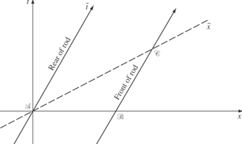
We shall now show that, in fact,φ(v)=1, which is the statement that the interval is independent of the observer. The proof of this has two parts. The first part shows thatφ(v) depends only on|v|. Consider a rod which is oriented perpendicular to the velocityvofO¯ relative toO. Suppose the rod is at rest inO, lying on theyaxis. In the spacetime diagram ofO(Fig.1.6), the world lines of its ends are drawn and the region between shaded. It is easy to see that the square of its length is just the interval between the two eventsAandB that are simultaneous inO(att=0) and occur at the ends of the rod. This is because, for these events, (x)AB=(z)AB=(t)AB=0. Now comes the key point of the first part of the proof: the eventsAandBare simultaneous as measured byO¯ as well. The reason is most easily seen by the construction shown in Fig.1.7, which is the same spacetime diagram as Fig.1.6, but in which the world line of a clock in O¯ is drawn. This line is perpendicular to theyaxis and parallel to thet−xplane, i.e. parallel to the¯taxis shown in Fig.1.5(a).
Suppose this clock emits light rays at eventP which reach eventsAandB. (Not every clock can do this, so we have chosen the one clock inO¯ which passes through theyaxis
11 1.6 Invariance of the interval
t
World lines of ends of rod
t
x
y
t
Figure 1.6 A rod at rest inO, lying on they-axis.t
x
y
Clock in
t
Figure 1.7 A clock ofO¯’s frame, moving in thex-direction inO’s frame.att=0 and can send out such light rays.) The light rays reflect fromAandB, and we can see from the geometry (if you can allow for the perspective in the diagram) that they arrive back atO¯’s clock at thesameeventL. Therefore, fromO¯’s point of view, the two events occur at the same time. (This is thesameconstruction we used to determine thex¯axis.) But ifAandBare simultaneous inO¯, then the interval between them inO¯ is also the square of their length inO¯. The result is:
(length of rod inO¯)2=φ(v)(length of rod inO)2.
On the other hand, the length of the rod cannot depend on thedirection of the velocity, because the rod is perpendicular to it and there are no preferred directions of motion (the principle of relativity). Hence the first part of the proof concludes that
12 Special relativity
t
The second step of the proof is easier. It uses the principle of relativity to show that φ(|v|)=1. Consider three frames,O,O¯, andO. FrameO¯ moves with speedvin, say, the xdirection relative toO. FrameOmoves with speedvin the negativexdirection relative toO¯. It is clear thatO is in fact identical toO, but for the sake of clarity we shall keep separate notation for the moment. We have, from Eqs. (1.5) and (1.6),
s2=φ(v)¯s2 s¯2=φ(v)s2
⇒s2=[φ(v)]2s2. But sinceOandOare identical,s2ands2are equal. It follows that
φ(v)= ±1.
We must choose the plus sign, since in the first part of this proof the square of the length of a rod must be positive. We have, therefore, proved the fundamental theorem thatthe interval between any two events is the same when calculated by any inertial observer:
¯s2=s2. (1.7)
Notice that from the first part of this proof we can also conclude now thatthe length of a rod oriented perpendicular to the relative velocity of two frames is the same when measured by either frame. It is also worth reiterating that the construction in Fig.1.7proved a related result, thattwo events which are simultaneous in one frame are simultaneous in any frame moving in a direction perpendicular to their separation relative to the first frame.
Becauses2is a property only of the two events and not of the observer, it can be used to classify the relation between the events. Ifs2is positive (so that the spatial increments dominatet), the events are said to bespacelike separated. Ifs2is negative, the events are said to betimelike separated. Ifs2is zero (so the events are on the same light path), the events are said to belightlikeornull separated.
t
x
y
13 1.6 Invariance of the interval
t
The events that are lightlike separated from any particular eventA, lie on a cone whose apex isA. This cone is illustrated in Fig.1.8. This is called thelight cone ofA. All events within the light cone are timelike separated from A; all events outside it are spacelike separated. Therefore, all events inside the cone can be reached fromA on a world line which everywhere moves in a timelike direction. Since we will see later that nothing can move faster than light, all world lines of physical objects move in a timelike direc-tion. Therefore, events inside the light cone are reachable from Aby a physical object, whereas those outside are not. For this reason, the events inside the ‘future’ or ‘forward’ light cone are sometimes called theabsolute futureof the apex; those within the ‘past’ or ‘backward’ light cone are called theabsolute past; and those outside are called the abso-lute elsewhere. The events on the cone are therefore the boundary of the absolute past
Galileo:
Einstein:
Two events:
t
t
t
Future of event
Past of event
Past of ‘Elsewhere’
of ‘Elsewhere’ of Future of
Common future
Future of Future
of
Past of Past of
x
x
x
‘Now’ for event
‘Now’ is only
itself
Common past
14 Special relativity
t
and future. Thus, although ‘time’ and ‘space’ can in some sense be transformed into one another in SR, it is important to realize that we can still talk about ‘future’ and ‘past’ in an invariant manner. To Galileo and Newton the past was everything ‘earlier’ than now; all of spacetime was the union of the past and the future, whose boundary was ‘now’. In SR, the past is only everything inside the past light cone, and spacetime hasthree invari-ant divisions: SR adds the notion of ‘elsewhere’. What is more, althoughall observers agree on what constitutes the past, future, and elsewhere of a given event (because the interval is invariant), each different event has adifferent past and future; no two events have identical pasts and futures, even though they can overlap. These ideas are illustrated in Fig.1.9.
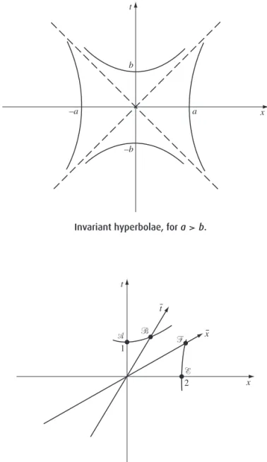
1.7 I n v a r i a n t h y p e r b o l a e
We can now calibrate the axes ofO¯’s coordinates in the spacetime diagram ofO, Fig.1.5. We restrict ourselves to thet−xplane. Consider a curve with the equation
−t2+x2=a2,
where a is a real constant. This is a hyperbola in the spacetime diagram of O, and it passes through all events whose interval from the origin isa2. By the invariance of the interval, these same events have intervala2from the origin inO¯, so they also lie on the curve−¯t2+ ¯x2=a2. This is a hyperbola spacelike separated from the origin. Similarly, the events on the curve
−t2+x2= −b2
all have timelike interval−b2from the origin, and also lie on the curve−¯t2+ ¯x2= −b2. These hyperbolae are drawn in Fig.1.10. They are all asymptotic to the lines with slope
±1, which are of course the light paths through the origin. In a three-dimensional diagram (in which we add theyaxis, as in Fig.1.8), hyperbolae of revolution would be asymptotic to the light cone.
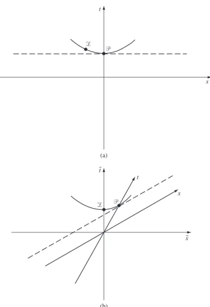
We can now calibrate the axes ofO¯. In Fig.1.11the axes ofOandO¯ are drawn, along with an invariant hyperbola of timelike interval−1 from the origin. EventAis on thet axis, so hasx=0. Since the hyperbola has the equation
−t2+x2= −1,
it follows that eventAhast=1. Similarly, eventBlies on the¯taxis, so has¯x=0. Since the hyperbola also has the equation
−¯t2+ ¯x2= −1,
it follows that eventBhas¯t=1. We have, therefore, used the hyperbolae to calibrate the¯t axis. In the same way, the invariant hyperbola
15 1.7 Invariant hyperbolae
t
b
–a
–b
a x
t
t
Figure 1.10 Invariant hyperbolae, fora>b.
t
x
1
2
t
x
t
Figure 1.11 Using the hyperbolae through eventsAandEto calibrate thex¯and¯taxes.
shows that eventE has coordinatest=0,x=2 and that eventF has coordinates¯t=0,
¯
x=2. This kind of hyperbola calibrates the spatial axes ofO¯.
Notice that event B looks to be ‘further’ from the origin than A. This again shows the inappropriateness of using geometrical intuition based upon Euclidean geometry. Here the important physical quantity is the interval−(t)2+(x)2, not the Euclidean distance (t)2+(x)2. The student of relativity has to learn to uses2as the physical measure of ‘distance’ in spacetime, and he has to adapt his intuition accordingly. This is not, of course, in conflict with everyday experience. Everyday experience asserts that ‘space’ (e.g. the
16 Special relativity
t
section of spacetime witht=0) is Euclidean. For events that havet=0 (simultaneous to observerO), the interval is
s2=(x)2+(y)2+(z)2.
This is just their Euclidean distance. The new feature of SR is that time can (and must) be brought into the computation of distance. It is not possible to define ‘space’ uniquely since different observers identify different sets of events to be simultaneous (Fig.1.5). But there is still a distinction between space and time, since temporal increments enters2 with the opposite sign from spatial ones.
t
x x t
x t
(b) (a)
t
Figure 1.12 (a) A line of simultaneity inOis tangent to the hyperbola atP. (b) The same tangency as seen byO¯.
17 1.8 Particularly important results
t
In order to use the hyperbolae to derive the effects of time dilation and Lorentz contrac-tion, as we do in the next seccontrac-tion, we must point out a simple but important property of the tangent to the hyperbolae.
In Fig.1.12(a) we have drawn a hyperbola and its tangent atx=0, which is obviously a line of simultaneityt=const. In Fig.1.12(b) we have drawn the same curves from the point of view of observer O¯ who moves to the left relative toO. The eventP has been shifted to the right: it could be shifted anywhere on the hyperbola by choosing the Lorentz transformation properly. The lesson of Fig.1.12(b) is that the tangent to a hyperbola at any eventPis a line of simultaneity of the Lorentz frame whose time axis joinsPto the origin. If this frame has velocityv, the tangent has slopev.
1.8 P a r t i c u l a r l y i m p o r t a n t r e s u l t s
Time dilation
From Fig.1.11and the calculation following it, we deduce that when a clock moving on the
¯
taxis reachesBit has a reading of¯t=1, but that eventBhas coordinatet=1/√(1−v2) inO. So toOit appears to run slowly:
(t)measured inO =(¯t√)measured inO¯
(1−v2) . (1.8)
Notice that¯tis the time actually measured by a single clock, which moves on a world line from the origin toB, whiletis the difference in the readings of two clocks at rest inO; one on a world line through the origin and one on a world line throughB. We shall return to this observation later. For now, we define theproper timebetween eventsBand the origin to be the time ticked off by a clock which actually passes through both events. It is a directly measurable quantity, and it is closely related to the interval. Let the clock be at rest in frameO¯, so that the proper timeτ is the same as the coordinate time¯t. Then, since the clock is at rest inO¯, we havex¯=y¯=z¯=0, so
s2= −¯
t2= −τ2. (1.9)
The proper time is just the square root of the negative of the interval. By expressing the interval in terms ofO’s coordinates we get
τ =[(t)2−(x)2−(y)2−(z)2]1/2
=t√(1−v2). (1.10)
18 Special relativity
t
t
x
x t
Rear of rod
Front of rod
t
Figure 1.13 The proper length ofACis the length of the rod in its rest frame, while that ofABis its length inO.
Lorentz contraction
In Fig.1.13we show the world path of a rod at rest inO¯. Its length inO¯ is the square root ofs2AC, while its length inOis the square root ofs2AB. If eventChas coordinates
¯t=0,x¯=l, then by the identical calculation from before it hasxcoordinate inO xC=l/√(1−v2),
and since thex¯axis is the linet=vx, we have
tC=vl/√(1−v2). The lineBChas slope (relative to thet-axis)
x/t=v, and so we have
xC−xB tC−tB =v, and we want to knowxB whentB=0. Thus,
xB=xC−vtC
= √ l
(1−v2)− v2l
√
(1−v2) =l
√
(1−v2). (1.11) This is the Lorentz contraction.
Conventions
The interval s2 is one of the most important mathematical concepts of SR but there is no universal agreement on its definition: many authors defines2=(t)2−(x)2−
19 1.8 Particularly important results
t
(y)2−(z)2. This overall sign is a matter of convention (like the use of Latin and Greek indices we referred to earlier), since invariance ofs2implies invariance of −s2. The physical result of importance is just this invariance, which arises from the difference in sign between the (t)2 and [(x)2+(y)2+(z)2] parts. As with other conventions, students should ensure they know which sign is being used: it affects all sorts of formulae, for example Eq. (1.9).
Failure of relativity?
Newcomers to SR, and others who don’t understand it well enough, often worry at this point that the theory is inconsistent. We began by assuming the principle of relativity, which asserts that all observers are equivalent. Now we have shown that ifO¯ moves relative toO, the clocks ofO¯will be measured byOto be running more slowly than those ofO. So isn’t it therefore the case thatO¯ will measureO’s clocks to be running faster than his own? If so, this violates the principle of relativity, since we could as easily have begun withO¯ and deduced thatO’s clocks run more slowly thanO¯’s.
This is what is known as a ‘paradox’, but like all ‘paradoxes’ in SR, this comes from not having reasoned correctly. We will now demonstrate, using spacetime diagrams, that
¯
O measuresO’s clocks to be running more slowly. Clearly, we could simply draw the spacetime diagram fromO¯’s point of view, and the result would follow. But it is more instructive to stay inO’s spacetime diagram.
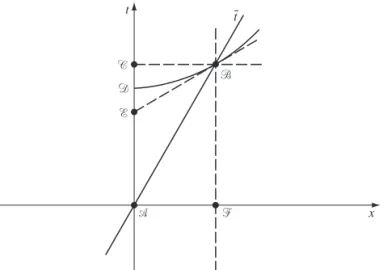
Different observers will agree on the outcome of certain kinds of experiments. For exam-ple, ifAflips a coin,everyobserver will agree on the result. Similarly, if two clocks are right next to each other, all observers will agree which is reading an earlier time than the other. But the question of therateat which clocks run can only be settled by comparing the same two clocks on two different occasions, and if the clocks are moving relative to one another, then they can be next to each other on only one of these occasions. On the other occasion they must be compared over some distance, and different observers may draw different conclusions. The reason for this is that they actually perform different and inequivalent experiments. In the following analysis, we will see that each observer usestwo of his own clocks and one of the other’s. This asymmetry in the ‘design’ of the experiment gives the asymmetric result.
Let us analyzeO’s measurement first, in Fig.1.14. This consists of comparing the read-ing on a sread-ingle clock ofO¯ (which travels fromAtoB) with twoclocks of his own: the first is the clock at the origin, which readsO¯’s clock at eventA; and the second is the clock which is atF att=0 and coincides withO¯’s clock atB. This second clock ofO moves parallel to the first one, on the vertical dashed line. WhatOsays is that both clocks atAreadt=0, while atBthe clock ofO¯ reads¯t=1, while that ofOreads a later time, t=(1−v2)−1/2. Clearly,O¯ agrees with this, as he is just as capable of looking at clock dials asOis. But forOto claim thatO¯’s clock is running slowly, he must be sure that his own two clocks are synchronized, for otherwise there is no particular significance in observing that atBthe clock ofO¯lags behind that ofO. Now, fromO’s point of view, his
20 Special relativity
t
t t
x
t
Figure 1.14 The proper length ofABis the time ticked by a clock at rest inO¯, while that ofACis the time it takes to do so as measured byO.
clocksaresynchronized, and the measurement and its conclusion are valid. Indeed, they are the only conclusions he can properly make.
ButO¯need not accept them, because to himO’s clocks arenotsynchronized. The dotted line throughBis the locus of events thatO¯ regards as simultaneous toB. EventEis on this line, and is the tick ofO’s first clock, whichO¯measures to be simultaneous with eventB. A simple calculation shows this to be att=(1−v2)1/2, earlier thanO’s other clock atB, which is reading (1−v2)−1/2. SoO¯ can rejectO’s measurement since the clocks involved aren’t synchronized. Moreover, ifO¯studiesO’s first clock, he concludes that it ticks from t=0 tot=(1−v2)1/2(i.e. fromAtoB) in the time it takes his own clock to tick from
¯t=0 to¯t=1 (i.e. fromAtoB). So he regardsO’s clocks as running more slowly than his own.
It follows that the principle of relativity is not contradicted: each observer measures the other’s clock to be running slowly. The reason they seem to disagree is that they measure different things. ObserverOcompares the interval fromAtoBwith that fromAtoC. The other observer compares that fromAtoBwith that fromAtoE. All observers agree on the values of the intervals involved. What they disagree on is which pair to use in order to decide on the rate at which a clock is running. This disagreement arises directly from the fact that the observers do not agree on which events are simultaneous. And, to reiterate a point that needs to be understood, simultaneity (clock synchronization) is at the heart of clock comparisons:Ousestwoof his clocks to ‘time’ the rate ofO¯’s one clock, whereas
¯
Ouses two of his own clocks to time one clock ofO.
Is this disagreement worrisome? It should not be, but it should make the student very cautious. The fact that different observers disagree on clock rates or simultaneity just means that such concepts are not invariant: they are coordinate dependent. It doesnotprevent any given observer from using such concepts consistently himself. For example,Ocan say that
AandFare simultaneous, and he is correct in the sense that they have the same value of the coordinatet. For him this is a useful thing to know, as it helps locate the events in spacetime.