False Discovery Rate Control with Groups

False Discovery Rate Control with Groups

James X. Hu, Hongyu Zhao and Harrison H. Zhou

Abstract

In the context of large-scale multiple hypothesis testing, the hypotheses often possess certain group structures based on additional information such as Gene On-tology in gene expression data and phenotypes in genome-wide association studies. It is hence desirable to incorporate such information when dealing with multiplicity problems to increase statistical power. In this article, we demonstrate the benefit of considering group structure by presenting a p-value weighting procedure which utilizes the relative importance of each group while controlling the false discovery rate under weak conditions. The procedure is easy to implement and shown to be more powerful than the classical Benjamini-Hochberg procedure in both theoretical and simulation studies. By estimating the proportion of true null hypotheses, the data-driven procedure controls the false discovery rate asymptotically. Our analy-sis on one breast cancer data set confirms that the procedure performs favorably ∗_{James X. Hu is Ph.D candidate, Department of Statistics, Yale University, New Haven, CT 06511.}

(Email:[email protected]). Hongyu Zhao is Professor of Biostatistics Division, Department of Epidemiol-ogy and Public Health, Yale University, New Haven, CT 06511 (Email:[email protected]). Harrison H. Zhou is Assistant Professor, Department of Statistics, Yale University, New Haven, CT 06511 (Email:

[email protected]). James Hu and Harrison Zhou’s research is supported in part by NSF Grant DMS-0645676. Hongyu Zhao’s research is supported in part by NSF grant DMS-0714817 and NIH grant GM59507.

compared with the classical method.

Key Words: False discovery rate; group structure; Benjamini-Hochberg proce-dure; positive regression dependence; adaptive procedure.

1

INTRODUCTION

Ever since the seminal work of Benjamini and Hochberg (1995), the concept of false dis-covery rate (FDR) and the FDR controlling Benjamini-Hochberg (BH) procedure have been widely adopted to replace traditional methods, like family-wise error rate (FWER), in fields such as bioinformatics where a large number of hypotheses are tested. For exam-ple, in gene expression microarray experiments or brain image studies, each gene or brain location is associated with one hypothesis. Usually there are tens of thousands of them. The more conservative family-wise error rate controlling procedures often have extremely low power as the number of hypotheses gets large. Under the FDR framework, the power can be increased.

In many cases, there is prior information that a natural group structure exists among the hypotheses, or the hypotheses can be divided into subgroups based on the character-istics of the problem. For example, for gene expression data, Gene Ontology (The Gene Ontology Consortium2000) provides a natural stratification among genes based on three ontologies. In genome-wide association study, each marker might be tested for associa-tion with several phenotypes of interest; or tests might be conducted assuming different genetic models (Sun, Craiu, Paterson and Bull, 2006). In clinical trials, hypotheses are commonly divided into primary and secondary based on the relative importance of the features of the disease (Dmitrienko, Offen and Westfall, 2003). Ignorance of such group

structures in data analysis can be dangerous. Efron (2008) pointed out that applying multiple comparison treatments such as FDR to the entire set of hypotheses may lead to overly conservative or overly liberal conclusions within any particular subgroup of the cases.

In multiple hypothesis testing, utilizing group structure can be achieved by assigning weights for the hypotheses (or p-values) in each group. Such an idea of using group in-formation and weights has been adopted by several authors. Efron (2008) considered the Separate-Class model where the hypotheses are divided into distinct groups, and showed the legitimacy of such separate analysis for FDR methods. Benjamini and Hochberg (1997) analyzed both the p-value weighting and the error weighting methods and evalu-ated different procedures. Genovese, Roeder and Wasserman (2006) investigevalu-ated the merit of multiple testing procedures using weighted p-values and claimed that their weighted Benjamini-Hochberg procedure controls the FWER and FDR while improving power. Wasserman and Roeder (2006) further explored theirp-value weighting procedure by in-troducing an optimal weighting scheme for FWER control. Roeder, Bacanu, Wasserman and Devlin (2006) considered linkage study to weight the p-values and showed their pro-cedure improved power considerably when the linkage study is informative. Although in clinical trials, Finner and Roter (2001) pointed out that FDR control is hardly used, it is still potentially interesting to explore possible applications of FDR with group structures in clinical trials settings. Other notable publications include Storey, Taylor and Siegmund (2004) and Rubin, van der Laan and Dudoit (2005).

Very few results, however, have been published so far on proper p-value weighting schemes for procedures that control the FDR. In this paper, we will present the Group Benjamini-Hochberg (GBH) procedure, which offers a weighting scheme based on a simple

Bayesian argument and utilizes the prior information within each group through the proportion of true nulls among the hypotheses. Our procedure controls the FDR not only for independent hypotheses but also for p-values with certain dependence structures. When the proportion of true null hypotheses is unknown, we show that by estimating it in each group, the data-driven GBH procedure offers asymptotic FDR control for p -values under weak dependence. This extends the results of both Genovese et al. (2006) and Storey et al. (2004).

When the information on group structure is less apparent, an alternative is to apply techniques such as clustering to assign groups. It can be a good strategy when we have spatially clustered hypotheses, i.e., if one hypothesis is false, the nearby hypotheses are more likely to be false. For example, Quackenbush (2001) pointed out that in microarray studies, genes that are contained in a particular pathway or respond to a common envi-ronmental challenge, should show similar patterns of expression. Clustering methods are useful for identifying such gene expression patterns in time or space.

Our simulation results indicate that when the proportions of true nulls in each group are different, the GBH procedure is more powerful than the BH procedure while keeping the FDR controlled at the desired level. The GBH procedure also works well for situations where the number of signals is small among the hypotheses. Therefore, the procedure could be applied to microarray or genome-wide association studies where a large number of genes are monitored but only a few among them are actually differentially expressed or associated with disease. We apply our procedure to the analysis of a well known breast cancer microarray data set using two different grouping methods. The results indicate that the GBH procedure is able to identify more genes than the BH procedure by putting more focus on the potentially important groups. Figure 1 shows the advantage of the

GBH procedure over the BH procedure under k-means clustering for two methods of estimating the true null hypotheses in each group.

The rest of the paper is organized as follows. After a brief review of the FDR frame-work and the classical BH procedure, we present our GBH procedure in section 2.2 and investigate our weighting scheme from both practical and Bayesian perspectives. Com-parison of the classical BH and the GBH procedures in terms of expected number of rejections is discussed in section 2.4. After discussing the data-driven GBH procedure in section 2.3, we prove its asymptotic FDR control property in section 3. Simulation studies of the BH and GBH procedures for normal random variables are reported in sec-tion 4, including both independent and positive regression dependent cases. In section5, we show an application of the GBH procedure on a breast cancer data set, using both the Gene Ontology grouping and k-means clustering strategies. The proofs for the main theorems are included in the appendix.

2

THE GBH PROCEDURE

In this section, we introduce the Group Benjamini-Hochberg (GBH) procedure. It takes advantage of the proportion of true null hypotheses, which represents the relative impor-tance of each group. We first examine the case where the proportions are known and then discuss data-driven procedures where the proportions are estimated based on the data.

2.1

Preliminaries

We first review the FDR framework and the classical BH procedure. Consider the problem of testing N hypotheses Hi v.s.HAi, i ∈ IN = {1, . . . , N} among which n0 are null hypotheses and n1 = N −n0 are alternatives (signals). Let V be the number of null

hypotheses that are falsely rejected (false discoveries) and R be the total number of rejected hypotheses (discoveries). Benjamini and Hochberg (1995) introduced the FDR, which is defined as the expected ratio of V and R when R is positive, i.e.,

F DR=Eh V R∨1

i

, (2.1)

where R∨1 ≡ max(R,1). They also proposed the BH procedure which focuses on the ordered p-values P(1) ≤. . .≤P(N) from N hypothesis tests. Given a levelα ∈(0,1), the BH procedure rejects all hypotheses of which P(i)≤P(k), where

k= max

n

i∈ {1, . . . , N}:P(i) ≤

iα N

o

. (2.2)

Benjamini and Hochberg (1995) proved that for independent hypotheses, the BH procedure controls the FDR at level π0α where π0 =n0/N is the proportion of true null hypotheses. Hence, the BH procedure actually controls the FDR at a more stringent level. One can therefore increase the power by first estimating the unknown parameterπ0 using, say, ˆπ0, and then applying the BH procedure on the weighted p-values ˆπ0Pi,i= 1, . . . , N at levelα. Such a data-driven method is referred to as an adaptive procedure.

2.2

The GBH procedure for the oracle case

When group information is taken into consideration, we assume that the N hypotheses can be divided into K disjoint groups with group sizes ng, g = 1, . . . , K. Let Ig be the index set of the g-th group. The index set IN of all hypotheses satisfies

IN = K

[

g=1

Ig = K

[

g=1

Ig,0∪Ig,1

, (2.3)

where Ig,0 = {i∈ Ig : Hi is true } consists of indices for null hypotheses and Ig,1 ={i ∈

number of null and alternative hypotheses in group g, respectively. Then πg,0 = ng,0/ng and πg,1 = ng,1/ng are the corresponding proportions of null and alternative hypotheses in group g. Let

π0 = 1 N

K

X

g=1

ngπg,0 (2.4)

be the overall proportion of null hypotheses. In this section, we consider the so-called “oracle case”, where πg,0 ∈ [0,1] is assumed to be given for each group. The case for unknown πg,0 is discussed in section 2.3.

Definition 1. The GBH procedure for the oracle case:

1: For each p-value in group g, calculate the weighted p-values P_g,iw = πg,0 πg,1

Pg,i. Let Pw

g,i = ∞ if πg,0 = 1. If πg,0 = 1 for all g, accept all the hypotheses and stop. Otherwise go to the next step;

2: Pool all the weightedp-values together and letPw

(1) ≤. . .≤P(wN)be the correspond-ing order statistics.

3: Compute

k = maxni:P₍w_i)≤ iα

w

N

o

, whereαw = α 1−π0

.

If such a k exists, reject the k hypotheses associated with P₍₁₎w, . . . , P₍w_k); otherwise do not reject any of the hypotheses.

The GBH procedure weights thep-values for each group depending on the correspond-ing proportion of true null hypotheses in the group, i.e., πg,0. This idea is intuitively appealing because for any group with a small πg,0, more rejections are expected and vice versa. The weightπg,0/πg,1 differentiates groups by (relatively) enlarging p-values in groups with largerπg,0, therefore larger power is expected after applying the BH procedure on the pooled weightedp-values.

Benjamini and Yekutieli (2001) introduced the concept of positive regression depen-dence on subsets (PRDS) and proved that the BH procedure controls the FDR forp-values with such property. Finner, Dickhaus and Rosters (2009, pp. 603) argued that the PRDS property implies

Pr{R≥j |Pi ≤t} is non-increasing in t, (2.5) for any j ∈ IN, i ∈ S_gIg,0 and t ∈ (0, jα/N]. Examples of distribution satisfying the PRDS property include multivariate normal with nonnegative correlations and (absolute) multivariate t-distribution. It is worth pointing out that independence is a special case of PRDS, see Benjamini and Yekutieli (2001) and Finner, Dickhaus and Rosters (2007, 2009) for details.

For the oracle case, the following theorem guarantees that the GBH procedure controls the FDR rigorously for p-values with the PRDS property (hence provides FDR control for independent p-values as well).

Theorem 1. Assume the hypotheses satisfy (2.3) and the proportion of trull null hy-potheses,πg,0 ∈[0,1], is known for each group, then the GBH procedure controls the FDR

at level α for p-values with the PRDS property.

Genovese et al. (2006) analyzed the method of p-value weighting for independent p -values and proved FDR control of their procedure with a general set of weights. Some of the arguments in the proof of the above theorem can be implied by Theorem 1 in Genovese et al. (2006, pp. 513). Nevertheless, we not only extend the result to p-values with the PRDS property, but also make up a small gap in their proof of FDR control (Genovese et al. 2006, pp. 514, first equation). Furthermore, the GBH procedure makes use of the information (i.e.,πg,0) embedded within each group, and provides a quasi-optimal way of assigning weights. Its advantage can be understood in two perspectives.

The GBH procedure works well for data with sparse signals.

In many cases of multiple hypothesis testing, there tends to be a strong assumption that there are few signals, i.e., most of theN hypotheses are true nulls. In microarray studies, for instance, majority of the genes are not related to certain disease, therefore we have the situation in which the πg,0 of each group will be close to 1. Our weighting strategy performs well in such settings. For example, suppose we have two groups of p-values with π1,0 = 0.9 and π2,0 = 0.99. According to the GBH procedure, we are going to multiply 0.9/0.1=9 to the first group and 0.99/0.01=99 to the second group. Performing multiple comparison procedure on the combined weighted p-values means we put more attention on thep-values from the first group rather than the second one. As a result, more signals are expected. In the extreme case where one of the proportions is 1, say, π1,0 = 1 and

π2,0 ∈ (0,1), according to the GBH procedure, all the p-values in the first group are rescaled to ∞, therefore no rejection (signal) would be reported in that group and our full attention would be focused on the second group. This is consistent with the fact that the first group contains no signal.

The GBH procedure has a Bayesian interpretation.

From the Bayesian point of view, the weighting scheme, πg,0/πg,1, can be interpreted as follows. Let Hg,i be a hypothesis in groupg such that Hg,i = 0 with probability πg,0 and

Hg,i = 1 with probabilityπg,1 = 1−πg,0. Let Pg,i be the corresponding p-value and has a conditional distribution

Pg,i |Hg,i = 0 ∼Ug; Pg,i |Hg,i = 1∼Fg.

The “Bayesian FDR” (Efron and Tibshirani 2002) of Hg,i forPg,i ≤pis

Pr(Hg,i = 0|Pi ≤p) =

πg,0Ug(p) πg,0Ug(p) +πg,1Fg(p)

If Ug follows a uniform distribution, the above equation becomesk

Pr(Hg,i = 0|Pgi ≤p) =

πg,0p

πg,0p+πg,1Fg(p) = (πg,0/πg,1)p

(πg,0/πg,1)p+Fg(p)

= [Fg(p)] −1_(π

g,0/πg,1)p [Fg(p)]−1(πg,0/πg,1)p+ 1

.

Note that the above equation is an increasing function of [Fg(p)]−1(πg,0/πg,1)p, therefore ranking the Bayesian FDR is equivalent to focusing on the quantity

P_g∗ = 1 Fg(p)

πg,0

πg,1

p. (2.7)

Then the ideal weight for thep-values in groupg should be [Fg(p)]−1(πg,0/πg,1), which can be viewed as two sources of influence on thep-values. IfFg =F for allg, the first influence is through [F(p)]−1_{, which can be regarded as the p-value effect. The other influence is} the relative importance of the groups, i.e., πg,0/πg,1. In practice, Fg is usually unknown and hard to estimate, especially when the number of alternatives is small. Hence, we just focus on the group effect in the ideal weight. Note that the weight we choose, i.e., πg,0/πg,1 is not an aggressive one, since the cut-off point for the original p-values is big for important groups with smallπg,0/πg,1, which implies that the ideal weight for groups with small πg,0/πg,1 is relatively smaller.

2.3

The adaptive GBH procedure

As mentioned in the previous sections, knowledge of the proportion of true null hypothe-ses, i.e., π0, can be useful in improving the power of FDR-controlling procedures. Such information, however, is not available in practice. Estimating the unknown quantity using observed data is then a natural idea, which brings us to the adaptive procedure.

Definition 2. The adaptive GBH procedure:

2: Apply the GBH procedure in Definition 1, with πg,0 replaced by ˆπg,0.

Various estimators of π0 were proposed by Schweder and Spjøtvoll (1982) and Storey (2002) and Storey et al. (2004) based on the tail proportion of p-values, and by Efron, Tibshirani, Storey and Tusher (2001) based on the mixture densities of null and alterna-tive distribution of hypotheses. Jin and Cai (2007) estimated π0 based on the empirical characteristic function and Fourier analysis. Meinshausen and Rice (2006) and Genovese and Wasserman (2004) provided consistent estimators of π0 under certain conditions.

The adaptive GBH procedure does not require a specific estimator of πg,0, therefore people may choose their favorite estimator in practice. We take the following two examples to illustrate the practical use of the adaptive GBH procedure.

Example 2.1. Least-Slope (LSL) method

The least-slope (LSL) estimator proposed by Benjamini and Hochberg (2000) performs well in situations where signals are sparse. Hsueh, Chen and Kodell (2003) compared several methods including Schweder and Spjøtvoll (1982), Storey (2002) and the LSL estimator, and found that the LSL estimator gives the most satisfactory empirical results. Definition 3. Adaptive LSL GBH procedure:

1: For p-values in each group g, starting from i= 1, computelg,i = (ng+ 1−i)/(1− Pg,(i)), where Pg,(i) is the i-th order statistics in group g. As iincreases, stop when

lg,j > lg,j−1 for the first time.

2: For each group, compute the LSL estimator of πg,0

γ_gLSL= minblg,jc+ 1 ng

,1. (2.8)

The LSL estimator is asymptotically related to the estimator proposed by Schweder and Spjøtvoll (1982). It is also conservative in the sense that it overestimatesπg,0 in each group.

Example 2.2. The Two-Stage (TST) method

Benjamini, Krieger and Yekutieli (2006) proposed the TST adaptive BH procedure and showed that it offers finite-sample FDR control for independent p-values.

Definition 4. Adaptive TST GBH procedure:

1: For p-values in each group g, apply the BH procedure at level α0 =α/(1 +α). Let rg,1 be the number of rejections.

2: For each group, compute the TST estimator of πg,0

γ_gT ST = ng−rg,1 ng

. (2.9)

3: Apply the GBH procedure at level α0 with πg,0 replaced by γgT ST.

The TST method applies the BH procedure in the first step and uses the number of rejected hypotheses as an estimator of the number of alternatives.

Both the LSL and TST methods are straightforward to implement in practice and in the next section we show both of them have good asymptotic properties. Our simulation and real data analysis show that they outperform the adaptive BH procedure, in which the group structure of the data is not considered.

Remark2.1. We should point out that in applications, the adaptive GBH proceduredoes not rely on which estimator people choose. The performance, however, does depend on the distribution of signal among groups. If there is no significant difference in the proportions of signals among hypotheses for different groups, the adaptive GBH procedure degenerates

to uni-group case. As long as the groups are dissimilar in terms of true null proportion and the estimator of πg,0 can detect (not necessarily fully detect) the proportion of true null hypotheses for each group, the adaptive GBH procedure is expected to outperform the adaptive BH procedure.

2.4

Comparison of the GBH and BH procedures

In previous sections, we show that the GBH procedure controls the FDR for the finite sample case when the πg,0’s are known. It is of interest to compare the performance of GBH with that of the BH procedure. In this section, we are going to compare the expected number of rejections for the two procedures.

Benjamini and Hochberg (1995) showed that the BH procedure controls the FDR at level π0α. In order to compare the BH and GBH procedures at the same α level, we consider the following rescaled p-values:

BH: π0P v.s. GBH:

πg,0

πg,1

(1−π0)Pg, (2.10)

where πg,0 ∈(0,1). Note that π0 =πg,0(1−π0)/πg,1 when πg,0 =π0 for all g. For group g, let Dg be the distribution of p-values such that

Dg(t) =πg,0Ug(t) +πg,1Fg(t), (2.11)

whereUg andFg are the distribution functions forp-values under the null and alternative hypotheses. Let De_g(t) be the empirical cumulative distribution function of p-values in

group g, i.e.,

e

Dg(t) = 1 ng

X

i∈Ig,0

{Pi ≤t}+

X

i∈Ig,1

{Pi ≤t}

. (2.12)

For the uni-group case, in the framework of (2.10), it has been proved by several authors (Benjamini and Hochberg 1995; Storey 2002; Genovese and Wasserman 2002; Genovese et al. 2006) that the threshold of the BH procedure can be written as

TBH = sup t∈[0,π0]

n

t: t CN(t/π0)

≤α

o

, where CN(t) = _N1

P

i∈IN{Pi ≤t} is the empirical cumulative distribution function of the

p-values, and the procedure rejects any hypothesis with a p-value less than or equal to TBH. We can extend this result to the framework of GBH. For notation purpose define a={ag}Kg=1 whereag =πg,0(1−π0)/(1−πg,0). LetGN(a, t) be the empirical distribution of the weightedp-values, i.e.,

GN(a, t) = 1 N

K

X

g=1

ngD˜g

t ag = 1 N K X g=1 X

i∈Ig,0 {Pi ≤

t ag

}+ X

i∈Ig,1 {Pi ≤

t ag

}. (2.13)

Note that N ·GN(a, t) is the number of rejections for the (oracle) GBH procedure with respect to the threshold t on the weighted p-values. When π0 < 1, where π0 defined in (2.4) is the overall proportion of null hypotheses, it can be shown that the threshold of the GBH procedure is equivalent to

TGBH = sup t∈c(a)

n

t: t GN(a, t)

≤αo, where c(a) ={t : 0≤t ≤maxgag}.

For any fixed threshold t ∈ c(a), let _E[RBH(t)] and E[RGBH(t)] be the expected number of rejections of the BH and GBH procedure, respectively. The following theorem provides a sufficient condition for _E[RBH(t)]≤E[RGBH(t)].

Lemma 1. Let Ug and Fg be the distributions ofp-values under the null and alternative hypotheses in group g. Assume Ug =U and Fg =F for all g. IfU ∼U nif[0,1]and x7→ F(t/x) is convex for x≥t, where˜ ˜t= (1−π0) ming

πg,0

Take the classical normal mean model for an example. Suppose we observeXi =θ+Zi, where Zi

iid

∼N(0,1). Consider the multiple testing problem

Hi :θ= 0 v.s. HAi:θ =θA >0, i= 1, . . . , N.

The distribution ofp-values under alternative is F(u) = 1−Φ[Φ−1_(1−u)−θ

A], where Φ is the standard Normal distribution function. It can be shown that x7→F(t/x) is convex if

θA≤

2φΦ−1(1−t/t˜)

t/˜t , (2.14)

where φ is the standard Normal density function. Note that t/t˜is the threshold of the unscaled p-values for rejecting the corresponding hypotheses in one group, thereforet/˜t is small. Since the right hand side of (2.14) is a decreasing function of t/˜t, (2.14) becomes θA ≤ 4.12 when t/˜t ≤ 0.05 and θA ≤ 5.33 when t/˜t ≤ 0.01. This suggests the convexity is true for most of the cases.

For adaptive procedures,πg,0 is replaced by its estimator ˆπg,0. Letaˆ={ˆag}Kg=1 where ˆ

ag = ˆπg,0(1−πˆ0)/(1−πˆg,0) and ˆπ0 =

P

gngπˆ0/N. To conduct the BH procedure adap-tively, we first estimate π0 by ˆπ0 and then perform the BH procedure at level α/πˆ0. The corresponding threshold of the adaptive BH procedure is

ˆ

TBH = sup t∈[0,πˆ0]

n

t: tπ0/πˆ0 CN(t/πˆ0)

≤αo, (2.15)

and the threshold of the adaptive GBH procedure is

ˆ

TGBH = sup t∈c(ˆa)

n

t:

PK

g=1πgπg,0t/aˆg GN(ˆa, t)

≤α

o

, (2.16)

where

GN(ˆa, t) = 1 N K X g=1 X

i∈Ig,0

{Pi ≤t/ˆag}+

X

i∈Ig,1

{Pi ≤t/ˆag}

Remark2.2. Both (2.15) and (2.16) depend on the data, hence they are no longer fixed. In the next section we are going to prove that ˆTBH and ˆTGBH converges in probability to some fixed t∗_BH and t∗_GBH, respectively. Theorem 4 in section 3.1 demonstrates that t∗_BH ≤ t∗_GBH and therefore the adaptive GBH procedure rejects more than the adaptive BH procedure asymptotically.

3

GBH ASYMPTOTICS

In many applications of multiple hypothesis testing, not only are the proportions of true null hypotheses unknown, but the number of hypotheses is also very large. It is hence applicable to analyze the behavior of the GBH procedure for large N. In this section, we focus on the asymptotic property of the adaptive GBH procedure.

Genovese et al. (2006) and Storey et al. (2004) proved some useful results for asymp-totic FDR control using empirical process argument for the BH procedure. We extend them further in the setting of the GBH procedure. We first discuss the case where we have consistent estimator of the proportion of true null hypotheses, then move on to a more general case.

3.1

Adaptive GBH with consistent estimator of

π

When N → ∞ and the number of groups K is finite, we assume the following condition is satisfied in every group

ng

N →πg, ng,0

ng

→πg,0,

ng,1

ng

→πg,1, whereπg, πg,0, πg,1 ∈(0,1). (3.1)

By the construction, P

gπg = 1 and πg,0 +πg,1 = 1. The following Lemma shows that (2.12) converges uniformly to (2.11) under the above condition.

Lemma 2. Under (3.1), Let Ug(t) and Fg(t) be continuous functions. For any t ≥0, if the p-values satisfy

1 ng,0

X

i∈Ig,0

{Pi ≤t} a.s

→ Ug(t), (3.2)

1 ng,1

X

i∈Ig,1

{Pi ≤t} a.s.

→ Fg(t). (3.3)

Then sup t

|Deg(t)−Dg(t)| a.s.

→ 0.

Storey et al. (2004) described weak dependence as any type of dependence in which conditions (3.2) and (3.3) are satisfied. Weak dependence contains the case of independent p-values, but for p-values with the PRDS property, these conditions are not necessarily true. An example is given in Section 4.

In this section, we focus on the case when we have consistent estimator ofπg,0 in every group, i.e.,

ˆ πg,0

P

→πg,0 ∈(0,1), for all g. (3.4)

Recall that ˆa ={ˆag}Kg=1, where ˆag = ˆπg,0(1−πˆ0)/(1−πˆg,0). Under the above condition, we have ˆa →P a. Let G(a, t) = PK

g=1πg

πg,0Ug(t/ag) + πg,1Fg(t/ag)

be the limiting distribution of the weighted p-values for all groups and let B(a, t) = t/G(a, t). Then define

t∗_GBH = sup t∈c(a)

{t:B(a, t)≤α}.

The following theorem establishes the asymptotic equivalence of (2.16) and t∗_GBH, and thus implies asymptotic FDR control of the adaptive GBH procedure.

Theorem 2. Suppose conditions (3.1)through (3.4) are satisfied for all groups. Suppose further that Ug(t) = t for 0 ≤ t ≤ 1 in every group. If t 7→ B(a, t) has a non-zero derivative at t∗_GBH and limt↓0B(a, t) 6=α, then TˆGBH

P

→ t∗_GBH and F DR( ˆTGBH) ≤ α+ o(1).

Note that the statement of the theorem has a similar flavor as Theorem 2 in Genovese et al. (2006 pp. 515). But our assumption is weaker and more importantly, the ˆπg,0’s are estimated based on the data.

Similarly, for the adaptive BH procedure, we define the distribution of allp-values as C(t) =π0U(t) + (1−π0)F(t), where U(t) andF(t) are continuous functions. Let t∗BH be such that

t∗_BH = sup t∈[0,π0]

{t: t

C(t/π0)

≤α}.

The following theorem illustrates that asymptotically the adaptive GBH procedure has more expected number of rejections than the adaptive BH procedure. Note that RBH(·) andRGBH(·) denote the number of rejections of the BH and GBH procedures, respectively.

Theorem 3. Under conditions (3.1) through (3.4). Assume in each group Ug(t) = U(t) = t, 0 ≤ t ≤ 1 and Fg(t) = F(t), where x 7→ F(t/x) is convex for x ≥ mingag. Assume further that both B(a, t) and t/C(t/π0) are increasing in t. If π0 ≥ α and limt↓0t/C(t/π)≤α, then t∗BH ≤t∗GBH, and therefore

E[RBH( ˆTBH)]/E[RGBH( ˆTGBH)]≤1 +o(1).

Remark 3.1. Sometimes the assumption that all the alternative hypotheses across dif-ferent groups follow the same distribution may not be appropriate. The conditionFg(t) = F(t) in the above theorem is necessary to establish Theorem3. However, that assumption is not a necessity in establishing Theorem2and Theorem4, where we show FDR control for the adaptive GBH procedure.

3.2

Discussion for inconsistent estimator of

π

For general estimator of πg,0, let ˆπg,0 ∈(0,1] be an estimator of πg,0 such that

ˆ πg,0

P

→ζg ∈(0,1] and ¯ζ =

X

g

πgζg <1, (3.5)

where the latter condition means at least one ζg is less than 1 among all groups. Let

ρ = {ρg}Kg=1 where ρg = ζg/(1−ζg) and ρg = ∞ when ζg = 1. Then, we have ˆa P

→ ρ.

Let G(ρ, t) = PK

g=1πg

πg,0Ug(t/ρg) +πg,1Fg(t/ρg)

be the limiting distribution of the weighted p-values for all groups. Denote B(ρ, t) =

PK

g=1πgπg,0t/ρg

G(ρ,t) and define

t∗_GBH = sup t∈c(ρ)

{t :B(ρ, t)≤α}. (3.6)

Theorem 4. Suppose conditions (3.1)through (3.3)and (3.5)are satisfied for all groups. Suppose further that Ug(t) = t for 0 ≤ t ≤ 1 and ζg ≥ bgπg,0 for some bg > 0 in every group. If t 7→ B(ρ, t) has a non-zero derivative at t∗_GBH and limt↓0B(ρ, t) 6= α, then

ˆ TGBH

P

→ t∗_GBH and F DR( ˆTGBH) ≤ α/ming{bg}+o(1). In particular, F DR( ˆTGBH) ≤ α+o(1) when bg ≥1 for all groups.

The theorem generalizes the result in Theorem2and indicates that the adaptive GBH procedure controls the FDR at level α not only for consistent estimators of πg,0’s, but also for asymptotically conservative estimators.

Remark 3.2. For the TST estimator γ_gT ST in (2.9), note that

γ_gT ST = 1− 1

ng

X

i∈Ig

{Pi ≤Tˆ0},

where ˆT0 is the threshold for the BH procedure in the first step. Following from Theorem

4, ˆT0 P

shown that t0 ≤(1−πg,0)α0/(1−α0πg,0). Then,

γ_gT ST →P πg,0(1−t0) +πg,1(1−Fg(t0)) = 1− t0

α ≥(1−α 0

)πg,0.

Therefore, by Theorem4the adaptive TST GBH procedure controls FDR at levelα0/(1−

α0) = α asymptotically.

Remark 3.3. As ng → ∞, the LSL estimator γgLSL defined in (2.8) can be viewed as a special case of the estimator ˆπg,0(λ) proposed by Schweder and Spjøtvoll (1982). For fixedλ, ˆπg,0(λ) satisfies

ˆ

πg,0(λ) =

ng−P_i∈Ig{Pi ≤λ}

ng(1−λ) a.s.

→ πg,0 +πg,1

1−Fg(λ)

1−λ ≥πg,0,

under conditions (3.2) and (3.3). Therefore, ˆπg,0(λ) is asymptotically conservative and by Theorem 4 the FDR is controlled asymptotically atα for ˆπg,0(λ).

4

SIMULATION STUDIES

For simplicity, assume the hypotheses are divided into two groups. Without loss of gen-erality, assume there are n observations in each group. Consider the following model, let

Sgi=θi+

p

1−ξg·Zgi−

p

ξgZ0, i= 1, . . . , n; g = 1,2 (4.1)

be the i-th test statistic in group g, where Zgi and Z0 are independent standard Normal random variables. Note that Cov(Tgu, Tgv) =ξg, foru, v ∈ {1, . . . , n}, u6=v and the model satisfies the PRDS property discussed in section2.2when 0≤ξg ≤1. Similar dependence

structures were considered in Finner et al. (2007) and Benjamini et al. (2006). Note that when ξg >0, conditions (3.2) and (3.3) are not satisfied for large N due to the extra Z0 term.

Consider the hypothesis testing problem with two groups H0 :θj = 0 vs Ha :θj >0, forj = 1, . . . ,2n. In this section, we compare the performances of the BH and GBH pro-cedures for both oracle and adaptive cases. For the adaptive BH procedure, we compute the (either LSL or TST) estimator ˆπ0 for all p-values and then apply the BH procedure at levelα/ˆπ0.

Four combinations of πg,0’s are considered: 1) π1,0 = 0.9 vs π2,0 = 0.2; 2) π1,0 = 0.8 vs π2,0 = 0.4; 3) π1,0 = 0.99 vs π2,0 = 0.9; 4) π1,0 = 0.999 vsπ2,0 = 0.9. In each case, we generate ng = 10,000 test statistics for each of the two groups based on (4.1). In every group, ngπg,0 of the hypotheses are null and the rest are alternatives with corresponding

θ = 3 in one group and θ = 5 in the other group. Other combinations of n and θ’s are also considered and the results are similar. Since we have the information about which hypothesis is from the alternative, the power for the two procedures can be obtained, which is the proportion of true rejections among the false null hypotheses. The power of the BH and GBH procedures is evaluated in pairs based on 200 iterations for each of the 20 FDR levels between 0.01 and 0.2. The results for the oracle and adaptive cases are as follows.

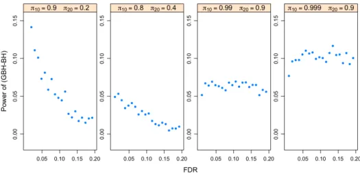
For the oracle case with independent p-values, Figure 3indicates that the GBH pro-cedure outperforms the BH propro-cedure in all four cases, especially when πg,0’s are close to 1 (the last two panels). The more the groups differ in πg,0, the larger the difference is obtained in the power of the two procedures. This is also true forp-values with the PRDS property. Figure 4 shows the power difference between the GBH and BH procedures for

p-values under model (4.1) with ξ1 =ξ2 = 0.5. All points being above zero indicates the GBH procedure outperforms the BH procedure for all four cases.

For the adaptive case with independent p-values, we estimate the unknown πg,0’s using either the TST or LSL method introduced in section 2.3. Figure 5 indicates that the average of the false discovery proportion (FDP) is controlled at pre-specified FDR level for both the BH and GBH procedures with either the TST or LSL method. The power improvement of the adaptive GBH over the adaptive BH procedure is shown in Figure6. Both the TST GBH and the LSL GBH procedures are more powerful than the corresponding adaptive BH procedures.

We also analyze the performance of the adaptive GBH procedure for weighting scheme other than πg,0/πg,1. According to (2.6), when Ug is uniform, the Bayesian FDR is [πg,0/Dg(p)]p, whereDg(p) is the distribution function of p-values in group g. It’s there-fore natural to consider the weight ˆπg,0/D˜g(p), where ˜Dg is the empirical distribution, as pointed out by a referee. Although this weight takes into consideration of the distribu-tion of p-values in each group, the power of the adaptive procedure using this weight is often low in the situation where we have sparse signals and estimating the alternative distribution is difficult.

5

APPLICATIONS

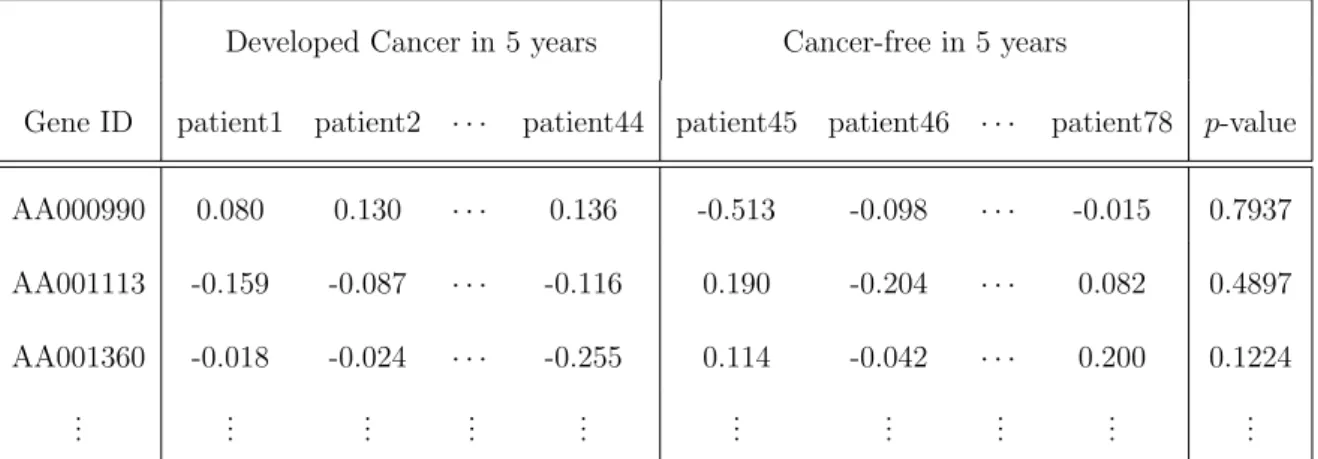
Van’t Veer et al. (2002) used microarrays to study the primary breast tumors of 78 young patients, of which 44 developed cancer in less than 5 years and the other 34 were cancer free during that period. In total 24,184 genes were monitored andp-values were obtained for each gene by comparing the mean ratio of log₁₀ intensities. A fraction of the data is listed in Table 1.

In order to apply the GBH procedure which makes use of the group structure, we need to stratify the genes first. Here we consider two grouping strategies.

5.1

Grouping using Gene Ontology (GO)

The GO project (The Gene Ontology Consortium 2000) provides detailed annotations for a gene product’s biology. It consists of three ontologies, namely Biological Process, Molecular Function and Cellular Component, each representing a key concept in Molecu-lar Biology. The GO terms are classified into one of the three ontologies. Based on the GO terms, one can construct a top-down tree diagram, in which the higher nodes represent more general biological concepts.

The tree structure provides the idea of GO grouping which can be summarized as follows. After choosing one of the three ontologies, say Biological Process, some higher nodes are selected as ancestors according to the generic GO slim file, which contains the broad overview of each ontology without the detail of each GO terms (accessible at

http://www.geneontology.org/GO.slims.shtml). Next, for those genes with GO IDs,

we trace them upward to the nodes we have chosen. Genes that share common ancestors are then grouped together. The biggest concern for GO grouping in our case is that the mapping rate is low. Even though the GO consortium updates their data base on a daily basis, not every gene in our data has a GO ID. For our case, 9,492 of the 24,184 genes have the annotation information for Biological Process, therefore the mapping rate for our data is 9492/24184≈39%.

However, we may still use the remaining 9,492 genes to see the difference of using group information in multiple hypothesis testings. We first divide the genes into four groups with respect to Biological Process, i.e., 1) Cell communication; 2) Cell growth

and-or maintenance; 3) Development; and 4) Multi-function. The results for the adaptive BH and GBH procedures are listed in Table 2. For simplicity, we just report the results for the LSL method.

At FDR level 0.15, Table 2 indicates that the adaptive GBH procedure focuses more on groups with smaller estimated πg,0’s, i.e., groups 2) and 4), and is able to discover genes that are not detectable using the adaptive BH procedure. In fact, as shown in Figure2, using either the LSL or TST method, the adaptive BH procedure cannot detect any signals when the FDR level is less than 0.15.

Even though the mapping rate for this data set is low, the idea of GO grouping could be a good choice if the data were collected in terms of GO identities; or the mapping between the GO ID and other gene IDs (e.g., GenBank Accession Number) was more complete. Then each group may correspond to different biological processes or genetic functions within the tumor and the GBH method can help us to find more signals among desired groups.

5.2

Grouping using

k

-means clustering

Another grouping idea is to apply clustering. Here we choose k-means clustering with initial points satisfying maximum separation rule based on all the 78 samples. Note that we are not just clustering the p-values. Unlike GO grouping, k-means clustering makes use of the whole data set and we do not have to worry about the mapping rate. Although we do have the difficulties regarding cluster analysis, e.g., the choice of initial points, number of clusters, and the interpretation of each cluster, we use it as an illustrative example to compare the performances of the adaptive BH and GBH procedures.

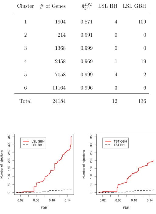
within each cluster there are at least 200 genes. Table 3 shows the results for the two procedures using the LSL method at FDR level 0.1. Most of the additional discoveries found by the adaptive GBH procedure come from the first cluster, which is expected to contain more signals because the estimated πg,0 is relatively smaller than the others. Gene-annotation enrichment analysis confirms that those 109 genes selected by the GBH procedure in the first cluster are closely associated with cell cycle, mitosis, chromosome segregation and phosphoprotein, which are common factors related to breast cancer. Similar analyses on the four and five-cluster cases indicate that the number of genes detected by the adaptive GBH procedure is 145 and 226, respectively. Out of those genes, 94 of them are overlapping with the six-cluster case. Comparing with an average of eight genes discovered by random grouping, which assigns groups randomly with the same group sizes as the above three cases, clustering and using the GBH procedure is advantageous in our case.

For comparison of the two procedures over a range of FDR levels, Figure 1shows the increment in the number of signals detected by the adaptive GBH over BH procedure for both the LSL and TST methods. This indeed shows that by applying the GBH procedure, more signals can be detected.

6

SUMMARY

We have presented a new approach of p-value weighting procedure GBH for controlling the FDR when the hypotheses are believed to have some group structure. We prove that it controls the FDR for hypotheses with the positive regression dependence property when the proportions of true null hypotheses πg,0’s are known in each group. The weighting scheme (πg,0/πg,1) for thep-values in each group makes it possible to focus on groups that

are expected to have more signals.

By estimating πg,0 for each group, we propose the adaptive GBH procedure and show that it controls the FDR asymptotically under weak dependence. We demonstrate the benefit of the adaptive GBH over BH by two methods of estimating πg,0, namely the LSL (Benjamini and Hochberg 2000) and the TST (Benjamini et al. 2006) estimators. As we have pointed out, the choice of the estimator for πg,0 in general does not affect the performance of the adaptive GBH procedure. In practice, people may choose the estimator based on their own preference.

7

APPENDIX: PROOFS

Proof of Theorem 1. The proof is based on the proof of Theorem 4.1 in Finner, Dick-haus and Roters (2009). Let ϕ= (ϕ1, . . . , ϕN) be the multiple testing procedure.ϕi = 0 means retaining Hi and ϕi = 1 means rejecting Hi. The FDR for oracle GBH is

FDR(ϕGBH) = E

"

V R∨1

#

=E

"

V R∨1

X

j∈IN

{R=j}

# = K X g=1 X

i∈Ig,0

X

j∈IN

1 j Pr

R=j, ϕg,i = 1

= K X g=1 X

i∈Ig,0

X

j∈IN

1 j Pr

R=j,πg,0 πg,1

Pg,i ≤ j Nα

w .

Note that if πg,0 = 0 or πg,0 = 1 for some g, that group doesn’t contribute to the FDR because Ig,0 = ∅ if πg,0 = 0 and Pr(R = j,π_πg,_g,0₁Pg,i ≤ _Njαw) = 0 if πg,0 = 1 (we treat

πg,0/πg,1 as∞). Let η ={g :πg,0 ∈(0,1)}. Then

FDR(ϕGBH) =

X

g∈η

X

i∈Ig,0

X

j∈IN

1 j Pr

R=j,πg,0 πg,1

Pg,i ≤ j Nα

Using the proof of Theorem 4.1 in Finner, Dickhaus and Rosters (2009), we have

FDR(ϕGBH) ≤

X

g∈η

πg,1αw

πg,0N

X

i∈Ig,0

Pr(R≥1|P_g,iw ≤ 1

Nα w₎

= X

g∈η

πg,1αw

πg,0N

X

i∈Ig,0

1 = X

g∈η

πg,1αw

πg,0N

·ngπg,0

=

P

g∈ηngπg,1

PK

g=1ngπg,1

α ≤α.

Proof of Lemma 1. For the unweighted case, the expected number of rejections of BH procedure for a given threshold t, where t≤˜t= (1−π0) max

g πg,0/πg,1 is

E

h

RBH(t)

i = _E K X g=1 X

j∈Ig

{π0Pj ≤t}

= _E

K

X

g=1

X

j∈Ig,0 {Pj ≤

t π0

}+ X

j∈Ig,1 {Pj ≤

t π0

}

≤ N t+

K

X

g=1

ngπg,1F

t

π0

.

Similarly, the expected number of rejections of GBH procedure fort ≤˜_{t is}

E

h

RGBH(t)

i = _E K X g=1 X

j∈Ig

{πg,0

πg,1

(1−π0)Pj ≤t}

= N t+ K

X

g=1

ngπg,1F

π_g,1t

πg,0(1−π0)

Let g = ngπg,1/P_gngπg,1 and xg = πg,0(1−π0)/πg,1. Now that x 7→ F(t/x) is convex for all x≥˜t. We have F(t/P

ggxg)≤

P

ggF(t/xg), i.e., F t

π0

≤ _P 1

gngπg,1 K

X

g=1

ngπg,1F

π_g,1t

πg,0(1−π0)

.

Therefore,_EhRBH(t)

i

≤_EhRGBH(t)

i

for t≤˜_t.

any t≥0,

sup t

|De_g(t)−D_g(t)| ≤ sup

t

ng,0

ng 1 ng,0

X

i∈Ig,0

{Pi ≤t} −πg,0Ug(t)

+ sup t

ng,1

ng 1 ng,1

X

i∈Ig,1

{Pi ≤t} −πg,1Fg(t)

≤

ng,0

ng

−πg,0

+πg,0sup

t

1 ng,0

X

i∈Ig,0

{Pi ≤t} −Ug(t)

+

ng,1

ng

−πg,1

+πg,1sup

t

1 ng,1

X

i∈Ig,1

{Pi ≤t} −Fg(t)

where sup_t|n−_g,1₀P

i∈Ig,0{Pi ≤t} −Ug(t)|

a.s.

→ 0 and sup_t|{n−_g,1₁P

i∈Ig,1{Pi ≤t} −Fg(t)|

a.s.

→ 0

by Glivenko-Cantelli Theorem. Therefore, sup_t|De_g(t)−D_g(t)|

a.s.

→ 0.

Proof of Theorem 2. Theorem 4 generalizes this theorem. See the proof of Theorem 4.

Proof of Theorem 3. Under the conditions thatUg(t) =U(t) =t andFg(t) =F(t) for all g, in the proof of Lemma 2, we show that G(a, t)≥ C(t/π0) for all 0 ≤t ≤ mingag. Since G(a, π0) ≤ π0 = t/C(t/π0)|t=π0 and both G(a, t) and t/C(t/π0) are increasing,

we have G(a, t) ≥ C(t/π0) for all 0 ≤ t ≤ maxgag. Deduce B(a, t) ≤ t/C(t/π0) for

t ∈ c(a). Therefore t∗_BH ≤ t∗_GBH. Conditions limt↓0t/C(t/π) ≤ α and π0 ≥ α guarantee that t∗_BH >0.

Note that both G(a, t) and t/C(t/π0) are continuous, we have

t∗_BH C(t∗_BH/π0)

= t

∗ GBH G(a, t∗_GBH).

Sincet∗_BH ≤t∗_GBH, deduce C(t∗_BH/π0)≤G(a, t∗GBH). For the adaptive BH procedure, the number of rejections RBH( ˆTBH) =

P

i∈IN{Pi ≤

ˆ

TBH/πˆ0}=N ·CN( ˆTBH/πˆ0), and

|CN( ˆTBH/πˆ0)−C(t∗BH/π0)| ≤ sup t≥0

|CN(t/ˆπ0)−C(t/πˆ0)| +|C( ˆTBH/πˆ0)−C(t∗BH/π0)|,

where sup_t≥0|CN(t/πˆ0)−C(t/πˆ0)| a.s.

→ 0 by Glivenko-Cantelli theorem and|C( ˆTBH/πˆ0)−

C(t∗_BH/π0)| P

→0 by continuous mapping theorem. ThereforeCN( ˆTBH/πˆ0) P

→C(t∗_BH/π0). Analogously one can show that GN(ˆa,TˆGBH)

P

→ G(a, t∗_GBH). A more generalized ar-gument is shown in the proof of Theorem 4. By dominant convergence theorem we have N−1_E[RBH( ˆTBH)] → C(t∗BH/π0) and N−1E[RGBH( ˆTGBH)] → G(a, t∗GBH). There-fore _E[RBH( ˆTBH)]/E[RGBH( ˆTGBH)]≤1 +o(1).

Proof of Theorem 4. The proof applies Glivenko-Cantelli theorem as in Storey et al. (2004) and Genovese et al. (2006). LetS =c(ˆa)∪c(ρ). For any t ∈S, we have

sup t∈S

|GN(ˆa, t)−G(ρ, t)| ≤sup t≥0

|GN(ˆa, t)−G(ˆa, t)|+ sup t≥0

|G(ˆa, t)−G(ρ, t)|.

Note that for t ≥0,

sup t

|GN(ˆa, t)−G(ˆa, t)| = 1 N

K

X

g=1

ngsup t

|Deg(t/ˆag)−Dg(t/ˆag)|

≤ 1

N K

X

g=1

ngsup t

|De_g(t)−D_g(t)|

a.s.

→ 0, (7.1)

where the last step is implied by Lemma 2. On the other hand,

sup t≥0

|G(ˆa, t)−G(ρ, t)|= 1 N

K

X

g=1

ngsup t≥0

|Dg(t/ˆag)−Dg(t/ρg)|.

Since Dg is continuous on [0,+∞) and limt→∞Dg(t) = 1 is finite, Dg is uniform contin-uous. By continuous mapping theorem, |t/ˆag−t/ρg|

P

→ 0. Therefore sup_t∈S|Dg(t/aˆg)− Dg(t/ρg)|

P

→0. So we have sup_t∈S|GN(ˆa, t)−G(ρ, t)| P

→0. LetBN(ˆa, t) =

P

gng,0t/aˆg

N·GN(ˆa,t) . According to (2.16) and (3.6), ˆTGBH = supt∈c(ˆa){t:BN(ˆa, t)≤

α} and t∗_GBH = sup_t∈c(ρ){t : B(ρ, t) ≤ α}, where B(ρ, t) = P

gπgπg,0t/ρg

G(ρ,t) . Note that the assumption limt↓0B(ρ, t)6=α implies t∗GBH >0.

We first show ˆTGBH P

→ t∗_GBH. For any ξ > 0, note that B(ρ, t) is increasing for t≥maxgρg, therefore B(ρ, t∗GBH +ξ)> α, otherwise it contradicts with t

∗

supremum. Fix δ >0, for anyδ0 ≥δ, let t0 =t∗_GBH +δ0. Then

inf

δ0_≥δBN(ˆa, t

0

) = inf

δ0_≥δ

1 N

P

gng,0t0/ˆag GN(ˆa, t0)

≥ inf

δ0_≥δ P

gπgπg,0t0/ρg−

P

g|ng,0/Nˆag−πgπg,0/ρg|t0 G(ρ, t0_{) + sup}

t∈S|GN(a, tˆ )−G(ρ, t)|

≥ 1−1

[1/infδ0_≥δB(ρ, t0)] +₂

,

where1 =P_g|ng,0/Nˆag−πgπg,0/ρg|/(P_gπgπg,0/ρg), and2 = supt∈S|GN(ˆa, t)−G(ρ, t)|/(P_gπgπg,0t0/ρg). Since 1, 2

P

→ 0 and infδ0_≥δB(ρ, t0) > α, it can be derived that Pr(T

δ0_≥δ{B_N(ˆa, t0) >

α})→1 which implies Pr( ˆTGBH < t∗GBH +δ)→1.

On the other hand, sinceB(ρ, t) has a non-zero derivative att∗_GBH, it must be positive, otherwiset∗_GBH cannot be the supremum of alltsuch thatB(ρ, t)≤α. Thus, t7→B(ρ, t) is an increasing function and for any ξ > 0, B(ρ, t∗_GBH −ξ) < α. For any δ > 0, let t◦ =t∗_GBH −δ,

BN(ˆa, t◦) = 1 N

P

gng,0t◦/ˆag GN(ˆa, t◦)

≤

P

gπgπg,0t◦/ρg+

P

g|ng,0/Nˆag−πgπg,0/ρg|t◦ G(ρ, t◦_)−sup

t∈S|GN(a, tˆ )−G(ρ, t)|

≤ 1 +1

[1/B(ρ, t◦_)]− 2

,

where 1, 2 P

→ 0 and B(ρ, t◦) < α. Then Pr(BN(ˆa, t◦) < α) → 1. Deduce Pr( ˆTGBH > t∗_GBH −δ)→1. Combine this and previous result we get ˆTGBH

P

→t∗_GBH. Next, we prove F DR( ˆTGBH)≤α/ming{bg}+o(1). Let

HN(ˆa, t) = 1 N K X g=1 X

i∈Ig,0

{Pi ≤t/aˆg}

be the empirical distribution of p-values under null hypothesis for adaptive GBH pro-cedure. Note that ˆTGBH

P

→ t∗_GBH implies Pr( ˆTGBH > t∗GBH − δ) → 1 for any δ > 0. Since t∗_GBH > 0, deduce Pr( ˆTGBH > 0) → 1. On the other hand, the assumption ¯ζ < 1 rules out the situation where ˆTGBH/ˆag →0 for all groups. Therefore Pr(P_gP_i∈Ig{Pi ≤

ˆ

TGBH/ˆag} ≥1)→1. Then the false discovery proportion (FDP) is

F DP( ˆTGBH) =

N−1PK

g=1

P

i∈Ig0{Pi ≤

ˆ

TGBH/ˆag} N−1PK

g=1

P

i∈Ig{Pi ≤

ˆ

TGBH/ˆag}

= HN(ˆa, ˆ TGBH) GN(ˆa,TˆGBH) ,

where HN(ˆa,TˆGBH) satisfies

HN(ˆa,

ˆ

TGBH)− 1 N

K

X

g=1

ng,0Ug( ˆTGBH/ˆag)

≤ 1 N K X g=1

ng,0 sup t∈c(ˆa)

1 ng,0

X

i∈Ig,0

{Pi ≤t/ˆag} −Ug(t/aˆg)

≤ 1 N K X g=1

ng,0sup t≥0

1 ng,0

X

i∈Ig,0

{Pi ≤t} −Ug(t)

.

By condition (3.2), Glivenko-Cantelli Theorem implies sup_t≥0| 1 ng,0

P

i∈Ig,0{Pi ≤ t} −

Ug(t)| a.s.

→ 0. Therefore,

HN(ˆa,

ˆ

TGBH)− 1 N

K

X

g=1

ng,0Ug( ˆTGBH/aˆg)

a.s.

→0. (7.2)

Now that ˆTGBH P

→t∗_GBH and by (3.1), 1

N K

X

g=1

ng,0Ug( ˆTGBH/aˆg) P

−→

K

X

g=1

πgπg,0Ug(t∗GBH/ρg). (7.3)

Combine (7.2) and (7.3) we have

HN(ˆa,TˆGBH) P

→

K

X

g=1

πgπg,0Ug(t∗GBH/ρg). (7.4)

On the other hand,

|GN(ˆa,TˆGBH)−G(ρ, t∗GBH)| ≤ |GN(ˆa,TˆGBH)−G(ˆa,TˆGBH)| +|G(ˆa,TˆGBH)−G(ρ, t∗GBH)|

≤ sup

t≥0

|GN(ˆa, t)−G(ˆa, t)|+|G(ˆa,TˆGBH)−G(ρ, t∗GBH)|

where sup_t≥0|GN(ˆa, t)−G(ˆa, t)| a.s.

→ 0 by (7.1) and |G(ˆa,TˆGBH)−G(ρ, t∗GBH)| P

→ 0 by

continuous mapping theorem. Therefore,

GN(ˆa,TˆGBH) P

Since t∗_GBH >0 and ¯ζ <1, we have G(ρ, t∗_GBH)>0. By (7.4) and (7.5),

F DP( ˆTGBH) P

→

PK

g=1πgπg,0Ug(t ∗

GBH/ρg) G(ρ, t∗_GBH) . By dominated convergence theorem,

F DR( ˆTGBH) =E

h

F DP( ˆTGBH)

i

→

PK

g=1πgπg,0Ug(t∗GBH/ρg)

G(ρ, t∗_GBH) . (7.6) Note that ζg ≥ bgπg,0 for some bg > 0. Deduce ρg ≥ bgπg,0/(1−ζg). Since Ug(t) ≤ t for allt ≥0, we have

PK

g=1πgπg,0U(t ∗

GBH/ρg) G(ρ, t∗

GBH)

≤ 1

ming{bg}

(1−ζ¯)t∗_GBH G(ρ, t∗

GBH)

≤ α

ming{bg} .

Hence, F DR( ˆTGBH)≤α/ming{bg}+o(1).

References

[1] Benjamini, Y., and Hochberg, Y. (1995), “Controlling the False Discovery Rate: A Practical and Powerful Approach to Multiple Testing,”Journal of the Royal Statis-tical Society, Ser. B, 57, 289-300.

[2] —— (1997), “Multiple Hypothesis Testing with Weights,” Scandinavian Journal of Statistics, 24, 407-418.

[3] —— (2000), “On the Adaptive Control of the False Discovery Rate in Multiple Test-ing with Independent Statistics,” Journal of Educational and Behavioral Statistics, 25, 60-83.

[4] Benjamini, Y., and Yekutieli, D. (2001), “The Control of the False Discovery Rate in Multiple Testing under Dependency,” The Annals of Statistics, 29, 1165-1188.

[5] Benjamini, Y., Krieger, M. A., and Yekutieli, D. (2006), “Adaptive Linear Step-up Procedures That Control the False Discovery Rate,” Biometrika, 93, 3, 491-507.

[6] Dmitrienko, A., Offen, W. W., and Westfall, H. P. (2003), “Gatekeeping Strategies for Clinical Trials that Do Not Require All Primary Effects to be Significant,”Statistics In Medicine, 22, 2387-2400.

[7] Efron, B. (2008), “Simultaneous Inference: When Should Hypothesis Testing Prob-lems be Combined?” The Annals of Applied Statistics, 2, 1, 197-223.

[8] Efron, B., and Tibshirani, R. (2002), “Empirical Bayes Methods and False Discovery Rates for Microarrays,” Genetic Epidemiology, 23, 70-86.

[9] Efron, B., Tibshirani, R., Storey, J. D., and Tusher, V. (2001), “Empirical Bayes Analysis of a Microarray Experiment,” Journal of the American Statistical Associa-tion, 96, 1151-1160.

[10] Finner, H., Dickhaus, T., and Roters, M. (2007), “Dependency and False Discovery Rate: Asymptotics,”The Annals of Statistics, 35, 1432-1455.

[11] ——(2009), “On the False Discovery Rate and an Asymptotically Optimal Rejection Curve,”The Annals of Statistics, 37, 2, 596-618.

[12] Finner, H. and Roters, M. (2001), “On the False Discovery Rate and Expected Type 1 Errors,” Biometrical Journal, 43, 8, 985-1005.

[13] Genovese, C. R., Roeder, K., and Wasserman, L. (2006), “False Discovery Control with P-Value Weighting,” Biometrika, 93, 509-524.

[14] Genovese, C. R., and Wasserman, L. (2004), “A Stochastic Process Approach to False Discovery Control,” The Annals of Statistics, 32, 1035-1061.

[15] Hsueh, H., Chen, J., and Kodell, R. (2003), “Comparison of Methods for Estimating the Number of True Null Hypotheses in Multiplicity Testing,” Journal of Biophar-maceutical Statistics, 13, 4, 675-689.

[16] Holm, S. (1979), “A Simple Sequentially Rejective Multiple Test Procedure,” Scan-dinavian Journal of Statistics, 6, 65-70.

[17] Jin, J., and Cai, T. (2007), “Estimating the Null and the Proportion of Non-null Effects in Large-scale Multiple Comparisons,” Journal of the American Statistical Association, 102, 495-506.

[18] Meinshausen, N., and Rice, J. (2006), “Estimating the Proportion of False Null Hy-potheses among a Large Number of Independently Tested HyHy-potheses,” The Annals of Statistics, 34, 1, 373-393.

[19] Quackenbush, J. (2001), “Computational Analysis of Microarray Data,” Nature Re-view Genetics, 2, 418-427.

[20] Roeder, K., Bacanu, SA., Wasserman, L., and Devlin, B. (2006), “Using Linkage Genome Scans to Improve Power of Association in Genome Scans,” The American Journal of Human Genetics, 78, 2, 243-252.

[21] Rubin, D., van der Laan, M., and Dudiot, S. (2005), “Multiple Testing Procedures Which Are Optimal at a Simple Alternative,” Technical report 171, University of California, Berkeley, Division of Biostatistics.

[22] Schweder, T., and Spjøtvoll, E. (1982), “Plots of P-values to Evaluate Many Tests Simultaneously,” Biometrika, 69, 493-502.

[23] Storey, J. D. (2002), “A Direct Approach to False Discovery Rates,” Journal of the Royal Statistical Society, Ser. B, 64, 479-498.

[24] Storey, J. D., Taylor, J. E., and Siegmund, D. (2004), “Strong Control, Conservative Point Estimation, and Simultaneous Conservative Consistency of False Discovery Rates: A Unified Approach,” Journal of the Royal Statistical Society, Ser. B, 66, 187-205.

[25] Sun, L., Craiu, R. V., Paterson, A. D., and Bull, S. B. (2006), “Stratified False Discovery Control for Large-Scale Hypothesis Testing with Application to Genome-Wide Association Studies,”Genetic Epidemiology, 30, 6, 519-530.

[26] The Gene Ontology Consortium. (2000), “Gene Ontology: Tool for the Unification of Biology,” Nature Genetics, 25, 25-29.

[27] van’t Veer, L. J. et al. (2002), “Gene Expression Profiling Predicts Clinical Outcome of Breast Cancer,” Nature, 415, 530-536.

[28] Wasserman, L., and Roeder, K. (2006), “Weighted Hypothesis Testing,” Technical report, Carnegie Mellon University, Department of Statistics.

Table 1: Part of the breast cancer data set in van’t Veer (2002).

Developed Cancer in 5 years Cancer-free in 5 years

Gene ID patient1 patient2 · · · patient44 patient45 patient46 · · · patient78 p-value AA000990 0.080 0.130 · · · 0.136 -0.513 -0.098 · · · -0.015 0.7937 AA001113 -0.159 -0.087 · · · -0.116 0.190 -0.204 · · · 0.082 0.4897 AA001360 -0.018 -0.024 · · · -0.255 0.114 -0.042 · · · 0.200 0.1224

..

. ... ... ... ... ... ... ... ... ... Note: The entries are adjusted log₁₀(red/green) ratios from cDNA microarrays. Thep-values were

calculated based on a two-samplet-test for each gene.

Table 2: Comparison of the adaptive LSL GBH and the adaptive LSL BH procedures for GO grouping. FDR level = 0.15.

Group # of Genes πˆLSL

g,0 LSL BH LSL GBH

1) Cell communication 593 0.995 0 3

2) Cell growth/maintenance 4142 0.987 0 13

3) Development 434 0.989 0 0

4) Multi-function 4323 0.983 0 25

Table 3: Comparison of the adaptive LSL GBH and the adaptive LSL BH procedures for

k-means grouping. FDR level = 0.1.

Cluster # of Genes πˆ_g,LSL₀ LSL BH LSL GBH

1 1904 0.871 4 109

2 214 0.991 0 0

3 1368 0.999 0 0

4 2458 0.969 1 19

5 7058 0.999 4 2

6 11164 0.996 3 6

Total 24184 12 136

Figure 1:Breast cancer study, 24,184 genes. Plot shows the number of signals detected by GBH and BH procedures versus pre-specified FDR level. Left panel: adaptive LSL GBH procedure. Right panel: adaptive TST GBH procedure. Details for LSL and TST approaches are in section 2.3. Genes are assigned into six groups using k-means clustering. Data from van’t Veer et al (2002).

Figure 2: Breast cancer study, 9,492 genes. The plots show the number of genes detected by the adaptive BH and GBH procedures using Gene Ontology grouping. Left panel: the LSL method. Right panel: the TST method. Data from van’t Veer et al (2002).

Figure 3: Power curves of the oracle BH and GBH procedures for independent p-values. The

p-values are generated based on model (4.1) with ξ1 =ξ2 = 0 and n= 10,000 for each group. Each panel corresponds to one combination ofπg,0’s for two groups.

Figure 4: Power differences of the oracle BH and GBH procedures forp-values with the PRDS property. Thep-values are generated based on model (4.1) with ξ1 =ξ2 = 0.5 and n= 10,000

for each group. Each panel corresponds to one combination of πg,0’s for two groups.

Figure 5: Comparison of the average FDP and the pre-specified FDR for the adaptive BH and GBH procedures. The dash line is the 45-degree line. The p-values are generated based on model (4.1) with ξ1 = ξ2 = 0 and n = 10,000 for each group. Each point of the FDP is the

Figure 6:Power curves of the adaptive BH and GBH procedures for independentp-values. The

p-values are generated based on model (4.1) with ξ1 =ξ2 = 0 and n= 10,000 for each group. Each panel corresponds to one combination ofπg,0’s for two groups.