Figure 2.1: Center of mass of four points.

Chapter 2

B´

EZIER CURVES

B´ezier curves are named after their inventor, Dr. Pierre B´ezier. B´ezier was an engineer with the Renault car company and set out in the early 1960’s to develop a curve formulation which would lend itself to shape design.

Engineers may find it most understandable to think of B´ezier curves in terms of the center of mass of a set of point masses. For example, consider the four massesm0,m1,m2, andm3 located at pointsP0,P1,P2,P3. The center of mass of these four point masses is given by the equation

P0

P₁ P₂

P3 P

Figure 2.1: Center of mass of four points.

P = m0P0 + m1P1 + m2P2 + m3P3

m0 + m1 + m2 + m3

.

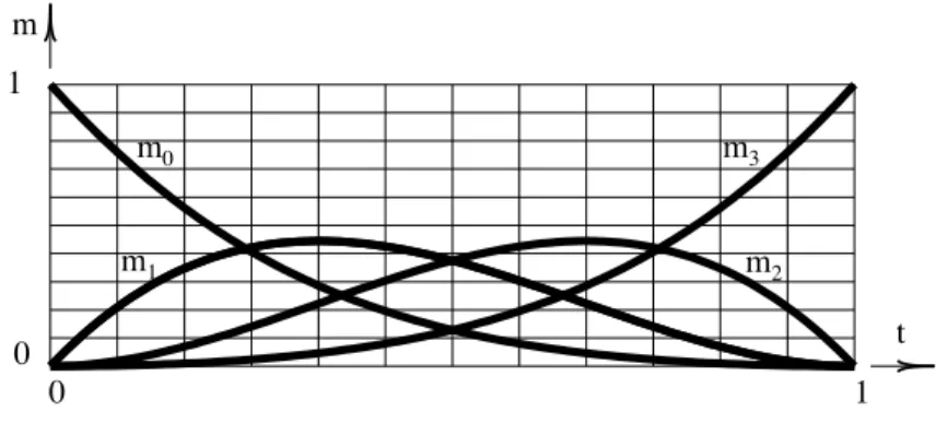
Next, imagine that instead of being fixed, constant values, each mass varies as a function of some parametert. In specific, let m0 = (1−t)3, m1 = 3t(1−t)2, m2 = 3t2(1−t) and m3 = t3. The values of these masses as a function oft is shown in this graph: Now, for each value of t, the

masses assume different weights and their center of mass changes continuously. In fact, as tvaries

between 0 and 1, a curve is swept out by the center of masses. This curve is a cubic B´ezier curve – cubic because the mass equations are cubic polynomials in t. Notice that, for any value of t, m0 + m1 + m2 + m3 ≡ 1, and so we can simply write the equation of this B´ezier curve as

P = m0P0 + m1P1 + m2P2 + m3P3.

Note that whent= 0,m0 = 1 andm1=m2=m3= 0. This forces the curve to pass through

P0. Also, whent= 1,m3= 1 andm0=m1=m2= 0, thus the curve also passes through pointP3. Furthermore, the curve is tangent toP0−P1 and P3−P2. These properties make B´ezier curves

m 1

0

0 1

t m0

m₁ m₂

m3

Figure 2.2: Cubic B´ezier blending functions.

P0

P₁ P₂

P3

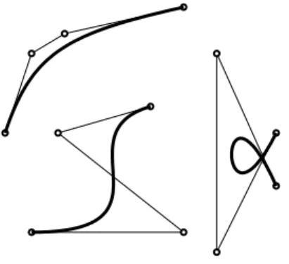
15 an intuitively meaningful means for describing free-form shapes. Here are some other examples of cubic B´ezier curves which illustrate these properties. These variable massesmi are normally called

Figure 2.4: Examples of cubic B´ezier curves.

blending functionsand their locationsPi are known ascontrol points or B´ezier points. If we draw

straight lines between adjacent control points, as in a dot to dot puzzle, the resulting figure is known as a control polygon. The blending functions, in the case of B´ezier curves, are known asBernstein polynomials. We will later look at other curves formed with different blending functions.

B´ezier curves of any degree can be defined. Figure 2.5 shows sample curves of degree one through four. A degreenB´ezier curve hasn+ 1 control points whose blending functions are denotedBn

i(t),

Degree 1 Degree 2

Degree 3 Degree 4

Figure 2.5: B´ezier curves of various degree. where

Bin(t) =

!_n

i

"

(1₋t)n−iti, i= 0,1, ..., n.

Recall that#n i

$_{is called abinomial coefficient, sometimes spoken “}

n- choose- i”, and is equal to

n!

i!(n−i)!. In our introductory example, n = 3 and m0 = B 3

0 = (1−t)3, m1 = B13 = 3t(1−t)2,

of degreen. The equation of a B´ezier curve is thus:

P(t) =

n

%

i=0 !_n

i

"

(1₋t)n−iti_P

i. (2.1)

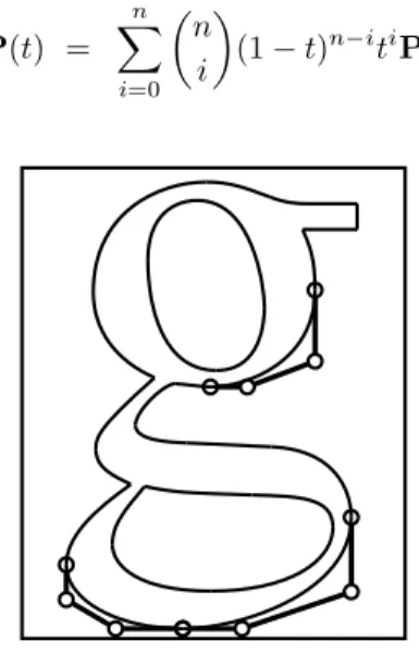
Figure 2.6: Font definition using B´ezier curves.

A common use for B´ezier curves is in font definition. Figure 2.6 shows the outline a letter “g” created using B´ezier curves. All PostScript font outlines are defined use cubic and linear B´ezier curves.

2.1

B´

ezier Curves over Arbitrary Parameter Intervals

Equation 2.1 gives the equation of a B´ezier curve which starts at t = 0 and ends at t = 1. It is

useful, especially when fitting together a string of B´ezier curves, to allow an arbitrary parameter interval:

t0≤t≤t1

such thatP(t0) =P0 andP(t1) =Pn. This can be accomplished by modifying equation 2.1:

P(t) =

&n i=0

#n i

$₍

t1−t)n−i(t−t0)iPi

(t1−t0)n

= (2.2)

n

%

i=0 !_n

i

" (t1−t

t1−t0

)n−i₍t−t0

t1−t0 )i_Pi.

2.2

Subdivision of B´

ezier Curves

The most fundamental algorithm for dealing with B´ezier curves is the subdivision algorithm. This was devised in 1959 by Paul de Casteljau (who was working for the Citroen automobile company) and is referred to as thede Casteljau algorithm. It is sometimes known as thegeometric construction algorithm.

Consider a B´ezier curve defined over the parameter interval [0,1]. It is possible to subdivide

2.2. SUBDIVISION OF B ´EZIER CURVES 17 τ _≤t_≤1. These two new B´ezier curves, considered together, are equivalent to the single original

curve from which they were derived.

As illustrated in Figure 2.7, begin by adding a superscript of 0 to the original control points, then compute

Pj

i = (1−τ)Pj−

1

i +τPj−

1

i+1; j= 1, . . . , n; i= 0, . . . , n−j. (2.3) Then, the curve over the parameter domain 0_≤t_≤τis defined using control pointsP0

0,P10,P20, . . . ,Pn0 and the curve over the parameter domainτ_≤t_≤1 is defined using control pointsPn

0,Pn1−1,P2n−2, . . . ,P0n.

P₀0 P₁0

P₂0

P₃0 P₀1

P₁1

P₂1 P₀2

P₁2 P₀3

t = .4

P₀0 P₁0

P₂0

P₃0 P₀1

P₁1

P₂1

P₀2 _P

12

P₀3

t = .6

Figure 2.7: Subdividing a cubic B´ezier curve.

Figure 2.8 shows that when a B´ezier curve is repeatedly subdivided, the collection of control polygons converge to the curve.

1 curve 2 curves

4 curves 8 curves

Figure 2.8: Recursively subdividing a quadratic B´ezier curve.

One immediate value of the de Casteljau algorithm is that it provides a numerically stable means of computing the coordinates of any point along the curve. Its extension to curves of any degree should be obvious.

It can be shown that if a curve is repeatedly subdivided, the resulting collection of control points converges to the curve. Thus, one way of plotting a B´ezier curve is to simply subdivide it an appropriate number of times and plot the control polygons.

The de Casteljau algorithm works even for parameter values outside of the original parameter interval. Fig. 2.9 shows a quadratic B´ezier curve “subdivided” atτ= 2. The de Castelau algorithm

P₀0 P₁0

P₂0 P₀1

P₁1

P₀2

t = 2

Figure 2.9: Subdividing a quadratic B´ezier curve.

is numerically stable as long as the parameter subdivision parameter is within the parameter domain of the curve.

2.3

Degree Elevation

Another useful algorithm is the degree elevation algorithm. This has many uses. For example, some modeling systems use only cubic B´ezier curves. However, it is important to be able to represent degree two curves exactly. A curve of degree two can be exactly represented as a B´ezier curve of degree three or higher. In fact, any B´ezier curve can be represented as a B´ezier curve of higher degree.

We illustrate by raising the degree of a cubic B´ezier curve to degree four. We denote the cubic B´ezier curve in the usual way:

x(t) = P0B03(t) + P1B13(t) + P2B23(t) + P3B33(t)

Note that this curve is not changed at all if we multiply it by [t + (1 ₋ t)] _≡ 1. However,

multiplication in this way does serve to raise the degree of the B´ezier curve by one. Its effect in the cubic case is to create five control points from the original four. Those five control points thus define a degree four B´ezier curve which is precisely the same as the original degree three curve. The new control pointsP∗

i are easily found as follows:

P∗

0 = P0

P∗

1 =

1 4P0 +

3 4P1

2.3. DEGREE ELEVATION 19

P₀* _P 0 1/4

1/2 P₁*

P₁ old P₂* _P

2

P₃*

P₄* P₃ new

Figure 2.10: Degree elevation.

P∗

2 =

2 4P1 +

2 4P2

P∗

3 =

3 4P2 +

1 4P3

P∗

4 = P3 This works for any degreenas follows:

P∗

i = αiPi−1 + (1−αi)Pi, αi = i

n+ 1.

Furthermore, this degree elevation can be applied repeatedly to raise the degree to any level, as shown in Figure 2.11. Note that the control polygon converges to the curve itself.

Degree 2 Degree 3 Degree 4

Degree 5 Degree 6 Degree 7

2.4

Distance between Two B´

ezier Curves

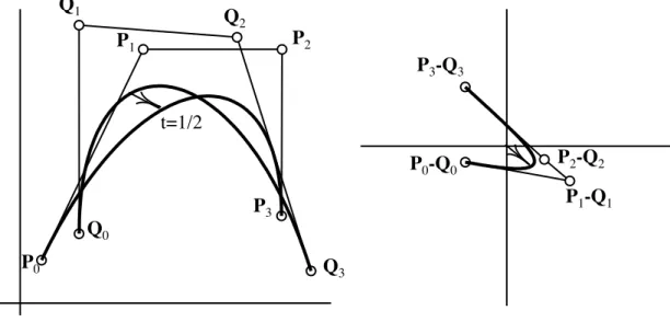
The problem often arises of determining how closely a given B´ezier curve is approximated by a second B´ezier curve. For example, if a given cubic curve can be adequately represented by a degree elevated quadratic curve, it would be computationally advantageous to replace the cubic curve with the quadratic curve.

Given two B´ezier curves

P(t) =

n

%

i=0

PiBin(t); Q(t) = n

%

i=0

QiBni(t)

the vector P(t)₋Q(t) between points of equal parameter value on the two curves can itself be

expressed as a B´ezier curve

D(t) =P(t)−Q(t) =

n

%

i=0

(Pi−Qi)Bin(t)

whose control points areDi =Pi−Qi. The vector from the origin to the pointD(t) isP(t)−Q(t).

Thus, the distance between the two curves is bounded by the largest distance from the origin to any of the control pointsDi.

P

P

P

P

Q

Q

Q

Q

t=1/2

P

-Q

P

-Q

P

-Q

P

-Q

Figure 2.12: Difference curve.

2.5

Derivatives

The parametric derivatives of a B´ezier curve can be determined geometrically from its control points. For a curve of degreenwith control points Pi, the first parametric derivative can be expressed as

a curve of degreen₋1 with control pointsDi where

2.6. CONTINUITY 21

P₀

P₁

P₂ P₃

P(t)

D₀

D₁ D₂

3(P₁-P₀)

3(P₂-P₁) 3(P₃-P₂)

P’(t) (0,0)

Figure 2.13: Hodograph.

For example, the cubic B´ezier curve in Fig. 2.13 has a first derivative curve as shown. Of course, the first derivative of a parametric curve provides us with a tangent vector. This is illustrated in Fig. 2.13 for the pointt = .3. This differentiation can be repeated to obtain higher derivatives as

well.

The first derivative curve is known as ahodograph. It is interesting to note that if the hodograph passes through the origin, there is a cusp corresponding to that point on the original curve!

Note that the hodograph we have just described relates only to B´ezier curves,NOTto rational B´ezier curves or any other curve that we will study. The derivative of any other curve must be computed by differentiation.

2.6

Continuity

In describing a shape using free-form curves, it is common to use several curve segments which are joined together with some degree of continuity. Normally, a single B´ezier curve will not suffice to define a complex shape. Recall the last time you used a French curve. You most likely were not able to find a single stretch along the French curve which met your needs, and were forced to segment your curve into three or four pieces which could be drawn by the French curve. These adjoining pieces probably had the same tangent lines at their common endpoints. This same piecewise construction is used in B´ezier curves.

There are two types of continuity that can be imposed on two adjoining B´ezier curves:parametric continuity andgeometric continuity. In general, two curves which are parametric continuous to a certain degree are also geometric continuous to that same degree, but the reverse is not so.

Parametric continuity is given the notationCi_{, which means ith degree parametric continuity.}

This means that the two adjacent curves have identicalithdegree parametric derivatives, as well as

all lower derivatives. Thus,C0_{means simply that the two adjacent curves share a common endpoint.}

C1 _{means that the two curves not only share the same endpoint, but also that they have the same} tangent vector at their shared endpoint, in magnitude as well as in direction. C2 _{means that two} curves areC1 _{and in addition that they have the same second order parametric derivatives at their}

shared endpoint, both in magnitude and in direction.

In Fig. 2.14, the two curves are obviously at least C0 _becausep

3≡q0. Furthermore, they are

p₀

p₁

p₂ p₃ q₀ q1

q₂ q₃

Figure 2.14: C2 _{B´ezier curves.}

C1_{if line segmentsp}

2−p3andq0−q1 are collinear and of equal length. It also appears that they areC2_{, which you can verify by sketching the second derivative curves.}

The conditions for geometric continuity (also known as visual continuity) are less strict than for parametric continuity. For G1_{, we merely require that line segments p}

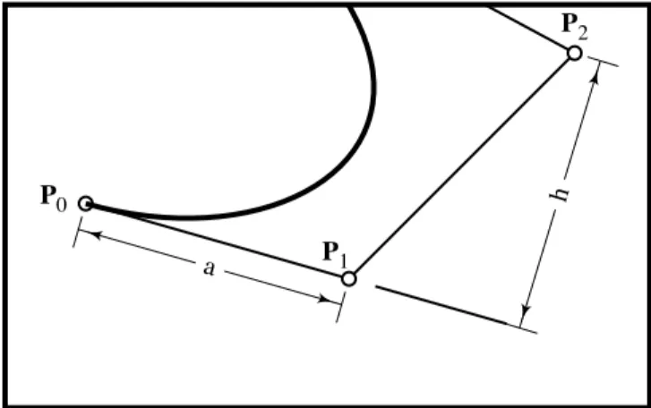
2−p3 and q0−q1 are collinear, but they need not be of equal length. This amounts to saying that they have a common tangent line, though the magnitude of the tangent vector may be different. G2 _{(second order visual} or geometric continuity) means that the two neighboring curves have the same tangent line and also the same curvature at their common boundary. The curvature of a B´ezier curve at its endpoint is given by

κ = n−1 n

h a2

wherenis the degree of the curve andaandhare as shown in Fig. 2.15. Note that ais the length

of the first leg of the control polygon, andhis the perpendicular distance fromP2to the first leg of the control polygon.

Two curves that areGn _{can always be reparameterized so that they are C}n_{. This provides a}

practical definition ofGn _continuity.

2.7

Three Dimensional B´

ezier Curves

It should be obvious that if the control points happen to be defined in three dimensional space, the resulting B´ezier curve is also three dimensional. Such a curve is sometimes called a space curve, and a two dimensional curve is called aplanar curve. Note that since a degree two B´ezier curve is defined using three control points, every degree two curve is planar, even if the control points are in a three dimensional coordinate system.

2.8

Rational B´

ezier Curves

It is possible to change the shape of a B´ezier curve by scaling the blending functions Bn i of the

2.8. RATIONAL B ´EZIER CURVES 23

a

h P₀

P₁

P₂ P₃

Figure 2.15: Endpoint curvature.

is essential for the blending functions to sum to one (or else the curve will change with the coordinate system), we must normalize the blending functions by dividing through by their total value. Thus, the equation becomes

w0Bn0(t)P0 + ... + wnBnn(t)Pn

w0B0n(t) + ... + wnBnn(t)

.

The effect of changing a control point weight is illustrated in Fig. 2.16. This type of curve is known as arational B´ezier curve, because the blending functions are rational polynomials, or the ratioof two polynomials. The B´ezier curves that we have dealt with up to now are sometimes known as non-rationalor integral B´ezier curves. There are more important reasons for using rational B´ezier curves than simply the increased control it provides over the shape of the curve. For example, a perspective drawing of a 3D B´ezier curve (integral or rational) is a rational B´ezier curve. Also, rational B´ezier curves are needed to exactly express all conic sections. A degree two integral B´ezier curve can only represent a parabola. Exact representation of circles requires rational degree two B´ezier curves.

A rational B´ezier curve can be viewed as the projection of a 3-D curve. Fig. 2.17 shows two curves: a 3-D curve and a 2-D curve. The 2-D curve lies on the planez= 1 and it is defined as the

projection of the 3-D curve onto the planez = 1. One way to consider this is to imagine a funny

looking cone whose vertex is at the origin and which contains the 3-D curve. In other words, this cone is the collection of all lines which contain the origin and a point on the curve. Then, the 2-D rational B´ezier curve is the intersection of the cone with the planez= 1.

If the 2-D rational B´ezier curve has control points (xi, yi) with corresponding weightswi, then

the (X, Y, Z) coordinates of the 3-D curve are (xiwi, yiwi, wi). Denote points on the 3-D curve using

upper case variables (X(t), Y(t), Z(t)) and on the 2-D curve using lower case variables (x(t), y(t)).

Then, any point on the 2-D rational B´ezier curve can be computed by computing the corresponding point on the 3-D curve, (X(t), Y(t), Z(t)), and projecting it to the planez= 1 by setting

x(t) =X(t)

Z(t), y(t) = Y(t) Z(t).

P₀ P₁

P₂

P₃ w₂=0

w₂=.5 w₂=1

w₂=2

w₂=5 _w

2=10

Figure 2.16: Rational B´ezier curve.

2.9

Tangency and Curvature

The equations for the endpoint tangency and curvature of a rational B´ezier curve must be computed using the quotient rule for derivatives — it does not work to simply compute the tangent vector and curvature for the three dimensional non-rational B´ezier curve and then project that value to the (x, y) plane. For a degreenrational B´ezier curve,

x(t) = xn(t) d(t) =

w0x0#n₀$(1−t)n+w1x1#n₁$(1−t)n−1t+w2x2#₂n$(1−t)n−2t2+. . .

w0#n₀$(1−t)n+w1#n₁$(1−t)n−1t+w2#n₂$(1−t)n−2t2+. . . ;

y(t) =yn(t) d(t) =

w0y0#n₀$(1−t)n+w1y1#n₁$(1−t)n−1t+w2y2#n₂$(1−t)n−2t2+. . .

w0#n₀$(1−t)n+w1#n₁$(1−t)n−1t+w2#n₂$(1−t)n−2t2+. . .

the equation for the tangent vectort= 0 must be found by evaluating the following equations:

˙

x(0) = d(0) ˙xn(0)−d˙(0)xn(0)

d2₍₀₎ ; y˙(0) =

d(0) ˙yn(0)−d˙(0)yn(0)

d2₍₀₎ from which

P#_{(0) =} w1

w0n

2.9. TANGENCY AND CURVATURE 25

x

y

z

z=1

(

x

,

y

,1)

w

(

x

,

y

,1)

w

(

x

,

y

,1)

w

(

x

,

y

,1)

w

(

x

,

y

,1)

(

x

,

y

,1)

(

x

,

y

,1)

(

x

,

y

,1)

z

x

z=1

_x

i

w

x

w

1

and the curvatureκatt= 0 is found by evaluating the curvature equation κ= |x˙y¨−y˙x¨|

( ˙x2_{+ ˙y}2₎3₂ from which it can be shown

κ(0) = w0w2 w2

1

n₋1 n

h a2 whereaandhare as shown in Figure 2.15.

2.10

Reparametrization

Any integral parametric curve X(t) = (x(t), y(t)) can be reparametrized by the substitution t = f(u). If f(u) = a0 + a1u, then the reparametrization has the effect of changing the range over which the curve segment is defined. Thus, two B´ezier subdivisions can always accomplish exactly what a linear parameter substitution does.

It is also legal forf(u) to be nonlinear. This, of course, does not change the shape of the curve

but it does cause the curve to be improperly parametrized, which means that to each point on the curve there corresponds more than one parameter valueu. There are occasions when it is desirable

to do this. If so, however, it is advisable that the curve does not end up beingmultiply traced, which means that portions of the curve get redrawn as the parameter sweeps from zero to one.

A rational parametric curve can be reparametrized with the substitutiont = f(u)/g(u). In this

case, it is actually possible to perform a rational-linear reparametrization which does not change the endpoints of our curve segment. If we let

t = a(1−u) + bu c(1₋u) + du

and wantu= 0 when t= 0 andu= 1 when t= 1, thena= 0 andb=d. Since we can scale then

numerator and denominator without affecting the reparametrization, setc= 1 and we are left with t = bu

(1₋u) + bu

A rational B´ezier curve

X(t) =

#n

0 $

w0P0(1−t)n + #n₁$w1P1(1−t)n−1t + ... + #n_n$wnPntn

#n

0 $

w0(1₋t)n + #n

1 $

w1(1₋t)n−1_t + _... + #n

n

$

wntn

can be raparametrized without changing its endpoints by making the substitutions

t = bu

(1₋u) + bu, (1−t) =

(1₋u)

(1₋u) + bu.

After multiplying numerator and denominator by ((1₋u) + bu)n, we obtain

X(t) =

#n

0 $₍

b0_w0)P0(1

−t)n ₊ #n

1 $₍

b1_w1)P1(1

−t)n−1_{t + ... +} #n n

$₍

bn_w n)Pntn

#n

0 $

b0_w0(1−t)n ₊ #n

1 $

b1_w1(1−t)n−1_{t + ... +} #n n

$

bn_w ntn

2.11. CIRCULAR ARCS 27

q

P₁; w₁= cosq/2

P₀; w₀= 1

P₂; w₂= 1

d

r

q

Q₁; w₁= (1 + 2cosq/2)/3 Q₀; w₀= 1

Q₂; w₂= (1 + 2cosq/2)/3

Q₃; w₃= 1

e

e

r

Figure 2.18: Circular arcs.

2.11

Circular Arcs

Circular arcs can be exactly represented using rational B´ezier curves. Figure 2.18 shows a circular arc as both a degree two and a degree three rational B´ezier curve. Of course, the control polygons are tangent to the circle. The degree three case is a simple degree elevation of the degree two case. The lengtheis given by

e= 2 sin

θ

2 1 + 2 cosθ

2

r.

The degree two case has trouble when θ approaches 180◦ sinceP1 moves to infinity, although this can be remedied by just using homogeneous coordinates. The degree three case has the advantage that it can represent a larger arc, but even here the length egoes to infinity asθ approaches 240◦_.

For large arcs, a simple solution is to just cut the arc in half and use two cubic B´ezier curves. A complete circle can be represented as a degree five B´ezier curve as shown in Figure 2.19. Here, the

p₀ = (0,0) p₁ = (4,0) p₂ = (2,4)

p₃ = (-2,4)

p₄ = (-4,0) p₅ = (0,0)

Figure 2.19: Circle as Degree 5 Rational B´ezier Curve. weights arew0=w5= 1 andw1=w2=w3=w4=1₅.

2.12

Explicit B´

ezier Curves

An explicit B´ezier curve is one for which the x-coordinates of the control points are evenly spaced

between 0 and 1. That is,Pi= (_ni, yi), i= 0, . . . , n. Since &ni=0 niB n

i(t)≡t[(1−t) +t]n ≡t, such

a B´ezier curve takes on the important special form

x = t y = f(t)

or simply

y=f(x).

An explicit B´ezier curve is sometimes called a non-parametric B´ezier curve. It is just a polynomial function expressed in the Bernstein polynomial basis. Figure 2.20 shows a degree five explicit B´ezier curve.

P

P

P

P

P

P

0 .2 .4 .6 .8 1

Figure 2.20: Explicit B´ezier curve.

2.13

Integrating Bernstein polynomials

Recall that the hodograph (first derivative) of a B´ezier curve is easily found by simply differencing adjacent control points (Section 2.5). It is equally simple to compute the integral of a Bernstein polynomial. Since the integral of a polynomial in Bernstein form

p(t) =

n

%

i=0

piBin(t) (2.4)

is that polynomial whose derivative is p(t). If the desired integral is a degreen+ 1 polynomial in

Bernstein form

q(t) =

n+1 %

i=0

2.14. FORWARD DIFFERENCING 29

we have

pi= (n+ 1)(qi+1−qi). (2.6)

Hence,q0= 0 and

qi=

&i−1

j=0pj

n+ 1 , i= 1, n+ 1. (2.7)

Note that ifp(t) is expressed as an explicit B´ezier curve,q(t) can be interpreted as the area under p(t) between the linesx= 0 andx=t. Thus, the entire area under an explicit B´ezier curve can be

computed as simply the average of the control points! This is so because

q(1) =qn+1= &n

j=0pj

n+ 1 . (2.8)

2.14

Forward Differencing

Horner’s algorithm is the fastest method for evaluating a polynomial at a single point. For a degree

npolynomial, it requiresnmultiplies andnadds.

If a polynomial is to be evaluated at several evenly spaced valuest, t+δ, t+ 2δ, . . . , t+kδ, the

fastest method is to useforward differences. Consider a degree 1 polynomial

f(t) =a0+a1t. The difference between two adjacent function values is

∆1(t) =f(t+δ)₋f(t) = [a0+a1(t+δ)]−[a0+a1t] =a1δ. Thus,f(t) can be evaluated at several evenly spaced points using the algorithm:

∆1=a1δ

t0= 0

f(0) =a0

for i= 1 to k do ti=ti−1+δ

f(ti) =f(ti−1) + ∆1

endfor

Thus, each successive evaluation requires only one add, as opposed to one add and one multiply for Horner’s algorithm.

This idea extends to polynomials of any degree. For the quadratic case,

f(t) =a0+a1t+a2t2. The difference between two adjacent function values is

∆1(t) =f(t+δ)₋f(t) = [a0+a1(t+δ) +a2(t+δ)2]−[a0+a1t+a2t2] ∆1(t) =a1δ+a2δ2+ 2a2tδ.

t0= 0

f(0) =a0

for i= 1 to k do ti=ti−1+δ

∆1(ti) =a1δ+a2δ2+ 2a2ti−1δ

f(ti) =f(ti−1) + ∆1(ti−1)

endfor

In this case, ∆(t) is a linear polynomial, so we can evaluate it as above, by defining

∆2(t) = ∆1(t+δ)₋∆1(t) = 2a2δ2 and our algorithm now becomes

t0= 0

f(0) =a0 ∆1=a1δ+a2δ2 ∆2= 2a2δ2

for i= 1 to k do ti=ti−1+δ

f(ti) =f(ti−1) + ∆1

∆1= ∆1+ ∆2

endfor

It should be clear that for a degreenpolynomial, each successive evaluation requiresnadds and no

multiplies! For a cubic polynomial

f(t) =a0+a1t+a2t2+a3t3, the forward difference algorithm becomes

t0= 0

f(0) =a0

∆1=a1δ+a2δ2+a3δ3 ∆2= 2a2δ2+ 6a3δ3 ∆3= 6a3δ3

for i= 1 to k do ti=ti−1+δ

f(ti) =f(ti−1) + ∆1

∆1= ∆1+ ∆2 ∆2= ∆2+ ∆3

2.14. FORWARD DIFFERENCING 31

Several questions remain. First, what are the initial values for the ∆i if we want to start at

some value other thant = 0. Second, what is a general equation for the ∆i for a general degreen

polynomialf(t). Also, what if our polynomial is not in power basis.

These questions can be answered almost trivially by observing the following. Sinceti+1=ti+δ,

we have

∆1(ti) =f(ti+1)−f(t);

∆j(ti) = ∆j−1(ti+1)−∆j−1(ti), j= 2, . . . , n;

∆n(ti) = ∆n(ti+1) = ∆n(ti+k) = a constant

∆n+1= 0

Thus, our initial values for ∆j(ti) can be found by simply computingf(ti), f(ti+1), . . . , f(ti+n)

and from them computing the initial differences. This lends itself nicely to a table. Here is the table for a degree four case:

f(ti) f(ti+1) f(ti+2) f(ti+3) f(ti+4)

∆1(ti) ∆1(ti+1) ∆1(ti+2) ∆1(ti+3)

∆2(ti) ∆2(ti+1) ∆2(ti+2)

∆3(ti) ∆3(ti+1)

∆4(ti)

0 0 0 0 0

To compute f(ti+5), we simply note that every number R in this table, along with its right hand

neighborRrightand the number directly beneath it Rdownobey the rule

Rright=R+Rdown.

Thus, we can simply fill in the values

∆4(ti+1) = ∆4(ti) + 0

∆3(ti+2) = ∆3(ti+1) + ∆4(ti+1)

∆2(ti+3) = ∆2(ti+2) + ∆3(ti+2)

∆1(ti+4) = ∆1(ti+3) + ∆2(ti+3)

f(ti+5) =f(ti+4) + ∆1(ti+4)

Note that this technique is independent of the basis in whichf(t) is defined. Thus, even if it

is defined in Bernstein basis, all we need to do is to evaluate itn+ 1 times to initiate the forward

differencing.

For example, consider the degree 4 polynomial for whichf(ti) = 1,f(ti+1) = 3, f(ti+2) = 2,

f(ti+3) = 5, f(ti+4) = 4. We can compute f(ti+5) = −24, f(ti+6) = −117, and f(ti+7) = −328

from the following difference table:

t: ti ti+1 ti+2 ti+3 ti+4 ti+5 ti+6 ti+7

f(t) : 1 3 2 5 4 ₋24 ₋117 ₋328

∆1(t) : 2 ₋1 3 ₋1 ₋28 ₋93 ₋211

∆2(t) : ₋3 4 ₋4 ₋27 ₋65 ₋118

∆3(t) : 7 ₋8 ₋23 ₋38 ₋53

∆4(t) : −15 −15 −15 −15 −15

2.15

Forward Differencing

Horner’s algorithm is the fastest method for evaluating a polynomial at a single point. For a degree

npolynomial, it requiresnmultiplies andnadds.

If a polynomial is to be evaluated at several evenly spaced valuest, t+δ, t+ 2δ, . . . , t+kδ, the

fastest method is to useforward differences. Consider a degree 1 polynomial

f(t) =a0+a1t. The difference between two adjacent function values is

∆1(t) =f(t+δ)₋f(t) = [a0+a1(t+δ)]−[a0+a1t] =a1δ. Thus,f(t) can be evaluated at several evenly spaced points using the algorithm:

∆1=a1δ

t0= 0

f(0) =a0

for i= 1 to k do

ti=ti−1+δ

f(ti) =f(ti−1) + ∆1

endfor

Thus, each successive evaluation requires only one add, as opposed to one add and one multiply for Horner’s algorithm.

This idea extends to polynomials of any degree. For the quadratic case,

f(t) =a0+a1t+a2t2. The difference between two adjacent function values is

∆1(t) =f(t+δ)₋f(t) = [a0+a1(t+δ) +a2(t+δ)2]−[a0+a1t+a2t2] ∆1(t) =a1δ+a2δ2+ 2a2tδ.

We can now write

t0= 0

f(0) =a0

for i= 1 to k do ti=ti−1+δ

∆1(ti) =a1δ+a2δ2+ 2a2ti−1δ

f(ti) =f(ti−1) + ∆1(ti−1)

endfor

In this case, ∆(t) is a linear polynomial, so we can evaluate it as above, by defining

∆2(t) = ∆1(t+δ)₋∆1(t) = 2a2δ2 and our algorithm now becomes

2.15. FORWARD DIFFERENCING 33 t0= 0

f(0) =a0 ∆1=a1δ+a2δ2 ∆2= 2a2δ2

for i= 1 to k do ti=ti−1+δ

f(ti) =f(ti−1) + ∆1

∆1= ∆1+ ∆2

endfor

It should be clear that for a degreenpolynomial, each successive evaluation requiresnadds and no

multiplies! For a cubic polynomial

f(t) =a0+a1t+a2t2+a3t3, the forward difference algorithm becomes

t0= 0

f(0) =a0

∆1=a1δ+a2δ2+a3δ3 ∆2= 2a2δ2+ 6a3δ3 ∆3= 6a3δ3

for i= 1 to k do ti=ti−1+δ

f(ti) =f(ti−1) + ∆1

∆1= ∆1+ ∆2 ∆2= ∆2+ ∆3

endfor

Several questions remain. First, what are the initial values for the ∆i if we want to start at

some value other thant = 0. Second, what is a general equation for the ∆i for a general degreen

polynomialf(t). Also, what if our polynomial is not in power basis.

These questions can be answered almost trivially by observing the following. Sinceti+1=ti+δ,

we have

∆1(ti) =f(ti+1)−f(t);

∆j(ti) = ∆j−1(ti+1)−∆j−1(ti), j= 2, . . . , n;

∆n(ti) = ∆n(ti+1) = ∆n(ti+k) = a constant

Thus, our initial values for ∆j(ti) can be found by simply computingf(ti), f(ti+1), . . . , f(ti+n)

and from them computing the initial differences. This lends itself nicely to a table. Here is the table for a degree four case:

f(ti) f(ti+1) f(ti+2) f(ti+3) f(ti+4)

∆1(ti) ∆1(ti+1) ∆1(ti+2) ∆1(ti+3)

∆2(ti) ∆2(ti+1) ∆2(ti+2)

∆3(ti) ∆3(ti+1)

∆4(ti)

0 0 0 0 0

To compute f(ti+5), we simply note that every number R in this table, along with its right hand

neighborRrightand the number directly beneath it Rdownobey the rule

Rright=R+Rdown.

Thus, we can simply fill in the values

∆4(ti+1) = ∆4(ti) + 0

∆3(ti+2) = ∆3(ti+1) + ∆4(ti+1)

∆2(ti+3) = ∆2(ti+2) + ∆3(ti+2)

∆1(ti+4) = ∆1(ti+3) + ∆2(ti+3)

f(ti+5) =f(ti+4) + ∆1(ti+4)

Note that this technique is independent of the basis in whichf(t) is defined. Thus, even if it

is defined in Bernstein basis, all we need to do is to evaluate itn+ 1 times to initiate the forward

differencing.

For example, consider the degree 4 polynomial for whichf(ti) = 1,f(ti+1) = 3, f(ti+2) = 2,

f(ti+3) = 5, f(ti+4) = 4. We can compute f(ti+5) = −24, f(ti+6) = −117, and f(ti+7) = −328

from the following difference table:

t: ti ti+1 ti+2 ti+3 ti+4 ti+5 ti+6 ti+7

f(t) : 1 3 2 5 4 ₋24 ₋117 ₋328

∆1(t) : 2 ₋1 3 ₋1 ₋28 ₋93 ₋211

∆2(t) : ₋3 4 ₋4 ₋27 ₋65 ₋118

∆3(t) : 7 ₋8 ₋23 ₋38 ₋53

∆4(t) : ₋15 ₋15 ₋15 ₋15 ₋15