A Tutorial on
Uppaal
4.0
Updated November 28, 2006Gerd Behrmann, Alexandre David, and Kim G. Larsen Department of Computer Science, Aalborg University, Denmark
{behrmann,adavid,kgl}@cs.auc.dk.
Abstract. This is a tutorial paper on the toolUppaal. Its goal is to be
a short introduction on the flavour of timed automata implemented in the tool, to present its interface, and to explain how to use the tool. The contribution of the paper is to provide reference examples and modelling patterns.
1
Introduction
Uppaal is a toolbox for verification of real-time systems jointly developed by Uppsala University and Aalborg University. It has been applied successfully in case studies ranging from communication protocols to multimedia applications [35,55,24,23,34,43,54,44,30]. The tool is designed to verify systems that can be modelled as networks of timed automata extended with integer variables, struc-tured data types, user defined functions, and channel synchronisation.
The first version ofUppaalwas released in 1995 [52]. Since then it has been in constant development [21,5,13,10,26,27]. Experiments and improvements in-clude data structures [53], partial order reduction [20], a distributed version of Uppaal [17,9], guided and minimal cost reachability [15,51,16], work on UML Statecharts [29], acceleration techniques [38], and new data structures and memory reductions [18,14]. Version 4.0 [12] brings symmetry reduction [36], the generalised sweep-line method [49], new abstraction techniques [11], priori-ties [28], and user defined functions to the mainstream. Uppaalhas also gen-erated related Ph.D. theses [50,57,45,56,19,25,32,8,31]. It features a Java user interface and a verification engine written in C++ . It is freely available at http://www.uppaal.com/.
This tutorial covers networks of timed automata and the flavour of timed automata used inUppaalin section 2. The tool itself is described in section 3, and three extensive examples are covered in sections 4, 5, and 6. Finally, section 7 introduces common modelling patterns often used withUppaal.
2
Timed Automata in Uppaal
The model-checkerUppaalis based on the theory of timed automata [4] (see [42] for automata theory) and its modelling language offers additional features such as bounded integer variables and urgency. The query language of Uppaal, used
to specify properties to be checked, is a subset of TCTL (timed computation tree logic) [39,3]. In this section we present the modelling and the query languages of Uppaaland we give an intuitive explanation of time in timed automata. 2.1 The Modelling Language
Networks of Timed Automata A timed automaton is a finite-state machine extended with clock variables. It uses a dense-time model where a clock variable evaluates to a real number. All the clocks progress synchronously. In Uppaal, a system is modelled as a network of several such timed automata in parallel. The model is further extended with bounded discrete variables that are part of the state. These variables are used as in programming languages: They are read, written, and are subject to common arithmetic operations. A state of the system is defined by the locations of all automata, the clock values, and the values of the discrete variables. Every automaton may fire an edge (sometimes misleadingly called a transition) separately or synchronise with another automaton1
, which leads to a new state.
Figure 1(a) shows a timed automaton modelling a simple lamp. The lamp has three locations: off, low, and bright. If the user presses a button, i.e., synchronises with press?, then the lamp is turned on. If the user presses the button again, the lamp is turned off. However, if the user is fast and rapidly presses the button twice, the lamp is turned on and becomes bright. The user model is shown in Fig. 1(b). The user can press the button randomly at any time or even not press the button at all. The clocky of the lamp is used to detect if the user was fast (y <5) or slow (y >= 5).
off low bright
press? y:=0
y>=5 press?
press? y<5
press?
‚ ‚ ‚ ‚ ‚
idle
press!
(a) Lamp. (b) User.
Fig. 1.The simple lamp example.
We give the basic definitions of the syntax and semantics for the basic timed automata. In the following we will skip the richer flavour of timed automata supported inUppaal, i.e., with integer variables and the extensions of urgent and committed locations. For additional information, please refer to the help
1
or several automata in case of broadcast synchronisation, another extension of timed automata inUppaal.
menu inside the tool. We use the following notations: C is a set of clocks and
B(C) is the set of conjunctions over simple conditions of the form x ⊲⊳ c or
x−y ⊲⊳ c, wherex, y ∈C,c∈Nand⊲⊳∈ {<,≤,=,≥, >}. A timed automaton is a finite directed graph annotated with conditions over and resets of non-negative real valued clocks.
Definition 1 (Timed Automaton (TA)). A timed automaton is a tuple (L, l0, C, A, E, I), where L is a set of locations, l0 ∈ L is the initial location,
C is the set of clocks,Ais a set of actions, co-actions and the internalτ-action,
E⊆L×A×B(C)×2C×Lis a set of edges between locations with an action, a guard and a set of clocks to be reset, and I:L→B(C) assigns invariants to
locations.
In the previous example on Fig. 1,y:=0is the reset of the clocky, and the labels press?andpress!denote action–co-action (channel synchronisations here).
We now define the semantics of a timed automaton. A clock valuation is a functionu:C→R≥0 from the set of clocks to the non-negative reals. Let RC be the set of all clock valuations. Letu0(x) = 0 for allx∈C. We will abuse the notation by considering guards and invariants as sets of clock valuations, writing
u∈I(l) to mean thatusatisfiesI(l).
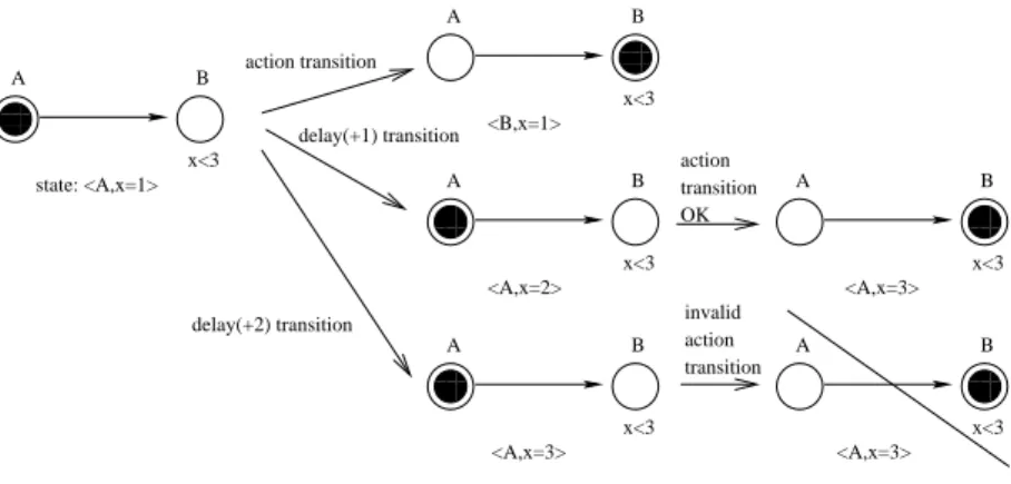
000 000 000 111 111 111000000111111 B A x<3 000 000 000 111 111 111000000111111 B A x<3 000 000 000 111 111 111000000111111 B A x<3 000 000 000 111 111 111 000000 111111 A B x<3 000 000 000 111 111 111 000000 111111 A B x<3 000 000 000 111 111 111 000000 111111 00000000 00000000 00000000 00000000 00000000 00000000 11111111 11111111 11111111 11111111 11111111 11111111 0000000 0000000 0000000 0000000 0000000 0000000 0000000 0000000 1111111 1111111 1111111 1111111 1111111 1111111 1111111 1111111 0000000 0000000 0000000 0000000 0000000 0000000 0000000 0000000 0000000 0000000 0000000 0000000 0000000 0000000 0000000 0000000 0000000 0000000 0000000 0000000 0000000 0000000 1111111 1111111 1111111 1111111 1111111 1111111 1111111 1111111 1111111 1111111 1111111 1111111 1111111 1111111 1111111 1111111 1111111 1111111 1111111 1111111 1111111 1111111 0000 1111 0000 1111 00000000000 00000000000 00000000000 00000000000 00000000000 00000000000 00000000000 00000000000 00000000000 00000000000 00000000000 00000000000 00000000000 00000000000 00000000000 00000000000 11111111111 11111111111 11111111111 11111111111 11111111111 11111111111 11111111111 11111111111 11111111111 11111111111 11111111111 11111111111 11111111111 11111111111 11111111111 11111111111 B A x<3 <B,x=1> <A,x=2> <A,x=3> <A,x=3> <A,x=3> action transition delay(+1) transition delay(+2) transition state: <A,x=1> action transition OK invalid action transition
invalid state: invariant x<3 violated
Fig. 2.Semantics of TA: different transitions from a given initial state.
Definition 2 (Semantics of TA).Let(L, l0, C, A, E, I)be a timed automaton. The semantics is defined as a labelled transition systemhS, s0,→i, whereS⊆L× RCis the set of states,s
0= (l0, u0)is the initial state, and→⊆S×(R≥0∪A)×S is the transition relation such that:
– (l, u)−→d (l, u+d)if ∀d′: 0≤d′≤d =⇒ u+d′∈I(l), and – (l, u)−→a (l′, u′)if there existse= (l, a, g, r, l′)∈E s.t.u∈g,
where for d ∈ R≥0, u+d maps each clock x in C to the value u(x) +d, and [r7→0]udenotes the clock valuation which maps each clock inrto 0 and agrees
with uoverC\r.
Figure 2 illustrates the semantics of TA. From a given initial state, we can choose to take anaction or a delay transition (different values here). Depending of the chosen delay, further actions may be forbidden.
Timed automata are often composed into anetwork of timed automata over a common set of clocks and actions, consisting of n timed automata Ai = (Li, li0, C, A, Ei, Ii), 1 ≤ i ≤ n. A location vector is a vector ¯l = (l1, . . . , ln). We compose the invariant functions into a common function over location vec-torsI(¯l) =∧iIi(li). We write ¯l[l′i/li] to denote the vector where theith element
li of ¯l is replaced byli′. In the following we define the semantics of a network of timed automata.
Definition 3 (Semantics of a network of Timed Automata). Let Ai = (Li, li0, C, A, Ei, Ii)be a network ofntimed automata. Let¯l0= (l10, . . . , l
0 n)be the initial location vector. The semantics is defined as a transition systemhS, s0,→i, where S = (L1× · · · ×Ln)×RC is the set of states, s0= (¯l0, u0) is the initial state, and →⊆S×S is the transition relation defined by:
– (¯l, u)−→d (¯l, u+d)if ∀d′: 0≤d′≤d =⇒ u+d′∈I(¯l). – (¯l, u)−→a (¯l[l′
i/li], u′)if there exists li τ gr
−−→l′
i s.t.u∈g,
u′= [r7→0]uandu′∈I(¯l[l′ i/li]). – (¯l, u)−→a (¯l[l′
j/lj, li′/li], u′)if there existli c?giri
−−−−→l′ i and
lj c!gjrj
−−−−→l′
j s.t. u∈(gi∧gj),u′ = [ri∪rj 7→0]uandu′∈I(¯l[lj′/lj, l′i/li]). As an example of the semantics, the lamp in Fig. 1 may have the follow-ing states (we skip the user): (Lamp.off, y = 0) → (Lamp.off, y = 3) →
(Lamp.low, y = 0) → (Lamp.low, y = 0.5) → (Lamp.bright, y = 0.5) →
(Lamp.bright, y= 1000) . . .
Timed Automata in Uppaal TheUppaalmodelling language extends timed automata with the following additional features (see Fig. 3:
Templates automata are defined with a set of parameters that can be of any type (e.g.,int,chan). These parameters are substituted for a given argument in the process declaration.
Constants are declared asconst name value. Constants by definition cannot be modified and must have an integer value.
Bounded integer variables are declared asint[min,max] name, wheremin andmaxare the lower and upper bound, respectively. Guards, invariants, and assignments may contain expressions ranging over bounded integer variables. The bounds are checked upon verification and violating a bound leads to an invalid state that is discarded (at run-time). If the bounds are omitted, the default range of -32768 to 32768 is used.
Fig. 3.Declarations of a constant and a variable, and illustration of some of the channel synchronisations between two templates of the train gate example of Section 4, and some committed locations.
Binary synchronisation channels are declared as chan c. An edge labelled with c! synchronises with another labelled c?. A synchronisation pair is chosen non-deterministically if several combinations are enabled.
Broadcast channels are declared as broadcast chan c. In a broadcast syn-chronisation one sender c! can synchronise with an arbitrary number of receiversc?. Any receiver than can synchronise in the current state must do so. If there are no receivers, then the sender can still execute thec!action, i.e. broadcast sending is never blocking.
Urgent synchronisation channels are declared by prefixing the channel decla-ration with the keywordurgent. Delays must not occur if a synchronisation transition on an urgent channel is enabled. Edges using urgent channels for synchronisation cannot have time constraints, i.e., no clock guards.
Urgent locations are semantically equivalent to adding an extra clockx, that is reset on all incoming edges, and having an invariantx<=0on the location. Hence, time is not allowed to pass when the system is in an urgent location. Committed locations are even more restrictive on the execution than urgent locations. A state is committed if any of the locations in the state is commit-ted. A committed state cannot delay and the next transition must involve an outgoing edge of at least one of the committed locations.
Arrays are allowed for clocks, channels, constants and integer variables. They are defined by appending a size to the variable name, e.g.chan c[4]; clock a[2]; int[3,5] u[7];.
Initialisers are used to initialise integer variables and arrays of integer vari-ables. For instance,int i = 2; orint i[3] = {1, 2, 3};.
Record types are declared with thestructconstruct like in C.
Custom types are defined with the C-like typedef construct. You can define any custom-type from other basic types such as records.
User functions are defined either globally or locally to templates. Template parameters are accessible from local functions. The syntax is similar to C except that there is no pointer. C++ syntax for references is supported for the arguments only.
Expressions in Uppaal Expressions inUppaalrange over clocks and integer variables. The BNF is given in Fig. 33 in the appendix. Expressions are used with the following labels:
Select A select label contains a comma separated list ofname : typeexpressions wherenameis a variable name andtypeis a defined type (built-in or custom). These variables are accessible on the associated edge only and they will take a non-deterministic value in the range of their respective types.
Guard A guard is a particular expression satisfying the following conditions: it is side-effect free; it evaluates to a boolean; only clocks, integer variables, and constants are referenced (or arrays of these types); clocks and clock differences are only compared to integer expressions; guards over clocks are essentially conjunctions (disjunctions are allowed over integer conditions). A guard may call a side-effect free function that returns a bool, although clock constraints are not supported in such functions.
Synchronisation A synchronisation label is either on the form Expression! orExpression?or is an empty label. The expression must be side-effect free, evaluate to a channel, and only refer to integers, constants and channels. Update An update label is a comma separated list of expressions with a
side-effect; expressions must only refer to clocks, integer variables, and constants and only assign integer values to clocks. They may also call functions. Invariant An invariant is an expression that satisfies the following conditions: it
is side-effect free; only clock, integer variables, and constants are referenced; it is a conjunction of conditions of the formx<eor x<=ewherexis a clock reference andeevaluates to an integer. An invariant may call a side-effect free function that returns a bool, although clock constraints are not supported in such functions.
2.2 The Query Language
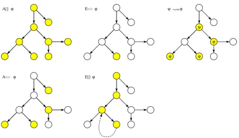
The main purpose of a model-checker is verify the model w.r.t. a requirement specification. Like the model, the requirement specification must be expressed in a formally well-defined and machine readable language. Several such logics exist in the scientific literature, andUppaaluses a simplified version of TCTL. Like in TCTL, the query language consists of path formulae and state formulae.2 State formulae describe individual states, whereas path formulae quantify over paths or traces of the model. Path formulae can be classified into reachability, safety andliveness. Figure 4 illustrates the different path formulae supported by Uppaal. Each type is described below.
State Formulae A state formula is an expression (see Fig. 33) that can be evaluated for a state without looking at the behaviour of the model. For instance, this could be a simple expression, likei == 7, that is true in a state whenever
i equals 7. The syntax of state formulae is a superset of that of guards, i.e., a state formula is a side-effect free expression, but in contrast to guards, the use of disjunctions is not restricted. It is also possible to test whether a particular process is in a given location using an expression on the formP.l, wherePis a process andlis a location.
In Uppaal, deadlock is expressed using a special state formula (although this is not strictly a state formula). The formula simply consists of the keyword deadlock and is satisfied for all deadlock states. A state is a deadlock state if there are no outgoing action transitions neither from the state itself or any of its delay successors. Due to current limitations in Uppaal, the deadlock state formula can only be used with reachability and invariantly path formulae (see below).
Reachability Properties Reachability properties are the simplest form of properties. They ask whether a given state formula,ϕ,possibly can be satisfied
2
A[]ϕ
A<> ϕ
E<>ϕ
E[]ϕ
ψ
ϕ ϕ
ϕ
ψ ϕ
Fig. 4. Path formulae supported in Uppaal. The filled states are those for which a
given state formulae φ holds. Bold edges are used to show the paths the formulae evaluate on.
by any reachable state. Another way of stating this is: Does there exist a path starting at the initial state, such thatϕis eventually satisfied along that path.
Reachability properties are often used while designing a model to perform sanity checks. For instance, when creating a model of a communication protocol involving a sender and a receiver, it makes sense to ask whether it is possible for the sender to send a message at all or whether a message can possibly be received. These properties do not by themselves guarantee the correctness of the protocol (i.e. that any message is eventually delivered), but they validate the basic behaviour of the model.
We express that some state satisfyingϕshould be reachable using the path formulaE3ϕ. InUppaal, we write this property using the syntax E<> ϕ.
Safety Properties Safety properties are on the form: “something bad will never happen”. For instance, in a model of a nuclear power plant, a safety property might be, that the operating temperature is always (invariantly) under a certain threshold, or that a meltdown never occurs. A variation of this property is that “something will possibly never happen”. For instance when playing a game, a safe state is one in which we can still win the game, hence we will possibly not loose.
InUppaalthese properties are formulated positively, e.g., something good is invariantly true. Letϕbe a state formulae. We express thatϕshould be true in all reachable states with the path formulae Aϕ,3
whereasEϕsays that
3
there should exist a maximal path such that ϕis always true.4 InUppaal we writeA[] ϕandE[] ϕ, respectively.
Liveness Properties Liveness properties are of the form: something will even-tually happen, e.g. when pressing the on button of the remote control of the television, then eventually the television should turn on. Or in a model of a communication protocol, any message that has been sent should eventually be received.
In its simple form, liveness is expressed with the path formulaA3ϕ, mean-ing ϕis eventually satisfied.5
The more useful form is the leads to or response property, writtenϕ ψwhich is read as wheneverϕis satisfied, then eventu-allyψ will be satisfied, e.g. whenever a message is sent, then eventually it will be received.6
InUppaal these properties are written asA<> ϕand ϕ --> ψ, respectively.
2.3 Understanding Time
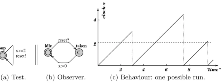
Invariants and Guards Uppaaluses a continuous time model. We illustrate the concept of time with a simple example that makes use of anobserver. Nor-mally an observer is an add-on automaton in charge of detecting events without changing the observed system. In our case the clock reset (x:=0) is delegated to the observer for illustration purposes.
Figure 5 shows the first model with its observer. We have two automata in parallel. The first automaton has a self-loop guarded by x>=2, x being a clock, that synchronises on the channelresetwith the second automaton. The second automaton, the observer, detects when the self loop edge is taken with the location taken and then has an edge going back to idle that resets the clockx. We moved the reset of xfrom the self loop to the observer only to test what happens on the transition before the reset. Notice that the locationtaken is committed (markedc) to avoid delay in that location.
The following properties can be verified in Uppaal (see section 3 for an overview of the interface). Assuming we name the observer automatonObs, we have:
– A[] Obs.taken imply x>=2: all resets off x will happen whenx is above 2. This query means that for all reachable states, being in the location Obs.takenimplies thatx>=2.
– E<> Obs.idle and x>3: this property requires, that it is possible to reach-able state whereObsis in the locationidleandxis bigger than 3. Essentially we check that we may delay at least 3 time units between resets. The result would have been the same for larger values like 30000, since there are no invariants in this model.
4
A maximal path is a path that is either infinite or where the last state has no outgoing transitions.
5
Notice thatA3ϕ=¬E¬ϕ.
6
loop x>=2 reset!
‚ ‚ ‚ ‚ ‚
idle taken
reset?
x:=0
2 4 6 8
2 4
"time"
clock x
(a) Test. (b) Observer. (c) Behaviour: one possible run. Fig. 5.First example with an observer.
loop
x<=3 x>=2 reset!
2 4 6 8
2 4
"time"
clock x
(a) Test. (b) Updated behaviour with an invariant.
Fig. 6.Updated example with an invariant. The observer is the same as in Fig. 5 and is not shown here.
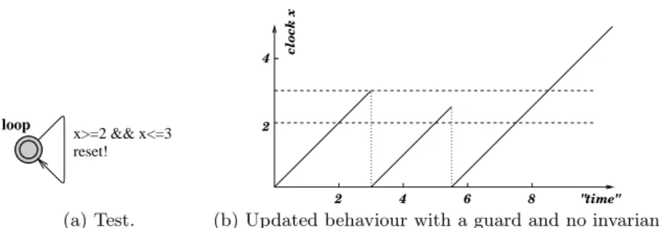
We update the first model and add aninvariant to the locationloop, as shown in Fig. 6. The invariant is a progress condition: the system is not allowed to stay in the state more than 3 time units, so that the transition has to be taken and the clock reset in our example. Now the clock xhas 3 as an upper bound. The following properties hold:
– A[] Obs.taken imply (x>=2 and x<=3)shows that the transition is taken whenxis between 2 and 3, i.e., after a delay between 2 and 3.
– E<> Obs.idle and x>2: it is possible to take the transition whenxis be-tween 2 and 3. The upper bound 3 is checked with the next property. – A[] Obs.idle imply x<=3: to show that the upper bound is respected. The former propertyE<> Obs.idle and x>3no longer holds.
Now, if we remove the invariant and change the guard to x>=2 and x<=3, you may think that it is the same as before, but it is not! The system has no progress condition, just a new condition on the guard. Figure 7 shows what happens: the system may take the same transitions as before, but deadlock may also occur. The system may be stuck if it does not take the transition after 3 time units. In fact, the system fails the property A[] not deadlock. The property A[] Obs.idle imply x<=3does not hold any longer and the deadlock can also be illustrated by the propertyA[] x>3 imply not Obs.taken, i.e., after 3 time units, the transition is not taken any more.
loop
x>=2 && x<=3 reset!
2 4 6 8
2 4
"time"
clock x
(a) Test. (b) Updated behaviour with a guard and no invariant. Fig. 7.Updated example with a guard and no invariant.
P0
S0 S1 S2
x:=0
P1
S0 S1 S2
x:=0
P2
S0 S1 S2
Fig. 8.Automata in parallel with normal, urgent and commit states. The clocks are local, i.e.,P0.xandP1.xare two different clocks.
Committed and Urgent Locations There are three different types of loca-tions inUppaal: normal locations with or without invariants (e.g.,x<=3in the previous example), urgent locations, and committed locations. Figure 8 shows 3 automata to illustrate the difference. The location marked uis urgent and the one marked cis committed. The clocks are local to the automata, i.e.,xin P0 is different fromxin P1.
To understand the difference between normal locations and urgent locations, we can observe that the following properties hold:
– E<> P0.S1 and P0.x>0: it is possible to wait inS1of P0. – A[] P1.S1 imply P1.x==0: it is not possible to wait inS1of P1.
An urgent location is equivalent to a location with incoming edges reseting a designated clockyand labelled with the invarianty<=0. Time may not progress in an urgent state, but interleavings with normal states are allowed.
A committed location is more restrictive: in all the states where P2.S1 is active (in our example), the only possible transition is the one that fires the edge outgoing fromP2.S1. Astatehaving a committed location active is said to
be committed: delay is not allowed and the committed location must be left in the successor state (or one of the committed locations if there are several ones).
3
Overview of the Uppaal Toolkit
Uppaaluses a client-server architecture, splitting the tool into a graphical user interface and a model checking engine. The user interface, or client, is imple-mented in Java and the engine, or server, is compiled for different platforms (Linux, Windows, Solaris).7 As the names suggest, these two components may be run on different machines as they communicate with each other via TCP/IP. There is also a stand-alone version of the engine that can be used on the com-mand line.
3.1 The Java Client
The idea behind the tool is to model a system with timed automata using a graphical editor, simulate it to validate that it behaves as intended, and finally to verify that it is correct with respect to a set of properties. The graphical interface (GUI) of the Java client reflects this idea and is divided into three main parts: the editor, the simulator, and the verifier, accessible via three “tabs”. The Editor A system is defined as a network of timed automata, called pro-cesses in the tool, put in parallel. A process is instantiated from a parameterised template. The editor is divided into two parts: a tree pane to access the different templates and declarations and a drawing canvas/text editor. Figure 9 shows the editor with the train gate example of section 4. Locations are labelled with names and invariants and edges are labelled with guard conditions (e.g.,e==id), synchronisations (e.g.,go?), and assignments (e.g.,x:=0).
The tree on the left hand side gives access to different parts of the system description:
Global declaration Contains global integer variables, clocks, synchronisation channels, and constants.
Templates Train,Gate, andIntQueue are different parameterised timed au-tomata. A template may have local declarations of variables, channels, and constants.
Process assignments Templates are instantiated into processes. The process assignment section contains declarations for these instances.
System definition The list of processes in the system.
The syntax used in the labels and the declarations is described in the help system of the tool. The local and global declarations are shown in Fig. 10. The graphical syntax is directly inspired from the description of timed automata in section 2.
Fig. 9.The train automaton of the train gate example. Theselect button is activated in the tool-bar. In this mode the user can move locations and edges or edit labels. The other modes are for adding locations, edges, and vertices on edges (called nails). A new location has no name by default. Two text fields allow the user to define the template name and its parameters. Useful trick: The middle mouse button is a shortcut for adding new elements, i.e. pressing it on the canvas, a location, or edge adds a new location, edge, or nail, respectively.
The Simulator The simulator can be used in three ways: the user can run the system manually and choose which transitions to take, the random mode can be toggled to let the system run on its own, or the user can go through a trace (saved or imported from the verifier) to see how certain states are reachable. Figure 11 shows the simulator. It is divided into four parts:
The control part is used to choose and fire enabled transitions, go through a trace, and toggle the random simulation.
The variable view shows the values of the integer variables and the clock con-straints.Uppaal does not show concrete states with actual values for the clocks. Since there are infinitely many of such states,Uppaalinstead shows sets of concrete states known as symbolic states. All concrete states in a sym-bolic state share the same location vector and the same values for discrete variables. The possible values of the clocks is described by a set of
con-7
Fig. 10. The different local and global declarations of the train gate example. We superpose several screen-shots of the tool to show the declarations in a compact manner.
straints. The clock validation in the symbolic state are exactly those that satisfy all constraints.
The system view shows all instantiated automata and active locations of the current state.
The message sequence chart shows the synchronisations between the differ-ent processes as well as the active locations at every step.
The Verifier The verifier “tab” is shown in Fig. 12. Properties are selectable in theOverview list. The user may model-check one or several properties,8 insert or remove properties, and toggle the view to see the properties or the comments in the list. When a property is selected, it is possible to edit its definition (e.g., E<> Train1.Cross and Train2.Stop. . . ) or comments to document what the property means informally. TheStatus panel at the bottom shows the commu-nication with the server.
When trace generation is enabled and the model-checker finds a trace, the user is asked if she wants to import it into the simulator. Satisfied properties are marked green and violated ones red. In case either an over approximation or an under approximation has been selected in the options menu, then it may happen that the verification is inconclusive with the approximation used. In that case the properties are marked yellow.
8
Fig. 11. View of the simulator tab for the train gate example. The interpretation of the constraint system in the variable panel depends on whether a transition in the transition panel is selected or not. If no transition is selected, then the constrain system shows all possible clock valuations that can be reached along the path. If a transition is selected, then only those clock valuations from which the transition can be taken are shown. Keyboard bindings for navigating the simulator without the mouse can be found in the integrated help system.
3.2 The Stand-alone Verifier
When running large verification tasks, it is often cumbersome to execute these from inside the GUI. For such situations, the stand-alone command line verifier calledverifytais more appropriate. It also makes it easy to run the verification on a remote UNIX machine with memory to spare. It accepts command line arguments for all options available in the GUI, see Table 3 in the appendix.
4
Example 1: The Train Gate
4.1 Description
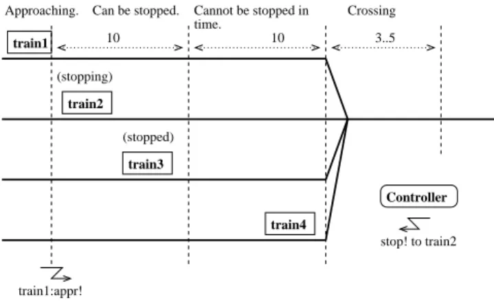
The train gate example is distributed withUppaal. It is a railway control system which controls access to a bridge for several trains. The bridge is a critical shared resource that may be accessed only by one train at a time. The system is defined as a number of trains (assume 4 for this example) and a controller. A train can not be stopped instantly and restarting also takes time. Therefor, there are timing constraints on the trains before entering the bridge. When approaching,
Fig. 12.View of the verification tab for the train gate example.
a train sends a appr! signal. Thereafter, it has 10 time units to receive a stop signal. This allows it to stop safely before the bridge. After these 10 time units, it takes further 10 time units to reach the bridge if the train is not stopped. If a train is stopped, it resumes its course when the controller sends a go! signal to it after a previous train has left the bridge and sent a leave! signal. Figures 13 and 14 show two situations.
4.2 Modelling in Uppaal
The model of the train gate has three templates: Train is the model of a train, shown in Fig. 9.
Gate is the model of the gate controller, shown in Fig. 15.
IntQueue is the model of the queue of the controller, shown in Fig. 16. It is simpler to separate the queue from the controller, which makes it easier to get the model right.
The Template of the Train The template in Fig. 9 has five locations:Safe, Appr, Stop, Start, andCross. The initial location isSafe, which corresponds to a train not approaching yet. The location has no invariant, which means that a train may stay in this location an unlimited amount of time. When a train is approaching, it synchronises with the controller. This is done by the channel synchronisationappr!on the transition to Appr. The controller has a correspondingappr?. The clockxis reset and the parameterised variableeis set
train2
train3
train4
Controller train1
Crossing
10 10 3..5
train1:appr!
stop! to train2 (stopping)
(stopped) Can be stopped.
Approaching. Cannot be stopped in time.
Fig. 13. Train gate example: train4 is about to cross the bridge, train3 is stopped, train2 was ordered to stop and is stopping. Train1 is approaching and sends an appr! signal to the controller that sends back a stop! signal. The different sections have timing constraints (10, 10, between 3 and 5).
to the identity of this train. This variable is used by the queue and the controller to know which train is allowed to continue or which trains must be stopped and later restarted.
The locationAppr has the invariantx ≤20, which has the effect that the location must be left within 20 time units. The two outgoing transitions are guarded by the constraints x≤ 10 andx ≥10, which corresponds to the two sections before the bridge: can be stopped and can not be stopped. At exactly 10, both transitions are enabled, which allows us to take into account any race conditions if there is one. If the train can be stopped (x≤10) then the transition to the locationStop is taken, otherwise the train goes to locationCross. The transition toStopis also guarded by the conditione==idand is synchronised with stop?. When the controller decides to stop a train, it decides which one (setse) and synchronises with stop!.
The locationStophas no invariant: a train may be stopped for an unlimited amount of time. It waits for the synchronisationgo?. The guarde==idensures that the right train is restarted. The model is simplified here compared to the version described in [60], namely the slowdown phase is not modelled explicitly. We can assume that a train may receive a go?synchronisation even when it is not stopped completely, which will give a non-deterministic restarting time.
The location Start has the invariant x ≤ 15 and its outgoing transition has the constraint x≥7. This means that a train is restarted and reaches the crossing section between 7 and 15 time units non-deterministically.
The locationCrossis similar toStartin the sense that it is left between 3 and 5 time units after entering it.
train3
Controller train4 train2
train1
go! to train3 (restarting)
(stopped) (stopping)
train4:leave!
Fig. 14.Now train4 has crossed the bridge and sends a leave! signal. The controller can now let train3 cross the bridge with a go! signal. Train2 is now waiting and train1 is stopping.
The Template of the Gate The gate controller in Fig. 15 synchronises with the queue and the trains. Some of its locations do not have names. Typically, they are committed locations (marked with ac).
The controller starts in the Free location (i.e., the bridge is free), where it tests the queue to see if it is empty or not. If the queue is empty then the controller waits for approaching trains (next location) with the appr? synchro-nisation. When a train is approaching, it is added to the queue with the add! synchronisation. If the queue is not empty, then the first train on the queue (read byhd!) is restarted with thego!synchronisation.
In the Occ location, the controller essentially waits for the running train to leave the bridge (leave?). If other trains are approaching (appr?), they are stopped (stop!) and added to the queue (add!). When a train leaves the bridge, the controller removes it from the queue with therem?synchronisation. The Template of the Queue The queue in Fig. 16 has essentially one location Start where it is waiting for commands from the controller. The Shiftdown location is used to compute a shift of the queue (necessary when the front element is removed). This template uses an array of integers and handles it as a FIFO queue.
4.3 Verification
We check simple reachability, safety, and liveness properties, and for absence of deadlock. The simple reachability properties check if a given location is reach-able:
– E<> Gate.Occ: the gate can receive and store messages from approaching trains in the queue.
– E<> Train1.Cross: train 1 can cross the bridge. We check similar properties for the other trains.
add2 add1
Occ Free
Send
notempty?
empty?
appr?
leave?
stop! go!
hd! appr?
add!
add! rem?
Fig. 15.Gate automaton of the train gate.
– E<> Train1.Cross and Train2.Stop: train 1 can be crossing the bridge while train 2 is waiting to cross. We check for similar properties for the other trains.
– E<> Train1.Cross && Train2.Stop && Train3.Stop && Train4.Stopis similar to the previous property, with all the other trains waiting to cross the bridge. We have similar properties for the other trains.
The following safety properties must hold for all reachable states:
– A[] Train1.Cross+Train2.Cross+Train3.Cross+Train4.Cross<=1. There is not more than one train crossing the bridge at any time. This expression uses the fact thatTrain1.Crossevaluates to true or false, i.e., 1 or 0.
– A[] Queue.list[N-1] == 0: there can never be N elements in the queue, i.e., the array will never overflow. Actually, the model defines N as the num-ber of trains + 1 to check for this property. It is possible to use a queue length matching the number of trains and check for this property instead: A[] (Gate.add1 or Gate.add2) imply Queue.len < N-1where the loca-tionsadd1andadd2are the only locations in the model from whichadd!is possible.
The liveness properties are of the form Train1.Appr --> Train1.Cross: whenever train 1 approaches the bridge, it will eventually cross, and similarly for the other trains. Finally, to check that the system is deadlock-free, we verify the propertyA[] not deadlock.
Suppose that we made a mistake in the queue, namely we wrotee:=list[1] in the templateIntQueueinstead of e:=list[0]when reading the head on the transition synchronised withhd?. We could have been confused when thinking in terms of indexes. It is interesting to note that the properties still hold, except
Start
Shiftdown
i < len list[i]:=list[i+1], i++
len==i list[i] := 0, i := 0 len>=1
rem! len--, i := 0 len==0 empty!
add?
list[len]:=e, len++
hd? e:=list[0] len>0
notempty!
Fig. 16. Queue automaton of the train gate. The template is parameterised with
int[0,n] e.
the liveness ones. The verification gives a counter-example showing what may happen: a train may cross the bridge but the next trains will have to stop. When the queue is shifted the train that starts again is never the first one, thus the train at the head of the queue is stuck and can never cross the bridge.
5
Example 2: Fischer’s Protocol
5.1 Description
Fischer’s protocol is a well-known mutual exclusion protocol designed forn pro-cesses. It is a timed protocol where the concurrent processes check for both a delay and their turn to enter the critical section using a shared variableid. 5.2 Modelling in Uppaal
The automaton of the protocol is given in Fig. 17. Starting from the initial location (marked with a double circle), processes go to a request location,req, if id==0, which checks that it is the turn for no process to enter the critical section. Processes stay non-deterministically between 0 andktime units inreq, and then go to thewaitlocation and setidto their process ID (pid). There it must wait at least k time units,x>k,kbeing a constant (2 here), before entering the critical sectionCSif it is its turn,id==pid. The protocol is based on the fact that after (strict) k time units with iddifferent from 0, all the processes that want to enter the critical section are waiting to enter the critical section as well, but only one has the right ID. Upon exiting the critical section, processes reset idto allow other processes to enterCS. When processes are waiting, they may retry when another process exitsCSby returning toreq.
wait req
x<=k
cs
id== 0 x:= 0
x<=k x:= 0,
id:= pid id== 0 x:= 0
x>k, id==pid id:= 0
Fig. 17.Template of Fischer’s protocol. The parameter of the template is const pid. The template has the local declarationsclock x; const k 2;.
5.3 Verification
The safety property of the protocol is to check for mutual exclusion of the loca-tion CS: A[] P1.cs + P2.cs + P3.cs + P4.cs <= 1. This property uses the trick that these tests evaluate to true or false, i.e., 0 or 1. We check that the system is deadlock-free with the propertyA[] not deadlock.
The liveness properties are of the formP1.req --> P1.waitand similarly for the other processes. They check that whenever a process tries to enter the critical section, it will always eventually enter the waiting location. Intuitively, the reader would also expect the property P1.req --> P1.cs that similarly states that the critical section is eventually reachable. However, this property is violated. The interpretation is that the process is allowed to stay in waitfor ever, thus there is a way to avoid the critical section.
Now, if we try to fix the model and add the invariant x <= 2*k to the wait location, the property P1.req --> P1.csstill does not hold because it is possible to reach a deadlock state whereP1.waitis active, thus there is a path that does not lead to the critical section. The deadlock is as follows: P1.wait with 0≤x≤2 andP4.wait with 2≤x≤4. Delay is forbidden in this state, due to the invariant onP4.waitandP4.waitcan not be left becauseid== 1.
6
Example 3: The Gossiping Girls
6.1 Description
Letngirls have each a private secret they wish to share with each other. Every girl can call another girl and after a conversation, both girls know mutually all their secrets. The problem is to find out how many calls are necessary so that all the girls know all the secrets. A variant of the problem is to add time to conversations and ask how much time is necessary to exchange all the secrets, allowing concurrent calls.
The basic formulation of the problem is not timed and is typically a combi-natorial problem with a string of nbits that may take (at most) 2n values for
every girl. That means we have in total a string ofn2 bits taking 2n2
values (in product with other states of the system).
6.2 Modelling in Uppaal
We face choices regarding the representation of the secrets and where to store them. One way is to use one integer and manually set or reset its bits using arithmetic operations. Although the size of the system is limited by the size of the integers, a quick complexity evaluation shows that the state-space explodes too quicly anyway so this is not really a limitation. Another way is to use an array of booleans. The solution with the integer sounds like hacking and in fact it is so specialized that we will have problem to refine the model later. The model with booleans is certainly more readable, which is desirable for formal verification. The second choice is where to store the messages: in one big shared table locally with every girl process. The referenced models are available at http://www.cs.aau.dk/~adavid/UPPAAL-tutorial/.
Generic Declarations The global declaration contains: const int GIRLS = 4;
typedef int[0,GIRLS-1] girl_t; chan phone[girl_t], reply[girl_t];
This allows us to scale the model easily. Notice that it is possible to declare that arrays of channels are indexed by a given type, which implicitely gives them the right size. This is necessary to use symmetry reduction throughscalarsets later. The girl process is namedGirl and hasgirl t id as parameter. Every girl has a different ID. The systemdeclaration is simply:system Girl;. This makes use of the auto-instantiationfeature of Uppaal. All instances of the template Girl ranging over its parameters are generated. The number of instances is controlled by the constantGIRLS.
Flexible Modelling We declare three local functions to the template Girl. Notice that they have access to the parameterid. These functions are used to initialize the template (start()) with a unique secret and to send and receive secrets to other templates (talk() and listen()). We can change these functions but still keep the same model, which makes the model flexible.
Integers The encoding with integers hasmeta int tmp; added to the global dec-larations and the following to the local declaration of the templateGirl:
girl_t g; int secrets;
void start() { secrets = 1 << id; } void talk() { tmp = secrets; } void listen() { secrets |= tmp; }
Initialization is done by setting bit id to one. The initial committed location ensures all girls are initialized before they start to exchange secrets. Then we have a standard message passing using a shared variable with the receiver merging the secrets sent with her own (logical or). The shared variable is declaredmeta, which means it is a special temporary variable notpart of the state, i.e., never refer to such a variable between two states. We assume that these functions are used with channel synchronization.
Booleans The encoding with booleans has meta bool tmp[girl t]; added to the global declarations and the following to the local declarations of the template Girl:
girl_t g;
bool secrets[girl_t];
void start() { secrets[id] = true; } void talk() { tmp = secrets; }
void listen() { for(i:girl_t) secrets[i] |= tmp[i]; }
In this version we use assignment between arrays fortalk(). The functionlisten() uses an iterator. The automaton for models gossip0.xml (with integers) and gossip1.xml (with booleans) is given in Fig. 18. This first attempt captures the fact that we want the model to be symmetric with respect to sending and receiv-ing and is quite natural with symmetric uses of talk() and listen(). The local variablegrecords which other girl is a given template communicating with. The sender selects its receiver and the receiver its sender.
Reply Listen Ringing
reply[g]? listen() reply[g]!
talk() j : girl_t
phone[j]? listen(), g = j
j : girl_t id != j phone[j]! g = j, talk() start()
Fig. 18.First attempt for modelling the gossiping girls.
Let us first improve the model on three points:
1. The intermediate state Listen should be made committed otherwise all in-terleaving of half-started and complete calls will occur.
2. One select is enough because we are modelling something else here, namely girlid selects a channel jandany other girl that selects the same channel can communicate withid.
3. The local variablegcontributes badly to the state-space when its value is not relevant, i.e., the previous communication does not need to be kept. We can set it in a symmetric manner upon the start and reset it after communication toid.
These are typical “optimizations” of a model: Avoid useless interleavings by using committed locations, make sure you model exactly what you need and not more,
and “active variable reduction”. The updated model (gossip2.xml/integers,gossip3.xml/booleans) is shown in Fig. 19. The template keeps as an invariant that the variable g is
always equal toid whenever it is not sending. In addition, when a channeljis selected, then it corresponds to exactly girlj. Only one committed location is enough but it is a good practice to mark them both. It is more explicit when we read the model. Since the model performs better, we can now check with 5 girls instead of 4 within roughly the same time, which is a very good improvement considering the exponential complexity of the model.
Reply Listen Ringing
reply[g]? listen(), g = id reply[id]!
talk() phone[id]? listen()
j : girl_t id != j phone[j]! g = j, talk() start(), g = id
Fig. 19.Improved model of the gossiping girls.
Optimizing Further We can abstract which communication line is used by declar-ing only one channelchan call. Since the semantics says that any pair of enabled edges(call!,call?) can be taken, we do not need to make an extra select. In addi-tion, processes cannot synchronize with themselves so we do not need this check either. The downside is that we lose the information on the receiver from the sender point of view. We do not need this in our case. We can get rid of the local variablegas well. We could use the sequencetalk()-listen()-talk()-listen() with the old functions but we can simplify these by merging the middlelisten()-talk() into one and simplifyinglisten() to a simple assignment since we know that the message already contains the secrets sent. The global declaration is updated with onlychan call; for the channel. The updated automaton is depicted in Fig. 20.
Theintegerversion of the model (gossip4.xml) has the following local func-tions:
Listen Ringing
listen() call?
exchange()
call! talk() start()
Fig. 20.Optimized model of the gossiping girls.
int secrets;
void start() { secrets = 1 << id; } void talk() { tmp = secrets; }
void exchange() { secrets = (tmp |= secrets); } void listen() { secrets = tmp; }
Theboolean version of the model (gossip5.xml) is changed to: bool secrets[girl_t];
void start() { secrets[id] = true; } void talk() { tmp = secrets; }
void exchange() { for(i:girl_t) tmp[i] |= secrets[i]; secrets = tmp; }
void listen() { secrets = tmp; }
The exchange function could have been written as void exchange() {
for(i:girl_t) secrets[i] = (tmp[i] |= secrets[i]); }
which is almost the same. The difference is that the number of interpreted in-structions is lower in the first case. A step further would be to inline these functions on the edges in the model but then we would lose readability to gain less than 5% in speed. It is possible to further optimize the model by having one parameterized shared table and avoid message passing all-together. We leave this as an exercise for the reader but we notice that this change destroys the nice design with the local secrets to each process.
6.3 Verification
We check the property that all girls know all secrets. For the integer version of the model, the property is:
E<> forall(i:girl_t) forall(j:girl_t) (Girl(i).secrets & (1 << j)) We can write a shorter but less obvious equivalent formula that takes advantage of the fact that 2GIRLS−1 generates a bit mask with the first GIRLS bits set to one:
E<> forall(i:girl_t) Girl(i).secrets == ((1 << GIRLS)-1) The formula for the boolean version is:
E<> forall(i:girl_t) forall(j:girl_t) Girl(i).secrets[j]
The formulas use the “for-all” construct, which gives compact formulas that automatically scale with the number of girls in the model. The version with the integers checks with a bit mask that the bits are set.
Table 1 shows the resource consumption for the different models with different number of girls. Experiments are run on an AMD Opteron 2.2GHz withUppaal rev. 2842. The results show how important it is to be careful with the model and
Girls 4 5 6
gossip0 0.6s/24M 498s/3071M -gossip1 1.0s/24M 809s/3153M -gossip2 0.1s/1.3M 0.3s/22M 71s/591M gossip3 0.1s/1.3M 0.5s/22M 106s/607M gossip4 0.1s/1.3M 0.2s/22M 37s/364M gossip5 0.1s/1.3M 0.3s/22M 63s/381M
Table 1.Resource consumption for the different models with different number of girls. Results are in seconds/Mbytes.
to optimize the model to reduce the state-space whenever possible. We notice that we do not even have time in this model. The model with integers is faster due to its simplicity but consumes marginally less memory.
6.4 Improved Verification
Uppaalfeatures two major techniques to improve verification. These techniques concern directly verification and are orthogonal to model optimization. The first is symmetry reduction. Since we designed our model to be symmetric from the start, taking advantage of this feature is done by using ascalar setfor the type girl t. The second feature is the generalized sweep-line method. We need to define a progress measure to help the search. Furthermore, only the model with booleans is eligible for symmetry reduction since we cannot access individual bits in an integers in a symmetric manner (using scalars).
Symmetry Reduction The only change required is for the definition of the type girl t. We use a scalar set for the new model (gossip6.xml):
Sweep-line We need to define a progress measure that is cheap to compute and relevant to help the search. It is important that it is cheap to compute since it will be evaluated for every state. To do so, we addint m; to the global declarations, we add the progress measure definitionafterthe system declaration:
progress { m; }
Finally, we compute min the exchange function as follows: void exchange() {
m = 0;
for(i:girl_t) {
m += tmp[i] ^ secrets[i]; tmp[i] |= secrets[i]; }
}
This measures counts the number of new messages exchanged per communica-tion.
Girls 4 5 6 7
gossip6 0.1s/1.3M 0.1s/1.3M 3.4s/29M 399s/1115M gossip7 0.1s/1.3M 0.1s/1.3M 0.3s/21M 29s/108M
Table 2. Resource consumption using symmetry reduction (gossip6) combined with the sweep-line method (gossip7).
Table 2 show that these features give gains with another order of magnitude both in speed and memory. The model still explodes exponentially but we cannot avoid it given its nature.
7
Modelling Patterns
In this section we present a number of useful modelling patterns for Uppaal. A modelling pattern is a form of designing a model with a clearly stated intent, motivation and structure. We observe that most of ourUppaalmodels use one or more of the following patterns and we propose that these patterns are imitated when designing new models.
7.1 Variable Reduction Intent
To reduce the size of the state space by explicitly resetting variables when they are not used, thus speeding up the verification.
Motivation
Although variables are persistent, it is sometimes clear from the way a model behaves, that the value of a variable does not matter in certain states, i.e., it is clear that two states that only differ in the values of such variables are in fact bisimilar. Resetting these variables to a known value will make these two states identical, thus reducing the state space.
Structure
The pattern is most easily applied to local variables. Basically, a variable v is called inactive in a locationl, if along all paths starting from l,v will be reset before it will be used. If a variablev is inactive in locationv, one should resetv
to the initial value on all incoming edges ofl.
The exception to this rule is whenv is inactive in all source locations of the incoming edges tol. In this case,v has already been reset, and there is no need to reset it again. The pattern is also applicable to shared variables, although it can be harder to recognise the locations in which the variable will be inactive.
For clocks, Uppaal automatically performs the analysis described above. This process is called active clock reduction. In some situations this analysis may fail, since Uppaal does not take the values of non-clock variables into account when analysing the activeness. In those situations, it might speed up the verification, if the clocks are reset to zero when it becomes inactive. A similar problem arises if you use arrays of clocks and use integer variables to index into those arrays. Then Uppaal will only be able to make a coarse approximation of when clocks in the array will be tested and reset, often causing the complete array to be marked active at all times. Manually resetting the clocksmight speed up verification.
Sample
The queue of the train gate example presented earlier in this tutorial uses the active variable pattern twice, see Fig. 21: When an element is removed, all the remaining elements of the list are shifted by one position. At the end of the loop in the Shiftdownlocation, the counter variableiis reset to 0, since its value is no longer of importance. Also the freed up element list[i]in the list is reset to zero, since its value will never be used again. For this example, the speedup in verification gained by using this pattern is approximately a factor of 5. Known Uses
The pattern is used in most models of some complexity. 7.2 Synchronous Value Passing
Intent
To synchronously pass data between processes. Motivation
Start
Shiftdown
i < len list[i]:=list[i+1], i++
len==i list[i] := 0, i := 0 len>=1
rem! len--, i := 0 len==0 empty!
add?
list[len]:=e, len++
hd? e:=list[0] len>0
notempty!
Fig. 21.The model of the queue in the train gate example uses active variable reduction twice. Both cases are on the edge fromShiftdowntoStart: The freed element in the queue is reset to the initial value and so is the counter variablei.
as processes. Neighbouring nodes must communicate to exchange, e.g., routing information. Assuming that the communication delay is insignificant, the hand-shake can be modelled as synchronisation via channels, but any data exchange must be modelled by other means.
The general idea is that a sender and a receiver synchronise over shared binary channels and exchange data via shared variables. SinceUppaalevaluates the assignment of the sending synchronisation first, the sender can assign a value to the shared variable which the receiver can then access directly.
Structure
There are four variations of the value passing pattern, see Fig. 22. They differ in whether data is passedone-way ortwo-way and whether the synchronisation is unconditional or conditional. In one-way value passing a value is transfered from one process to another, whereas two-way value passing transfers a value in each direction. In unconditional value passing, the receiver does not block the communication, whereas conditional value passing allows the receiver to reject the synchronisation based on the data that was passed.
In all four cases, the data is passed via the globally declared shared variable varand synchronisation is achieved via the global channelscandd. Each process has local variablesinand out. Although communication via channels is always synchronous, we refer to ac!as a send-action andc?as a receive-action. Notice that the variable reduction pattern is used to reset the shared variable when it is no longer needed. Alternatively, the shared variable can be declaredmeta, in which case the reset is not necessary since the variable is not part of the state.
In one-way value passing only a single channelcand a shared variablevar is required. The sender writes the data to the shared variable and performs a
Unconditional Conditional O n e-w ay c! var := out
‚ ‚ ‚ ‚ ‚ c? in := var, var := 0
c! var := out
‚ ‚ ‚ ‚ ‚ cond(in) c? in := var, var := 0
A sy m m et ri c tw o -w
ay c!var := out
d? in := var, var :=0 ‚ ‚ ‚ ‚ ‚ c? in := var
d! var := out
cond1(var) c! var := out
d? in := var, var :=0 ‚ ‚ ‚ ‚ ‚ cond2(in) c? in := var, var := out
d!
Fig. 22.The are essentially four combinations of conditional, unconditional, one-way and two-way synchronous value passing.
send-action. The receiver performs the co-action, thereby synchronising with the sender. Since the update on the edge with send-action is always evaluated before the update of the edge with the receive-action, the receiver can access the data written by the sender in the same transition. In the conditional case, the receiver can block the synchronisation according to some predicate cond(in)involving the value passed by the sender. The intuitive placement of this predicate is on the guard of the receiving edge. Unfortunately, this will not work as expected, since the guards of the edges are evaluated before the updates are executed, i.e., before the receiver has access to the value. The solution is to place the predicate on the invariant of the target location.
Two-way value passing can be modelled with two one-way value passing pat-tern with intermediate committed locations. The committed locations enforce that the synchronisation is atomic. Notice the use of two channels: Although not strictly necessary in the two-process case, the two channel encoding scales to the case with many processes that non-deterministically choose to synchro-nise. In the conditional case each process has a predicate involving the value passed by the other process. The predicates are placed on the invariants of the committed locations and therefore assignment to the shared variable in the sec-ond process must be moved to the first edge. It might be tempting to encoding conditional two-way value passing directly with two one-way conditional value passing pattern, i.e., to place the predicate of the first process on the third location. Unfortunately, this will introduce spurious deadlocks into the model.
If the above asymmetric encoding of two-way value passing is undesirable, the symmetric encoding in Fig. 23 can be used instead. Basically, a process can non-deterministically choose to act as either the sender or the receiver. Like before,
committed locations guarantee atomicity. If the synchronisation is conditional, the predicates are placed on the committed locations to avoid deadlocks. Notice that the symmetric encoding is more expensive: Even though the two paths lead to the same result, two extra successors will be generated.
cond(var) cond(in)
c! var := out
in := var, var := 0 d?
c? in := var, var := out
d!
Fig. 23.In contrast to the two-way encoding shown in Fig 22, this encoding is sym-metric in the sense that both automata use the exact same encoding. The symmetry comes at the cost of a slightly larger state space.
Sample
The train gate example of this tutorial uses synchronous one-way unconditional value passing between the trains and the gate, and between the gate and the queue. In fact, the value passing actually happens between the trains and the queue and the gate only act as a mediator to decouple the trains from the queue. Known Uses
Lamport’s Distributed Leader Election Protocol. Nodes in this leader election protocol broadcast topology information to surrounding nodes. The communi-cation is not instantaneous, so an intermediate process is used to model the message. The nodes and the message exchange data via synchronous one-way unconditional value passing.
Lynch’s Distributed Clock Synchronisation Protocol. This distributed protocol synchronises drifting clocks of nodes in a network. There is a fair amount of non-determinism on when exactly the clocks are synchronised, since the proto-col only required this to happen within some time window. When two nodes synchronise non-deterministically, both need to know the other nodes identity. As an extra constraint, the synchronisation should only happen if it has not happened before in the current cycle. Here the asymmetric two-way conditional value passing pattern is used. The asymmetric pattern suffices since each node has been split into two processes, one of them being dedicated to synchronising with the neighbours.
7.3 Synchronous Value Passing (bis) Intent
To synchronously pass integers with a small range between processes. Motivation
Similarly to the previous value passing pattern, it is useful to send values between processes. However, this pattern is specialized to integers with small ranges, which gives us the benefit to avoid using a shared variable for the communica-tion.
Structure
The idea is to use arrays of channels to pass specific integers. The pattern is given for the general case of passing an integer value betweenMIN andMAX. Declare the arraychan send[MAX-MIN+1] withMAX and MIN being either constants or the actual value of the desired range. Figure 7.3 shows the pattern. As an example the sender is sending the values 2, 3, or a randomly chosen value. The receiver is using the select feature of Uppaal3.6 to find the right value. Notice that this is expensive for the model-checker if the range is large and will degrade performance. Two-way value passing can be modeled similarly to the previous pattern with the shared variable removed. Conditional value passing works for one-way only.
sent send[3-MIN]!
send[2-MIN]!
random:int[MIN,MAX] send[random-MIN]!
‚ ‚ ‚ ‚ ‚
received i:int[MIN,MAX] send[i-MIN]? value=i
(a) Sender. (b) Receiver. Fig. 24.Value passing using an array of channels.
7.4 Multicast Intent
To encode multicast to at leastN receivers (or similarly exactlyN). Motivation
Uppaal provides pair-wise synchronisation via regular channels (chan) and broadcast synchronisation via broadcast channels (broadcast chan). In some models it is useful to ensure there are at leastN receivers available and have the multicast behaviour, typically for communication protocols.
Structure
location where it is possible to receive and decrement this variable on the edges that leave this location. In addition, add the constraint in the sender process on the required number of receiver (e.g. ready >=N). Figure 7.4 illustrates the patter.
sentN waitN
ready >= 3 multisend!
‚ ‚ ‚ ‚ ‚
received waiting doSomething
multisend? ready--ready++
(a) Sender. (b) Receiver.
Fig. 25.Multicast from one sender to at leastN receivers (3 in this example).
7.5 Atomicity Intent
To reduce the size of the state space by reducing interleaving using committed locations, thus speeding up the verification.
Motivation
Uppaal uses an asynchronous execution model, i.e., edges from different au-tomata can interleave, andUppaalwill explore all possible interleavings. Partial order reduction is an automatic technique for eliminating unnecessary interleav-ings, butUppaaldoes not support partial order reduction. In many situations, unnecessary interleavings can be identified and eliminated by making part of the model execute in atomic steps.
Structure
Committed locations are the key to achieving atomicity. When any of the pro-cesses is in a committed location, then time cannot pass and at least one of these processes must take part in the next transition. Notice that this does not rule out interleaving when several processes are in a committed location. On the other hand, if only one process is in a committed location, then that process must take part in the next transition. Therefore, several edges can be executed atomically by marking intermediate locations as committed and avoiding syn-chronisations with other processes in the part that must be executed atomically, thus guaranteeing that the process is the only one in a committed location. Sample
Start
Shiftdown
i < len list[i]:=list[i+1], i++
len==i list[i] := 0, i := 0 len>=1
rem! len--, i := 0 len==0 empty!
add?
list[len]:=e, len++
hd? e:=list[0] len>0
notempty!
Fig. 26. When removing the front element from the queue, all other elements must be shifted down. This is done in the loop in theShiftdown location. To avoid unnec-essary interleavings, the location is marked committed. Notice that the edge entering
Shiftdown synchronises over theremchannel. It is important that target locations of edges synchronising overremin other processes are not marked committed.
Known Uses
Encoding of control structureA very common use is when encoding control struc-tures (like the encoding of a for-loop used in theIntQueueprocess of the train-gate example): In these cases the interleaving semantics is often undesirable. Multi-castingAnother common use is for complex synchronisation patterns. The standard synchronisation mechanism inUppaalonly supports binary or broad-cast synchronisation, but by using committed locations it is possible to atomi-cally synchronise with several processes. One example of this is in the train-gate example: Here theGateprocess acts as a mediator between the trains and the queue, first synchronising with one and then the other – using an intermediate committed location to ensure atomicity.
7.6 Urgent Edges Intent
To guarantee that an edge is taken without delay as soon as it becomes enabled. Motivation
Uppaal provides urgent locations as a means of saying that a location must be left without delay. Uppaal provides urgent channels as a means of saying that a synchronisation must be executed as soon as the guards of the edges involved are enabled. There is no way of directly expressing that an edge without synchronisation should be taken without delay. This pattern provides a way of encoding this behaviour.
Structure
The encoding of urgent edges introduces an extra process with a single location and a self loop (see Fig. 27 left). The self loop synchronises on theurgentchannel go. An edge can now be made urgent by performing the complimentary action (see Fig. 27 right). The edge can have discrete guards and arbitrary updates, but no guards over clocks.
go!
‚ ‚ ‚ ‚ ‚
go?
Fig. 27.Encoding of urgent edges. Thegochannel is declared urgent.
Sample
This pattern is used in a model of a box sorting plant (seehttp://www.cs.auc. dk/∼behrmann/esv03/exercises/index.html#sorter): Boxes are moved on a belt, registered at a sensor station and then sorted by a sorting station (a piston that can kick some of the boxes of the belt). Since it takes some time to move the boxes from the sensor station to the sorting station, a timer process is used to delay the sorting action. Figure 28 shows the timer (this is obviously not the only encoding of a timer – this particular encoding happens to match the one used in the control program of the plant). The timer is activated by setting a shared variableactive to true. The timer should then move urgently from the passive location to the waitlocation. This is achieved by synchronising over the urgent channelgo.
wait x<=ctime
passive
x==ctime eject! active:=false
active==true go?