AbstractThis paper describes the development and
application of a transfer hydrograph approach to flood forecasting on the Cimanuk River at the city of Jatigede in West Java, Indonesia. The Transfer Hydrograph (TH) is a transfer function that transforms total rainfall into a flood hydrograph at the basin outlet. As opposed to the conven-tional unit hydrograph approach which uses effective rain-fall and direct runoff, the transfer hydrograph uses the to-tal rainfall and the direct runoff at the basin outlet. The Ci-manuk river basin (drainage area : 1,442 km2) has four sub
basins. It was found to be necessary to further extend the application of the transfer hydrograph concept to include all channel routing effects. This because the rainfall at each subbasin was found to be quite independent of the rainfall at other sub basins, and run off data were only available at the basin outlet at Jatigede. Using the available data, trans-fer hydrograph were derived for each sub basin and later combined to give the runoff hydrograph at Jatigede. The approach was tested against recorded rainfall-run off data at Jatigede and was found to give very reasonable results. For flows above 300 m3/second, the maximum error of
pre-diction was less than 12 %.
Keywordstransfer hydrograph, unit hydrograph, rain-fall
I. INTRODUCTION
he Cimanuk river is located in West Java, Indone-sia. Prior to 1980, overtopping of the banks of this river caused severe flooding to down stream areas of the City of Jatigede about 4 to 5 times a year. The flooded areas included 55,000 hectares of rice fields, about 100 villages, and the cities of Indramayu and Kadipaten.
In 1977 the Government of Indonesia proposed a two stage plan to protect the areas prone to flooding. The first step was to protect the city of Indramayu, the 50,000 hectares of rice field, and most of the villages, by con-structing about 200 km of dyke along the river. The dikes were designed based on flood discharges with return periods ranging from 10 to 25 years, depending on the location. However, there are presently about 5,000 hectares of rice fields and many villages that are not protected from flooding. These areas are now being used as detention basins to attenuate the flood peaks to reduce the effects of flooding on downstream areas. The second step in the government plan was to protect all the areas prone to flooding by meant of a flood control dam at Jatigede. This dam was scheduled to be built in 1985. However because of funding problems, the construction of this dam has been postponed until 2010 and will be fi-nished completely in 2020.
At present there are two alternatives available to mini-mize the impacts of flooding on these unprotected areas.
1Saihul Anwar, is Functional Goverment, Ministry of Public Work,
Bina Marga Bulding 8th floor, Jl. Pattimura No.20 Kebayoran Baru,
Jakarta Selatan, 12110, Indonesia. E-mail: [email protected].
6
The first alternative is to build dikes along the present detention basins and to raise the height of the dikes downstream. This alternative is very expensive and almost impossible to be realized at present economic situation. The second alternative is to establish a flood forecasting and warning system for the flood prone areas. The later alternative although will not protect against property damage but at least will prevent loss of life and is also considered as the most effective alterna-tive at present. This paper describes one kind of such flood forecasting method, a method based on a “Transfer Hydrograph” approach.
II. THE STUDY AREA
The Cimanuk river basin is located in the tropical zone just below the equator. Its temperature and humidity are relatively constant throughout the year. The average monthly air temperature at Jatigede ranges from 260 to
280Celsius. The average annual humidity is about 84 %,
and the average wind speed is about 1.85 m/s.
Rainfall event are localized and generally occur in the afternoon lasting between a few minutes to several hours. Most of the heavy rainfall occurs during the wet monsoon season between Novembers to May. The average annual rainfall in the Cimanuk basin varies from 2000 mm at the lower elevation to 4000 mm in the most upstream portions of the basin. The average annual run-off the Cimanuk River at Jatigede is about 470 m3/s and
the maximum recorded runoff was 1470 m3/s, which
occurred in 1978.
The total drainage area of the Cimanuk River upstream of Jatigede is about 1,442 km2. The main stream length
is about 85 km with the channel width ranging from 20 m at Cikajang Station to 50 m at Malangbong station. The difference in elevation of the river over the 85 km length is about 1000 m. The land used in basin is mainly rice field and fish ponds. These rice field and fish ponds provide large areas and have a significant influence on the hydrology of the basin. The soil is of volcanic origin and is extremely fertile.
III. METHODOLOGY
Flood forecasting systems have been widely used to predict the magnitude of discharge so as to mitigate the loss of life and property caused by flooding. Many mo-dels have been developed for flood forecasting purposes. Using a model, the flood discharge at a certain point in the river can be estimated from the rainfall data that are inputted into the model. The method for estimating the magnitude of discharge is based on the availability of data and on whether the characteristics of the basin are well understood.
Saihul Anwar16
Flood Forecasting using a Transfer Hydrograph
Approach
Two types of basins can be distinguished depending on the availability of data. The first type is a basin where the physical characteristics of the basin is well documented. The second type is a basin where the physical cha-racteristics of the basin have not been well documented.
Many models are developed based on the assumption that almost all the physical phenomenon of nature such as evaporation, infiltration, storage, overland flows, and channel flows are known and can be taken into account in transforming rainfall into runoff. These models can be successfully used if the physical processes in trans-forming rainfall into run off are well understood. Some examples of this type of flood forecasting models are HEC-1 (1973), HYMO (1972), and the TR-20 (1973).
There are several limitations of computer simulation models, such as the HEC-1, HYMO, and the TR-20 as described by Victor Miguel Ponce (1989). These include: a. misinterpretation in determining the physical
characteristics of the basin,
b. the model can only be used for a specific design, but it can not determine alternative design, and
c. a weak input data set can still produce an output. When the physical characteristic of the basin are not well documented then the black box models are used in transforming rainfall data into runoff, regardless of the physical process of the transformation. Examples of the black box models include Multiple Regression Models and those based on the Unit Hydrograph approach.
An application of multiple regression in flood fore-casting for example was discussed by Liang (1988). He developed a model for flood forecasting in the Hankou Basin in China using a multiple input, single output, linear, and time invariant regression model. The flow drograph at Hankou was estimated based on the flow hy-drographs at the outlet of three tributaries; Hanjiang Ri-ver, Changjiang RiRi-ver, Qingjiang RiRi-ver, and the spillway outlet of Dongting lake.
The concept of a unit hydrograph (UH) was originally proposed by Sherman (1932). There are two types of unit hydrograph. The first uses the recorded rainfall-runoff data in its derivation. The second type, which is known as a synthetic unit hydrograph, is empirical derived. For example, Snyder (1938) developed a synthetic unit hy-drograph based on the physical geometry of the area. However, it is always preferable to avoid relying on syn-thetic UH’s if non synsyn-thetic UH’s can be developed. Laurenson and O’Donnel (1969) examined four methods of deriving unit hydrograph using rainfall-runoff data. The four methods were: Harmonic analysis, Meixner polynomials, Least squares, and a method due to Nash. A comparison of the results indicated that no one method was better than any other methods, from general point of view. Dooge and Garvey (1970) studied the same four methods for the unit hydrograph derivation and found that the least squares was the best method for good data, but the worst method for bad data and that Meixner poly-nomials was the worst for erroneous data.
Dooge (1979) discussed four categorious of methods, which can be used to derived unit hydrograph.
The four categorious were Direct Matrix Inversion, Optimization, Transform System Methods, and
Identifi-cation Using Conceptual Models. The first category of methods was Matrix Inversion and this category con-sisted of forward substitution, backward substitution, and the Collins method of matrix inversion. The second cate-gory was optimization methods and these consisted of least squares, regularization and quadratic programming methods. The third category, known as Transform Sys-tems, included : Z-Transform, Harmonic Analysis, and Meixner Analysis. The fourth category was identification of unit hydrograph based on Conceptual Models. These consisted of single reservoir, triangle, two equal voirs, routed triangle, routed rectangle, and n equal reser-voirs method. Based on detailed comparison of the va-rious methods Dooge recommended three methods: Har-monic Analysis, Meixner Analysis, and the conceptual Model using n equal reservoirs.
Singh (1976) compared the use of Linear Programming and Least Squares Methods in the derivation of unit hy-drograph. The Linear Programming method minimized the sum of absolute errors and the Least Squares Method minimized sum of the squares of errors. The Linear Pro-gramming Techniques constrained the ordinates of the unit hydrograph to be positive. The results of the study showed that two of the results of the test were the same, while two others showed some deviation in the unit hy-drographs.
Singh, Baniukiewicz, and Ram (1982) (quoted in Singh, 1988, pp. 181) studied nine procedures to derive the unit hydrograph. The nine procedures were: matrix Methods (MT), Forward Substitution (FS), Successive Over-Relaxation (SOR), Least Squares (LS), Harmonic Analysis (HA), Laguerre Polynomials (LP), Meixner Polynomial (MP), Time Series Method (TS), and Linear Programming Method (LPM). They concluded that LP, HA and LS were the best methods to derive unit hydro-graph.
Mawdsley and Tagg (1981) discussed a house holder Transformation Technique to solve the ill-conditioned sets of equations. Several events were analyzed simul-taneously to minimize the difference between the ob-served and computed ordinates of the unit hydrographs. It was shown that better unit hydrographs can be ob-tained using the House holder Transformation in analyzing several events simultaneously. They concluded that the more the number of events analyzed the better the results will be.
Bruen and Dooge (1984) discussed an efficient and robust method for estimating unit hydrograph ordinates. They concluded that the Smoothed Least Squares is an effective method to overcome the instability of unit hy-drograph due to numerical ill-conditioning.
Wang (1986) discussed four methods of estimating the parameters of discrete linear input-output models. The four methods used for estimating of parameters were: Li-niear Programming, Quadratic Programming, Least Squares Estimates, and Correlation Function Estimates. He found that the Quadratic Programming and the Least Squares Estimates gave the best fit.
Smooth-ed Least Squares Method in the derivation of unit hydro-graph. They concluded that the Forward Substitution Method, the amplification of error was greater when the intensity of effective rainfall increased during a storm.
From the above foregoing it can be seen that different conclusions have been reached by various hydrologist concerning the best method of deriving unit hydrograph. However, many researchers recommended the use of the Least Squares Methods to derive the unit hydrographs from rainfall-runoff data.
The techniques considered in this research were re-stricted to black-box approaches because of the lack of hydrology data for the four sub basins. Two techniques were used in developing the flood forecasting model for the Cimanuk River Basins. One method was based on multiple regression, and another method was based on the concept of the Transfer Hydrograph, which was a modification of the classical unit hydrograph because of the un availability of runoff data at each the three sub basins outlet; the Cikajang, the Dayeuh Manggung, and the Wanaraja.
Very few drainage basins in Indonesia have been studied in detail in terms of their drainage characteristics, land used, etc. Rainfall – run off modeling has therefore been mainly restricted to black box type models re-quiring only rainfall and run off data. The Cimanuk River basin is no exception. Based on the topography of the area, the Cimanuk Basin can be divided into four sub basins: Cikajang, Dayeuh Manggung, Wanaraja, and Malangbong (see Fig. 1). Hourly rainfall data were available at each of the four sub basins. However run off data were available at the basin outlet Jatigede. Each sub basin rainfall event had to be taken into account separa-tely.
The technique that was used to develop the flood forecasting model for the Cimanuk River was based on the concept of a transfer hydrograph (TH). The TH is a modification of the classical unit hydrograph which take into account the unavailability of the runoff data at the outlet of each of the sub basins. The TH for a given sub basin is the hydrograph at the basin outlet (Jatigede) caused by 1 unit of total rainfall occurring over that sub basin, as illustrated in Fig. 1. Rainfall losses and routing effects area both taken into account in the transfer hydrograph.
The difference between the classical unit hydrograph (UH) approach and the transfer hydrograph (TH) ap-proach as applied in this study are:
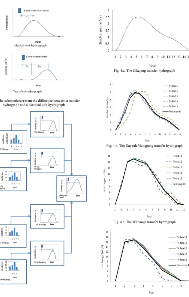
a. The UH is derived based on the effective rainfall, whereas the TH is derived based on the total rainfall, see Fig. 2,
b. The direct run off depth based on the UH is equal to 1 unit of depth, whereas the runoff depth based on the TH will be less than 1 unit of depth because of the hydrologic abstractions, and
c. In the UH the outlet of each sub basin is located at the end of each sub basin. With the TH the outlet for each sub basin is located at the basin (not sub basin) outlet. Except for the above differences all other assumptions such as linearity, are employed in the transfer hydrograph approach.
A. Data Requirement and Assumption for Development of The Transfer Hydrograph
Rainfall–runoff data used in developing and validating each of the transfer hydrographs were of four types. Type A event were those where rainfall occurred only in one sub basin. Type B events were those where rainfall occurred in two sub basins. Type C event were those where rainfall occurred in any three sub basins, and type D event were those where rainfall occurred in all four sub basins. The ideal situation would be to use only type A rainfall–runoff data to develop the transfer hidrograph for all the sub basins. However, since type A event were only available for the Cikajang sub basin, only the Cija-kang sub basin TH could be develop using type A events. For all other sub basins, the rainfall run off data could only be used to derive TH’s by applying the prin-ciple of superposition to maximize the advantage. How these various types of events were used to derive the transfer hydrograph will be illustrated later.
The following assumptions were made in developing the transfer hydrograph.
1. The rainfall was considered to be uniformly distri-buted over a given sub basin.
2. The flow from a sub basin was assumed to have no effect on the flow coming from the other sub basins. 3. The base flow was determined using the straight line
method.
4. The conceptual rainfall – runoff model depicted in Fig. 3 was applied for flood forecasting, in this stu-dy. All four sub basins were considered to have their outlet at the same point, Jatigede (where the dis-charged was observed). This meant that the derived TH’s would have included the effect of channel routing.
B. Procedure
The one hour transfer hydrograph were derived using the “least squares” method (Singh, 1988). The general equation to derive a transfer hydrograph is given by:
[Q] = [I] x [U] (1)
where [Q] is the vector of runoff ordinates in m3/second,
[I] is a special banded matrix of rainfall in mm, where the bandwidth of the [I] matrix is equal to the duration of the rainfall (1), and [U] is the vector of transfer hydro-graph ordinates. The ordinates of the transfer hydrohydro-graph [U] were then computed using the least squares equation by:
[U] = [ITI]-1x [IT] x [Q] (2)
where [IT] is the transpose of matrix [I], and [ITI]-1is the
inverse matrix of [ITI].
The relationship among the rainfall duration (i), the number of transfer hydrograph ordinates (j), and the number of hydrograph ordinates (n) is given by:
n = j+i-1 (3)
The one hour transfer hydrograph for each sub basin was derived according to the type of rainfall event avail-able. For example, for the Cikajang sub basin, type A events were used. The TH was derived using directly, that is [2]:
[Uc]= [IcTIc]1 x [IcT] x [Qc] (4)
For the Wanaraja sub basin, type B event were used because there were no type A events available at this sub basin. The one hour TH for this sub basin had to be ob-tained using the principle of superposition that is:
[Qw]= [QT]-[Ic] x [Uc]tc (5)
and
[Uw]= [IwTIw]1x [IwT] x [Qw] (6)
Where the subscript w refers to the Wanaraja sub basin and tc is travel time of the flow from the Cikajang sub
basin which had to be added to the Cikajang convoluted hydrograph. Other terms are as previously defined.
The transfer hydrograph for Dayeuh Manggung and Malangbong sub basins were computed similarly except that type C event was used. Where there were more than one transfer hydrograph available at each sub basin, the average was taken to be the representative transfer hy-drograph for that sub basin. Type D was used to validate the transfer hydrograph. The validation of transfer hydro-graph was carried out by comparing the convoluted hy-drograph at Jatigede with the observed peak flows and ti-me lags.
IV. RESULT
From the procedure described above, two sets of result were obtained. The first set was the ordinates of the four transfer hydrograph, while the second set was the lag time for each of the transfer hydrographs. The time lag was defined as difference between the time at the begin-ning of rainfall and the peak flow as shown in Fig. 2.
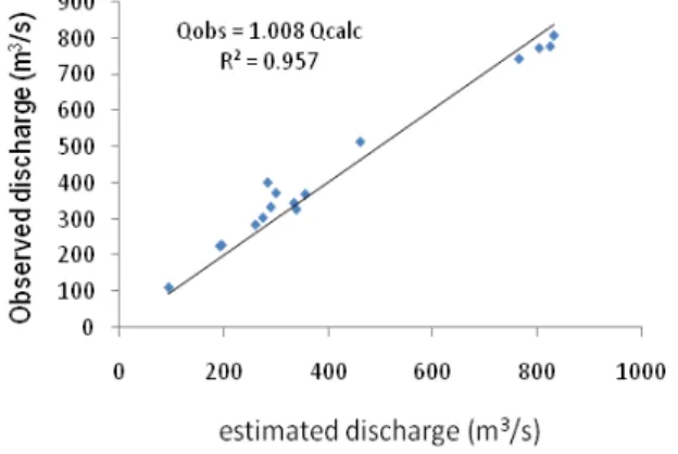
The derived transfer hydrograph for the Cikajang, Dayeuhmanggung Wanaraja, and Malangbong sub ba-sins are shown in Fig. 4a, 4b, 4c, and 4d or Table 3, 4, 5, and 6. The approximate run off coefficients were 0.42, 0.44, 0.51, and 0.56 respectively. The delay time, time to peak, and time lag obtained for each transfer hydrograph are shown in Table 1. Comparing of the observed, the computed peak flows, and the time lags.
Using the time lags and transfer hydrograph derived for each sub basin, sixteen type D events were used to com-pare the accuracy of the predicted peak flows. Table 2 and Fig. 5 show the comparison between the computed and the observed peak flows. It can be seen that for peak flows greater than 300 m3/s, the maximum percentage
error of prediction was less than 12 %. For the time lags, the computed values were practically identical to that of the observed values.
V. CONCLUSION
A transfer hydrograph approach to forecast floods on the Cimanuk River was presented. The approach is a modification of the classical unit hydrograph to deal with the unavailable of sub basin rainfall–runoff data and lo-calized nature of the rainfall. It was shown that for peak flows greater than 300 m3/s, the error prediction was less
than 12 %, which seems reasonable for the simplifying assumption made in the derivation of the transfer hydro-graph.
The transfer hydrograph concept gave better prediction as the magnitude of a discharge increase. For this reason, the Transfer Hydrograph was not suggested to predict the
discharge, where the magnitude of the discharge is less than 600 m3/s. However, for the flood forecasting
purpose, the magnitude of a discharge was considered to be a flood discharge when the magnitude of the dis-charge exceeds 600 m3/s.
REFERENCES
[1] P.B. Bruen and W.C. Huber, 1988, Hydrology and Floodplain Analysis, Addison-Wesley Publishing Company, New York. 650 p. Bruen, P.B., and Dooge J.C.I. “An efficient and robust method for estimating unit hydrograph ordinates”, Journal of Hydrology, Vol. 70, pp.1-24.
[2] M. Dooge and Bruen, 1989, “Unit hydrograph stability and linear Algebra”, Journal. Hydrology, Vol. 111, pp. 377-390.
[3] J.C.I. Dooge and B.J. Garvey, 1970, “Discussion of data error effects in unit hydrograph derivation by E.M. Laurenson and T.O’Donnell“, Journal of the Hydraulics Division, Proceeding of the American Society of civil Engineers, Vol. 96, pp. 1888-1894. [4] J.C.I. Dooge, 1979, “Deterministic input-output models”, The
Mathematics of Hydrology and Water Resources, ed Lloyd, E.H., O’Donnell, T., and Wilkinson, J.C., Academic Press Inc., New York, pp.1-35.
[5] M. Dooge and Bruen, 1989, “Unit hydrograph stability and linear Algebra”, Journal of Hydrology,Vol.111, pp.377-390.
[6] P.J. Huber, 1973, “Robust regression: Asymptotics, Conjectures, and Monte Carlo“, Analysis of Statistics I, pp. 799-821.
[7] E.M. Laurenson and T. Donnell, 1969, “Data Error effects in unit hydrograph derivation”, Journal of Hydraulic Division, Pro-ceedings of the American Society of Civil Engineers, Vol. 95, pp. 1899-1917.
[8] Jr.R.K. Linsley, M.A. Kohler, and J.L.H. Paulhus, 1982, “ Hydro-logy for Engineering, Series in Water Resources and Environ-mental Engineering”, Mc. Graw-Hill Book Company, New York, pp. 508.
[9] G.C. Liang, 1988, ”Identification of a multiple input, single out-put linear, time invariant model for hydrological forecasting”,
Journal of Hydrology, Vol. 101, pp.251-262.
[10] J.A. Mawdsley and A.F. Tagg, 1981, “Identification of unit hydrograph from multi event analysis”, Journal of Hydrology, Vol. 49, pp. 315-327.
[11] Minshal, N.E. 1960, “Predicting storm runoff on small experi-ment Watersheds”, Journal of Hydraulic Division, Proceedings of the American Society of Civil Engineers, Vol.86, pp 17-38. [12] R.H. Myers, 1990, “Classical and modern regression with
appli-cations”, Virginia Polytechnic Institute and State University, PWS-Kent Publishing Company, Boston, pp. 485.
[13] V.M. Ponce, 1989, “Engineering hydrology principles and prac-tices”, Prentice Hall, Englewood Cliffs, New Jersey. USA. pp. 640.
[14] P.J. Rousseeuw and A.M. Leroy, 1987, Robust Regression and Outlier Detection,John Wiley & Sons, INC., New York, pp. 327. [15] P.J. Rousseeuw, 1990, ”Robust estimation of identifying outlier“,
Statistical Methods for Engineers and Scientists, ed. H.M. Wadsworth, McGraw-Hill Book Company, pp. 16.1-16.22. [16] Singh, K.P. (1976), “Unit hydrograph a comparative study”,
Water Resources Bulletin, American Water Resources Associa-tion, Vol.12, No.2, pp. 313-347.
[17] V.P. Singh, 1988, “Hydrologic systems Vol. 1: Rainfall-runoff modeling”, Prince-Hall, Englewood Clifts, pp. 480.
[18] F.F. Snyder, 1938, “Synthetic unit hydrograph”, Trans. Am. Geophhys. Union, Vol.19, pp. 447-454.
[19] Viessman, Jr. W., Lewis, G.L., and Knapp, J.W. (1989). “Intro-duction to hydrology”, Harper and Row Publishers, New York, pp. 780.
[20] Wang, G.T., and Yu, Y.S. (1986). “Estimation of parameters of the discrete, linear, input-output model”,Journal of Hydrology, Vol. 85, pp.15-30.
[21] J.R.Williams and Jr.R.W. Hann, 1972, “HYMO : A problem ori-ented computer language for building hydrologic models”, Water Resources Research, Vol. 8, No. 1, pp. 79-86.
TABLE 1.
DERIVED TIME LAGS FOR EACH SUB BASINS
Sub Basin Delay time (hour)
Time to peak (hour)
Time lag (hour) Cikajang 7 4 11 Dayeuh manggung 6 4 10 Wanaraja 4 3 7 Malangbong 1 2 3
TABLE 2.
COMPARISON BETWEEN THE SIMULATED PEAK FLOWS AND THE
OBSERVED PEAK FLOWS
Number
Flow
% Error Observe peak
flows (m3/s) Estimated peak flows (m3/s)
1 95.60 112.02 17.18 2 193.10 226.54 17.32 3 197.20 229.01 16.13 4 261.10 285.55 9.36 5 275.50 304.91 10.68 6 284.60 401.99 41.25 7 290.70 334.40 15.03 8 300.40 373.15 24.22 9 334.70 345.61 3.26 10 339.40 327.62 -3.47 11 356.30 369.87 3.81 12 461.50 514.47 11.48 13 764.40 743.77 - 2.70 14 803.20 773.63 - 3.68 15 824.30 778.16 - 5.60 16 831.20 808.49 - 2.73
TABLE 3.
ORDINATES OF THE CIKAJANG TRANSFER HYDROGRAPH
Time (hour)
Ordinates of the hydrograph (m3/second)
1 0.00 2 0.57 3 1.61 4 2.19 5 2.53 6 2.33 7 2.20 8 1.71 9 1.59 10 1.11 11 1.09 12 0.71 13 0.66 14 0.29 15 0.00 TABLE 4.
ORDINATES OF THE DAYEUH MANGGUNG TRANSFER HYDROGRAPH
Time (hour)
Ordinates of the hydrograph (m3/s)
Data no.1.1 Data no.1.2 Data no.1.3 Data no.1.4 Data no.1.5 Average 0 0.00 0.00 0.00 0.00 0.00 0.00 1 1.01 0.86 0.41 1.17 1.56 1.00 2 3.04 3.00 1.10 3.07 2.23 2.49 3 4.63 4.78 2.38 4.57 4.90 4.25 4 4.86 5.00 4.72 4.93 5.28 4.96 5 4.75 4.62 5.05 4.81 4.59 4.76 6 4.03 3.93 5.06 3.95 3.57 4.11 7 2.86 2.94 3.88 2.80 3.24 3.24 8 2.07 2.18 2.64 2.16 2.19 2.45 9 1.71 1.64 2.12 1.75 1.50 1.85 10 1.51 1.40 1.74 1.39 1.40 1.39 11 1.06 0.97 1.56 0.90 1.09 0.92 12 0.46 0.51 0.91 0.52 0.41 0.46 13 0.00 0.00 0.00 0.00 0.00 0.00
TABLE 5.
ORDINATES OF THE DAYEUH MANGGUNG TRANSFER HYDROGRAPH
Time (hour)
Ordinates of the hydrograph (m3/s)
Data no.2.1 Data no.2.2 Data no.2.3 Data no.2.4 Data no.2.5 Average 0 0.00 0.00 0.00 0.00 0.00 0.00 1 7.02 6.07 6.03 5.93 6.11 6.23 2 14.12 13.99 14.08 14.08 14.17 14.09 3 15.15 15.21 15.12 14.33 15.13 14.99 4 14.81 14.15 14.21 12.73 14.65 14.11 5 13.88 13.38 13.36 13.16 13.74 13.5 6 10.28 9.92 10.48 11.1 10.82 10.52 7 7.33 5.19 7.54 8.5 7.65 7.24 8 4.77 3.39 4.51 4.27 4.74 4.34 9 2.35 3.87 2.42 1.82 2.6 2.61 10 0.44 1.4 0.29 0.00 0.31 0.49 11 0.00 0.00 0.00 0.00 0.00 0.00
TABLE 6.
ORDINATES OF THE MALANGBONG TRANSFER HYDROGRAPH
Time (hour)
Ordinates of the hydrograph (m3/s)
Data no.2.1 Data no.2.2 Data no.2.3 Data no.2.4 Data no.2.5 Average 0 0.00 0.00 0.00 0.00 0.00 0.00 1 15.69 15.83 16.07 16.80 15.91 16.06 2 16.12 17.05 16.89 17.32 17.01 16.88 3 11.05 14.47 13.60 14.22 14.06 13.48 4 7.63 9.36 9.00 9.05 9.48 8.90 5 1.00 5.42 4.97 5.02 5.66 4.41 6 0.00 2.38 2.52 3.13 3.15 2.24 7 0.00 0.00 0.16 0.16 0.00 0.00 8 0.00 0.00 0.00 0.00 0.00 0.00
Fig. 1. Definition of the Cikajang transfer hydrograph
U
Cikajang Dy. Manggung
Wanaraja
Fig. 2. The schematicrepresent the difference between a transfer hydrograph and a classical unit hydrograph
Fig. 3. The model used to transfer rainfall events on the four sub basins to runoff at the Jatigede
Fig. 4.a. The Cikajang transfer hydrograph
Fig. 4.b. The Dayeuh Manggung transfer hydrograph
Fig. 4.c. The Wanaraja transfer hydrograph