TECHNICAL UNIVERSITY OF CLUJ-NAPOCA
ACTA TECHNICA NAPOCENSIS
Series: Applied Mathematics, Mechanics, and Engineering Vol. 60, Issue II, June, 2017
PRIORITY RULE BASED SIMULATION APPROACH TO HIERARCHICAL
TIMED COLORED PETRI NETS FOR FLEXIBLE MANUFACTURING
CELLS
Sanjib Kumar SAREN, Florin BLAGA, Tiberiu VESSELENYI
Abstract: This paper is focused on modeling and simulation of a flexible manufacturing cell implementing hierarchical techniques based on Colored Timed Petri Nets. In this flexible cell we process different types of parts according to decisions proposed on transition to analyze the processing time based on priority rules. The model is based on a cell from Faculty of Managerial and Technological Engineering, University of Oradea. In this work, we evaluate the overall performance of the cell which can be used to assist decisions for production planning.
Key words: flexible manufacturing cell, hierarchy, color timed Petri Nets, priority rules, simulation.
1. INTRODUCTION
In modern manufacturing industry, Flexible
Manufacturing Systems (FMS) play a
significant role to improve the productivity and fulfil the demand in present days in manufacturing sector. Modeling and simulation of the system with priority rules is also an important issue to face these challenges. In the last few decades Petri Nets theory has been applied in the field of FMS modeling, analysis and simulation of planning to improve their performance. Nowadays, the application of high level Petri Nets (PN) provides ideas to implement in various problems in FMS development. Petri Nets were introduced by Carl Adam Petri in 1962. Petri Nets are a graphical and analytical tool that has been used in modeling complex FMS to evaluate the overall performance and compare to other methods. Application of scheduling rules in FMS using stochastic Petri Nets and Timed Petri Nets were also observed. In reviews of articles, we found applications of Timed Colored Petri nets (TCPN) in different fields of manufacturing, where they are used for modeling and analysis the overall performance of the system. But we found that there are only
a few applications with priority rules and decision systems implemented.
The concept of Hierarchical Color Petri Net was first presented by Huber. The paper describes the relation of set of subnets in a single model [1]. Colored-Timed Extended Petri nets used to analyze the shared resources problem in FMS are described in [2]. In [3] the scheduling problem design in FMS using timed place Petri nets (TPPN) is presented. Wang focused on modeling and analysis of dynamic behavior of automated manufacturing systems using colored time object oriented PNs [4]. Chen proposed colored Petri nets to model the
FMS using object-oriented method for
evaluation of dynamic tool allocation and performance of the modeling [5]. Brussel
described the modelling of flexible
cell using new fuzzy multi criteria decision making (MCDM) method to find the best decision making and ranking solutions. Chan [9] proposed a deterministic real time decision making system with response time, in their research, which is basically a lead time in decision making with its application in routing flexibility. Blaga [10] used Colored Petri Nets techniques to model flexible manufacturing cell and analysis overall performance of the cell. In
[11], Abou-Ali discussed planned and
unplanned FMS through simulation model to study the effect of dispatching rules. In [12] CPN Tools is used to model and simulate flexible manufacturing cell and a MATLAB fuzzy system is used for rule based decision making. Zimmermann described manufacturing system modeling using colored stochastic Petri nets [13]. Colored Petri Nets used to model and analyze Flexible manufacturing cell are described in [14]. Error free hierarchical FMS model using extended Petri Nets is presented in [15] where the operation of each subsystem using single resource active cycle is also described.
In this paper, we briefly explain the hierarchical modeling approach using timed colored Petri Nets in order to observe the total time in the system and decision in transition for priority rule application to identify the behavior of the system. The paper is arranged in sections in order to understand the modeling approach.
Section 2: system overview. Section 3: design parameters for the cell. Section 4: colors and variables of the parameters. Section 5: hierarchical timed color of the model (Initial stage, processing stage and final stage of the model), Section 6: simulation of the system. Section 7: simulation result. In Section 8: conclusion.
2. OVERVIEW OF THE CELL
The design is based on the flexible
manufacturing cell from Faculty of
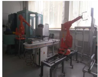
Management and Technological Engineering, of University of Oradea. The flexible cell consists of one CNC machine, two ABB robots for loading and unloading operations, two Pallets for part transfer, conveyor and storage area for raw parts and finished parts. Here, five
different parts have been machined in the cell to collect real processing time and those parts are implemented in this Hierarchical timed colored model for simulation.
Fig. 1. Flexible Manufacturing Cell from Faculty of Management and Technological Engineering, University
of Oradea.
3. DESIGN PARAMETERS FOR THE CELL
To construct the hierarchical model the significant meaning of resources in places, action in all transitions and their characteristics are mentioned in table 1 and table 2.
Table 1
PLACE POSITION IN CELL Places Characteristics
P1 Storage area for raw parts. P2 Robot1.
P3 Part is near pallet1.
P4 Pallet1 (used for raw parts). P5 Raw part is on the pallet1. P6 Raw part near robot2. P7 Robot2.
P8 Raw part is near the machine. P9 Machine.
P10 Part is in the machine. P11 Tool allocation. P12 Part is in processing.
P13 Part is finished and waiting for robot2. P14 Finished part near buffer2.
P15 Pallet2.
Table 2
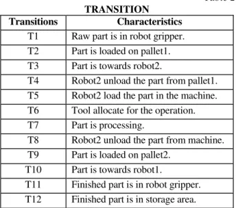
TRANSITION Transitions Characteristics
T1 Raw part is in robot gripper. T2 Part is loaded on pallet1. T3 Part is towards robot2.
T4 Robot2 unload the part from pallet1. T5 Robot2 load the part in the machine. T6 Tool allocate for the operation. T7 Part is processing.
T8 Robot2 unload the part from machine. T9 Part is loaded on pallet2.
T10 Part is towards robot1.
T11 Finished part is in robot gripper. T12 Finished part is in storage area.
4. COLOR AND VARIABLE DEFINITION FOR THE CELL
The color set for five different parts with time: (colset piece = with P1|P2|P3|P4|P5 timed): piece = {1`P1@336; 1`P2@458;
1`P3@1148; 1`P2@2160; 1`P2@2460}.
Colors defined for ABBrobot1 (P2): (colset robot = with R1 timed): Robot = {1`R1@0},
Colors defined for ABBrobot2 (P7): (colset robot= with R2 timed): Robot = {1`R1@0}.
Colors defined for Machine (P9): (colset machine = with M1): Machine = {1`M1}.
Colors defined for Pallet1 (P4): (colset pallet1 = with B1): Machine = {1`B1@0}, Colors define for Pallet2 (P15): (colset pallet2 = with B2): Machine = {1`B2@0}.
The color set for all five different parts and the color set for robot1 combined together in place P1 according to part arrival time, so in place P1 the complex color is denoted as colset product1 = (product piece*robot1 timed) 1`(P1,R1)@0++1`(P2,R1)@600++1`(P3,R1)@ 1500++1`(P4,R1)@2800++1`(P5,R1)@4000. The sequence of part arrival times follows the shortest processing time criteria. When the parts are released from place P1 for longest processing time it follows the sequences 1`(P5,R1)@0++1`(P4,R1)@2600++1`(P3,R1) @5000++1`(P2,R1)@6300++1`(P1,R1)@6900.
The color set is defined for pallet1 as product2 = (product piece*pallet1 timed) and
the color set is defined for pallet2 as product 6 = (product piece*pallet2 timed). Product 2 and product 6 represent the complex color for piece and pallet. The color set is defined for robot1 as product1 = (product piece*robot1 timed) and the color set is defined for robot2 as product 3 = (product piece*robot2 timed). Product1 and product3 represent the complex color for piece and robot. The product and robot1 have this complex color pairs in order to run the system. This can be defined by: {P1, R1}, {P2, R1}, {P3, R1}, {P4, R1}, {P5, R1} and {P5, R1}, {P4, R1}, {P3, R1}, {P2, R1}, {P1, R1}.
Color definitions for Variables: In Color Petri Nets connections are established between places and transitions defined by arcs. In this model arcs are assigned with the variables to
create connections between places and
transitions.
The variable for parts is defined by “p” and it has the color values (P1, P2, P3, P4, and P5).
} 5 P , 4 P , 3 P , 2 P , 1 P { p∈
The variables for robot1 (R1) and robot2 (R2) are “r1” and “r2”.
} 1 R { 1 r ∈ } 2 R { 2 r ∈
The variable for machine can be defined by “m1” which has color value:
} 1 M { 1 m ∈
The variables for pallet1 and pallet2 can be defined by “b1” and “b2” which has the color value: } 1 B { 1 b ∈ } 2 B { 2 b ∈
The model must create connections between the parts and machine in colored petri nets through the variables which were mentioned in arcs to establish the system.
} 1 M , 5 P }{ 1 M , 4 P }{ 1 M , 3 P }{ 1 M , 2 P }{ 1 M , 1 P { ) m p ( × ∈ } 1 M , 1 P }{ 1 M , 2 P }{ 1 M , 3 P }{ 1 M , 4 P }{ 1 M , 5 P { ) m p ( × ∈
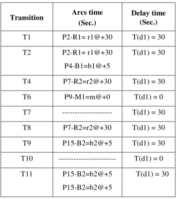
specific places to define the quantity of parts, machine, robots and pallets. Below in table 3 we present the initial token position and in table 4 we present the times related to arcs and delay in the cell with respect to mentioned transitions.
Table 3
TOKEN POSITIONS IN CELL
Places Token position Token Amount
P1 (P1,R1),(P2,R1),(P3,R1), (P4,R1), (P5,R1) or (P5,R1),(P4,R1),(P3,R1),
(P2,R1), (P1,R1)
5
P2 R1 1
P4 B1 1
P7 R2 1
P9 M1 1
P11 T1 1
P15 B2 1
Table 4
ARCS AND DELAY TIMES IN CELL
Transition Arcs time (Sec.)
Delay time (Sec.)
T1 P2-R1= r1@+30 T(d1) = 30 T2 P2-R1= r1@+30
P4-B1=b1@+5
T(d1) = 30
T4 P7-R2=r2@+30 T(d1) = 30 T6 P9-M1=m@+0 T(d1) = 0 T7 --- T(d1) = 30 T8 P7-R2=r2@+30 T(d1) = 30 T9 P15-B2=b2@+5 T(d1) = 30 T10 --- T(d1) = 0 T11 P15-B2=b2@+5
P15-B2=b2@+5
T(d1) = 30
5. HIERARCHICAL MODEL OF THE CELL
The hierarchical timed Color Petri Nets (HTCPN) formalism provides extension of
structured model with coloring, time
representations, hierarchy, priority in transitions etc. In CPN Tools color, time and hierarchy representations are the important feature to build the structure.
In this model we used CPN Tools to construct a single machine cell extension with time and hierarchy. The base model contains storage area for raw and finish parts, for loading and unloading operation performed by two robots, two pallets used for transport of raw parts and finished parts through the conveyor and a single machine for processing the parts.
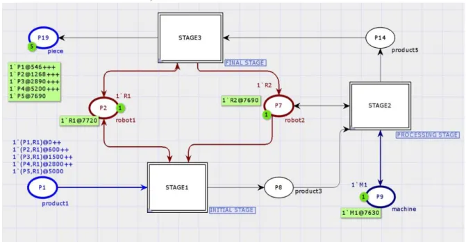
The basic model contains three sub models respectively: (a) initial stage, (b) Processing stage, (c) Final stage model.
In case1: The parts are released from resources with the time span respectively: P1 with 0 seconds, P2 with 600 seconds, P3 with 1500 seconds, P4 with 2800 seconds and P5 with 5000 seconds. This follows the shortest processing time (SPT) rules in transition T6.
In case2: parts are released from resources with time stamp respectively: P5 with 0 seconds, P4 with 2600 seconds, P3 with 5000 seconds, P2 with 6300 seconds and P1 with 6900 seconds with longest processing time sequence in transition T6.
Fig. 2. Part arrival time appear in hierarchical flexible cell based on LPT rules.
P1
product1 1`(P1,R1)@0++ 1`(P2,R1)@600++ 1`(P3,R1)@1500++ 1`(P4,R1)@2800++ 1`(P5,R1)@5000
P7
robot2 1`R2
P9
machine 1`M1
P8
product3
P14
product5
P19
piece
P2
robot1 1`R1
STAGE1
INITIAL STAGE INITIAL STAGE
STAGE2
PROCESSING STAGE PROCESSING STAGE
STAGE3
FINAL STAGE FINAL STAGE
P1 = P1 P8 = P8 P7 = P7 P2 = P2
P7 = P7 P14 = P14 P8 = P8 P9 = P9 P2= P2
P7= P7 P19 = P19 P14 = P14
Fig. 3. Part arrival times appear in Base model of hierarchical flexible cell based on SPT rules.
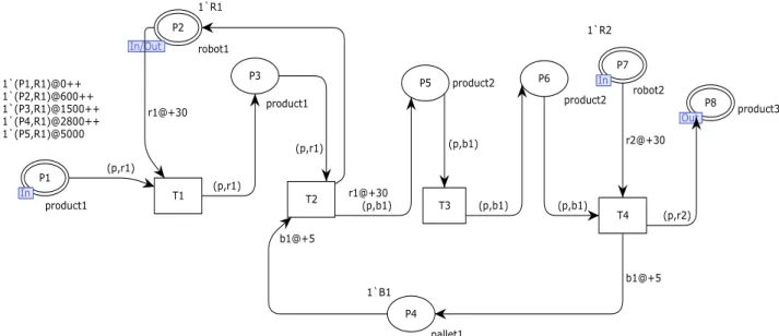
5.1 MODEL OF INITIAL STAGE
The complex color “product1” refers to an input function and color “robot1” to an input and output function associated with transition T1. Place1 and Place2 are combined with variable (p, r1) and arrival time span of all parts declared with set of colors according to SPT priority rule, respectively: (P1, R1), (P2, R1), (P3, R1), (P4, R1), (P5, R1) and LPT priority rule, respectively: (P5, R1), (P4, R1), (P3, R1), (P2, R1), (P1, R1). In place P1, the decision is declared with part arrival time, so robot1 load the part according to the mentioned command.
Pallet1 is associated with color set “B1” with delay time b1@+30 seconds and arc timing b1@+5 seconds. Robot2 also refers to an input function in the system with color set “R2” including arc timing with r2@+30 seconds. Complex color “product3” works as an output function for the phase 1. In stage 1, places P1 to P8 and transition T1 to T4 are connected through 13 arcs with time. Transition T2 and T4 are associated with delay time @+30 seconds. Complex color “product1” and “product2” are combined in place3 and place 4 with variables.
P3
product1
P4 pallet1 1`B1
P5 product2 P6
product2
P1 In
product1 1`(P1,R1)@0++ 1`(P2,R1)@600++ 1`(P3,R1)@1500++ 1`(P4,R1)@2800++ 1`(P5,R1)@5000
In
P8
Out product3 Out
P7 In
robot2 1`R2
In P2
In/Out robot1 1`R1
In/Out
T1 T2
T3
T4 (p,r1)
(p,b1) (p,b1)
b1@+5
(p,b1)
b1@+5 (p,r1)
(p,b1) (p,r1)
(p,r2) r2@+30
r1@+30 r1@+30
In Figure 4 we present the inside view of initial stage with all input and output functions for priority rule SPT. The inside view for the LPT rule based model are similar only in place P1 part arrival time is different.
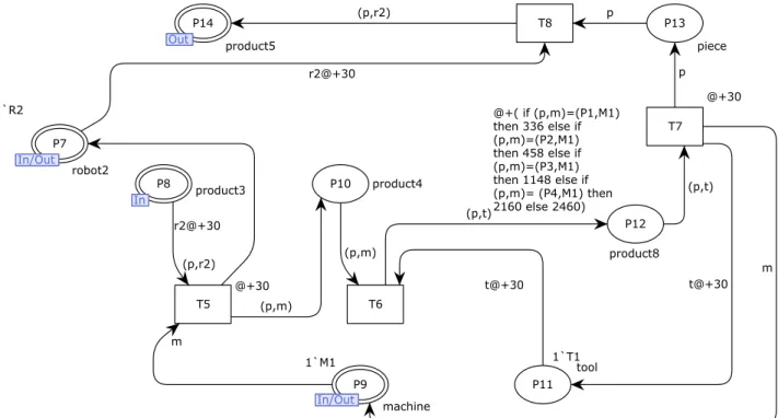
5.2 MODEL OF PROCESSING STAGE
The construction of the processing stage is associated with robot2, machine and tools. Place 8 with complex color “product3” is set as an input function, robot2 as an input and output function and the machine is also set as an input and output function. The total output of this section is obtained in place 14 with complex color “product5”. The machine is associated with color “M1” and the tool with “T1” through transition T6. In this stage in total 8 places and 4 transitions are connected using 14 arcs. Robot2 and the tool are associated with arcs with time respectively r2@+30 and t1@+30 in seconds. Time delay is also considered at transition T5 and T7 respectively @+30 seconds. Variables associated with robot2, machine and tool are mentioned in respective arcs combining with piece variable “p” as (p, r2), (p, m) and (p, t). Place 12 with complex color “product 8” refers to a part processing
place to perform machining operation for all five parts. Place13 with complex color “piece” is associated with delay time @+30 with transition T7 to describe the notation of part processing finish and transition T8 with delay
time @+30 is associated with robot2
performing unloading operation and transfer to the pallet2. Also, Transition T8 provides the output function connected with arc variables (p, r2) to place P14. In transition T5, robot2 load the part in the machine with delay time @+30 seconds.
When the part is appearing in transition T6, all five parts are processed from the minimum processing time to the maximum processing time in system. The decisions will follow the SPT rules for parts: if (p, m) = (P1, M1) then 336 else if (p, m) = (P2, M1) then 458 else if (p, m) = (P3, M1) then 1148 else if (p, m) = (P4, M1) then 2160 else 2460.
In transition T6, the parts are processed from the maximum processing time to the minimum processing time. The decision in T6, follow LPT priority rule. The following decision sequence is: if (p, m) = (P5, M1) then 2460 else if (p, m) = (P4, M1) then 2160 else if (p, m) = (P3, M1) then 1148 else if (p, m) = (P2, M1) then 458 else 336.
P10 product4
P11 tool 1`T1
P12
product8 P13
piece
P7
In/Out
robot2 1`R2
In/Out
P14
Out product5 Out
P8
In product3
In
P9
In/Out
machine 1`M1
In/Out
T5
@+30
T6
@+( if (p,m)=(P1,M1) then 336 else if (p,m)=(P2,M1) then 458 else if (p,m)=(P3,M1) then 1148 else if (p,m)= (P4,M1) then 2160 else 2460)
T7
@+30 T8
(p,m)
p
(p,t)
t@+30 (p,m)
p
(p,t)
t@+30 r2@+30
(p,r2)
(p,r2)
m
r2@+30
m
Fig. 6. Inside view of processing stage of flexible manufacturing cell implement of LPT rule decision in T6 for.
In Fig.5 and Fig.6 the inside view are similar but the decision in transition T6 is different because the performance of machining for the models are different, due to the implementation of different priority rules respectively SPT and LPT. In the above Figures transition T6 contains the decision to perform operation sequence.
5.3 MODEL OF FINAL STAGE
The final stage contains robot1, robot2 and pallet2 and a place for finished part storage, in place P19. Place P14 refers to an input function, in this phase with complex color
“product 5”. Robot2 performs loading
operation for pallet2 in this section, so it’s mentioned as an output functions. The delay time is @+30 seconds in transition T2 which make the connection between pallet2 and robot 2. The part transfer time for pallet2 is considered in arc time with b2@+5 seconds.
Transition T11 combines with robot1 and pallet2 with delay time @+30 seconds with arc time r1@+30 seconds. Place P19 describes a final storage area for finished part with complex “color” piece. In this section a total of 8 places and 4 transitions are connected through 13 arcs to construct the section. Here, pallet2 is considered to perform the transfer of finished parts from transition T9 to transition T11. Place 16 and 17 is associated with complex color “product6” and place P18 is associated with
complex color “product7” to establish
connection with both robots and pallets.
P16 product6 P17
product6 P15
pallet2 1`B2 P18
product7
P2
In/Out robot1
1`R1
In/Out
P7
Out
robot2 1`R2
Out
P19
Out
piece
Out
P14
In
product5
In
T9
@+30
T10 T11
@+30 T12
(p,b2) (p,b2)
(p,r1)
(p,b2) b2@+5 (p,r1)
b2@+5
(p,b2) r1@+30
r2@+30 r1@+30
p
(p,r2)
Fig. 7. Inside view of Final stage configuration of the flexible manufacturing cell.
6. SIMULATION AND OBSEVATION OF THE CELL OPERATION
In this flexible cell, we are machining five different parts on a single machine with part arrival times for two different priority rules. Place P1 contains all five parts with token
is now in robot1 gripper. At delay time @+30, robot1 unload the part in the pallet1 and robot 1 moves back to place P2. The status of robot1 is now free. The part is now in pallet1 to transfer near robot2 through complex color “product2”. The part transfer time of pallet1 is b1@+5 seconds. The status of place P5, means that the part is on the pallet and place P6 describe that the part is near robot2. So, robot 2, unload the part from pallet1 after delay time @+30 seconds and arcs timing r2@+30 seconds considers the robot moving time from place to transition. Pallet2 returns to its place after arc timing b1@+5 seconds and now it’s free. After, enabling transition the part is moving at complex color “product 3” which is the output function of the initial stage.
In the processing stage the parts are processed according to priority rules. When using SPT priority rules the transition T6 follows the decision tree: if (p, m) = (P1, M1) then 336 else if (p, m) = (P2, M1) then 458 else if (p, m) = (P3, M1) then 1148 else if (p, m) = (P4, M1) then 2160 else 2460. When we implement LPT priority rules in transition T6, it follows the decision tree: if (p, m) = (P5, M1) then 2460 else if (p, m) = (P4, M1) then 2160 else if (p, m) = (P3, M1) then 1148 else if (p, m) = (P2, M1) then 458 else 336. All those parts are processed enabling transition T6 in place P12. Place P13 shows the part is finished and the tool and machine return back to their place with token. At transition T8, the robot is
ready to unload the finished part from the machine, adding arc time with r2@+30 seconds. In this condition part is in robot2 gripper at place P14 which is the output for
processing stage. At the enabling of transition T9, the firing is active and robot2 unload the finished part in pallet2 to transfer through the conveyor. Here, also arc time for pallet2 is considered to be b1@+5 seconds to transfer the part.
In the final stage, robot2 is loading the part in pallet2, and then returns back in its place with token. As usual, place P16 and place P17 shows “the part is on the pallet” and “part is near robot1”. Conditions are made in this system in such a manner that robot1 should be free for unload the part from pallet1 before load the second part in the machine. So, at transition T1, after 30 seconds robot1 unload the part from pallet2 and pallet2 return in place P15 with token 1. Now, the finished part is ready to be delivered in the final storage area at Place P19 after firing at transition T12. Only the part is appearing in place P19 with variable “p” and robot1 returns in its place P2 to perform the next operation.
The results observed from the simulation appear in the base model and final stage model of the cell in place P2, P7, P9 and P19 and also each sub model contain the results in mentioned places. During simulation when the sub model is active it shows a green line.
Total time = part arrival time + delay time + arc time + machining time.
During simulation the current time in each place is shown to define the exact time for a particular place. Each time the movement of token is observed for all parameters. If a place is free the token is available if it is busy the token moves from that place.
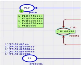
After simulation in place P19 the total time found for SPT rules is 7690 seconds and for LPT rules it took 7446 seconds. From observation of SPT and LPT rules it is found that the total time for releasing a part from place P1 according to LPT is more time saving compare to SPT. The time difference is found to be 244 seconds after processing all five parts in the cell.
Fig. 9. Total time appears in Base model of a flexible manufacturing cell after simulation according to LPT rules.
Table 5
TOTAL TIME (SPT) AND (LPT)
Part Total time (TT) seconds Part Total time (TT) seconds
P1 546 P5 2690
P2 1268 P4 4970
P3 2890 P3 6390
P4 5200 P2 6990
P5 7690 P1 7446
8. CONCLUSION
In this paper, we explained the modeling and simulation of FMC implemented with HCTPN formalism using CPN Tools. The contribution of the work is modeling and simulation of single machine flexible cell with decision based priority activation in transition. Also, the parts are released from resources according to minimum to maximum processing time (SPT) and maximum to minimum processing time (LPT) to perform the operation. The decision is declared in transition to follow the priority rules. The observed results highlighted that LPT rules are more effective than SPT.
9. REFERENCES
[1] P. Huber, K. Jensen and R.M. Shapiro,
“Hierarchies in coloured petri nets”. In:
Rozenberg G. (eds) Advances in Petri Nets 1990. ICATPN1989. Lecture Notes in Computer
Science, vol. 483, Springer, Berlin, Heidelberg, 1991.
[2] M.C.Zhou, K. McDermott, P.A. Patel, “Petri net synthesis and analysis of a flexible
manufacturing system cell”. IEEE Transactions
on Systems, Man, and Cybernetics, vol. 23, issue 2, pp.523–531, 1993.
[3] Z. Ye, T. Wang and P. Sun, “A petri net based approach for flexible manufacturing system
modeling” International Conference on
Automatic Control and Artificial Intelligence,
ISBN: 978-1-84919-537-9, pp. 252 –254, 3-5
march,Publisher:IET, 2012.
[4] L. C. Wang and S. Y. Wu, “Modeling with colored timed object-oriented Petri nets for
automated manufacturing systems”. Computers
and Industrial Engineering, vol. 34, issue2, pp.463-480, 1998.
[5] J. Chen, F.F. Chen, “Performance modelling and evaluation of dynamic tool allocation in flexible manufacturing systems using Coloured Petri nets: an object-oriented approach”.
[6] H. Van Brussel, Y. Peng, P. Valckenaers, “Modelling Flexible Manufacturing Systems
Based on Petri Nets” CIRP Annals -
Manufacturing Technology Vol. 42, Issue 1, pp.479–484,1993.
[7] E. R. R. Kato, O. Morandin Jr., M. Sgavioli “A
Conflict Solution Manufacturing System
Modeling using Fuzzy Coloured Petri Net”
Systems Man and Cybernetics (SMC), IEEE International Conference on Istanbul, pp.3983 – 3988, 2010.
[8] K. Abd, K. Abhary, R. Marian, “A Methodology for fuzzy multiple criteria decision making approach for scheduling problems in robotic
flexible assembly cells” IEEE International
Conference on Industrial Engineering and Engineering Management, pp.374 – 378, 2014. [9] S. T. F. Chan, B. Rajat, C. K. Hing, “The effect
of responsiveness of control-decision system to
the performance of FMS”, Computer and
Industrial Engineering, vol. 72, pp.32-42, 2014. [10] F. Blaga, I. Stanasel, A. Pop, V. Hule and T.
Buidos, “Consideration on flexible
manufacturing cell modeling with timed
coloured petri nets” ANNALS OF THE
ORADEA UNIVERSITY, Fascicle of Management and Technological Engineering , Issue #1, May 2014, pp 299- 302, http://www.imtuoradea.ro/auo.fmte.
[11] M.G. Abou-Ali, M.A. Shouman, “Effect of dynamic and static dispatching strategies on dynamically planned and unplanned FMS”
Journal of Materials Processing Technology, vol. 148, pp.132–138, 2004.
[12] F. B. Reis, V. F. Carida, O. Morandin, R. L.
Castro, C. CM. Tuma “A Colaborative Fuzzy
CPN System for Conflict Solution of Flexible
Manufacturing System” Industrial Electronics
Society, IECON 2013 - 39th Annual Conference of the IEEE , pp.3216 – 3221, ISBN-978-1-4799-0223-1, Vienna , 10-13 Nov, 2013.
[13] A. Zimmermann; G. Hommel, “Modelling and Evaluation of Manufacturing Systems Using
Dedicated Petri Nets”. Int. Journal of Advanced
Manufacturing Technology; Special Issue on Petri Nets Applications, Band 1/15/1900, pp. 132-137, Springer- Verlag, Berlin, 1999.
[14] N. Viswanadham and Y. Narahari, “Coloured petri net models for automated manufacturing
systems” Proc. IEEE Int. Conf. Robot. Automat,
vol.4, pp.1985-1990, 1987.
[15] K. P. Valavanis, “On the hierarchical modeling analysis and simulation of flexible manufacturing systems with extended Petri
nets”. IEEE Transactions on Systems, Man, and
Cybernetics, vol.20, issue1, pp.94–110, 1990.
APLICAREA REGULILOR DE PRIORITATE IN SIMULAREA CELULELOR FLEXIBILE DE FABRICATIE UTILIZAND MODULE IERARHICE CU RETELE PETRI
COLORATE TEMPORIZATE
Abstract: Această lucrare are ca obiectiv modelarea şi simularea unei cellule flexibile de fabricaţie utilizând modele ierarhice bazate pe reţele Petri Colorate Temporizate. Ȋn cadrul celulei flexibile sunt prelucrate diferite tipuri de piese corespunzător deciziilor modelate prin tranziţii, regula de prioritate fiind data de timpii de prelucrare. Modelul realizat are la bază o celulă flexibilă de fabricaţie de la Facultatea de Inginerie şi Manageriala a Universităţii din Oradea. Procedura propusă permite evaluarea indicatorilor de performanță ai celulei, informațiile obținute pot fi utilizate in luarea deciziilor în planificarea producţiei.
Sanjib Kumar SAREN, PhD student, Mechatronics Department, University of Oradea, Str. Universităţii nr. 1, Oradea, 410087, Bihor, email: [email protected], +40731651063.
Florin BLAGA, prof. Eng. Industrial engineering, University of Oradea, Str. Universităţii nr. 1, Oradea, 410087, Bihor, email: [email protected].