TECHNICAL UNIVERSITY OF CLUJ-NAPOCA
ACTA TECHNICA NAPOCENSIS
Series: Applied Mathematics, Mechanics and Engineering Vol. 62, Issue II, June, 2019
CONSIDERATIONS ABOUT ALGEBRAIC FITTING OF AN ELLIPSE TO
SCATTERED 2D DATA
Nicolae URSU-FISCHER
Abstract: The our aim of this work is to present some theoretical aspects and numerical results about the algebraic ellipse fitting to 2D data, showing the advantages and also the drawbacks of this procedure. All the necessary theoretical aspects are rigorously presented, as well as many examples that justify the usefulness of the method of algebraic fitting. Consulting the graphical obtained results, one may notice that the accuracy corresponds for the practical use of this method. Consulting the literature, we observe that the main part of scientific works deal with the geometric fitting and the algebraic fitting is considered only to show its deficiencies with respect to the geometric fitting. Our hope is that the algebraic fitting will be reconsidered and used in the cases when it is applicable.
Key words: ellipse, algebraic fitting, least-squares method, parametric equations, accuracy
1. INTRODUCTION
The fitting of curves or surfaces to 2D or 3D data is a current research subject in different fields of science and engineering, especially when the curve is a circle or ellipse and is a relevant subject in coordinate metrology, computer aided design and computer/machine vision.
In 1901, the Pearson’s paper [12] was published, where one may find the basic problems that have to be solved to accomplish the fitting problem.
In present days the fitting of simple primitives (lines, circles, ellipses) to data obtained experimentally, is one of the basic problem in computer vision and pattern recognition.
There are two different methods to obtain the analytical equations of desired curves: algebraic fitting and geometric fitting, each of them having advantages and drawbacks.
The algebraic fitting allows the computing of curve parameters which minimize the sum of square equation values at each given point. When one uses geometric fitting the values of curve parameters will minimize the sum of squared distances between the given points and
the curve. The geometric fitting is also named “best fit”.
Studying the literature one notices the existence of a great number of scientific papers dealing with circle fitting, the main problems being solved during the last 40-50 years, the methods belonging to I. Kåsa, V. Pratt and G. Taubin ([10], [13], [17]) are well known, being the starting point for future achievements in this domain.
The ellipse fitting – algebraic and geometric – was also intensively studied, existing many important papers, published by Sung Joon Ahn [1], [2] [3], Fred Bookstein [4], Andrew Fitzgibbon [5], Walter Gander [6], Kenichi Kanatani [7], [8], [9], Paul Rosin [15], [16], Hao Wang [21], G. A. Watson [22], [23] and many others.
This work is presenting some considerations and problems about the algebraic fitting of an ellipse to 2D data, showing the procedure to obtain valuable numerical results, the resulting ellipses performing a good fitting to the given 2D data.
- the values of semi-major and semi-minor axes, the coordinates of the ellipse center, pose angle (rotation angle between the major axis and horizontal line), or
- the two ellipse foci coordinates and the length of semi-major (or semi-minor) axis. Some numerical examples are done for justifying the proposed procedure and for showing the correctness of the obtained results.
2. THE GENERAL FORM OF ELLIPSE EQUATION DETERMINATION
A number of m points with known coordinatesP1(x1,y1),.., Pk(xk,yk),
) y , x ( P , .
. m m m are given, in the plane Oxy, as
shown in figure 1
Fig. 1. The points to be fitted with an ellipse The scope is to find the equation of an ellipse that fits the given points in the sense of algebraic fitting.
The following equation has to be obtained
0 F y E 2 x D 2 y C y x B 2 x
A 2 + + 2 + + + = (1) which represents the general equation of a conic. Reducing to five the number of parameters, dividing the equation by A (A≠0) and noting
A / F F , A / E E , A / D D , A / C C , A / B B * * * * * = = = = =
the equation becomes
0 F y E 2 x D 2 y C y x B 2
x2 + * + * 2 + * + * + * = (2) The sum of “algebraic distances” is
2 * k * m 1 k k * k k * 2 k * 2 k ) F y E 2 x D 2 y x C 2 y B x ( E + + + + + + =
= (3)
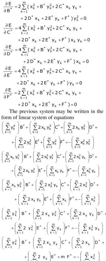
and its minimal value will be obtained for the parameter values obtained after solving the following simultaneous equations, according to the method of least squares,
0 y ) F y E 2 x D 2 y x C 2 y B x ( 2 B E 2 k * k * k * m 1 k k k * 2 k * 2 k * = + + + + + + = ∂ ∂
= 0 y x ) F y E 2 x D 2 y x C 2 y B x ( 4 C E k k * k * k * m 1 k k k * 2 k * 2 k * = + + + + + + = ∂ ∂
= 0 x ) F y E 2 x D 2 y x C 2 y B x ( 4 D E k * k * k * m 1 k k k * 2 k * 2 k * = + + + + + + = ∂ ∂
= 0 y ) F y E 2 x D 2 y x C 2 y B x ( 4 E E k * k * k * m 1 k k k * 2 k * 2 k * = + + + + + + = ∂ ∂
= 0 ) F y E 2 x D 2 y x C 2 y B x ( 2 F E * k * k * m 1 k k k * 2 k * 2 k * = + + + + + + = ∂ ∂
=The previous system may be written in the form of linear system of equations
− = + + + + +
= = = = = = m 1 k 2 k 2 k * m 1 k 2 k * m 1 k 3 k * m 1 k 2 k k * m 1 k 3 k k * m 1 k 4 k y x F y E y 2 D y x 2 C y x 2 B y − = + + + + + = = = = = = m 1 k k 3 k * m 1 k k k * m 1 k 2 k k * m 1 k k 2 k * m 1 k 2 k 2 k * m 1 k 3 k k y x F y x E y x 2 D y x 2 C y x 2 B y x − = + + + + +
= = = = = = m 1 k 3 k * m 1 k k * m 1 k k k * m 1 k 2 k * m 1 k k 2 k * m 1 k 2 k k x F x E y x 2 D x 2 C y x 2 B y x − = + + + + +
= = = = = = m 1 k k 2 k * m 1 k k * m 1 k 2 k * m 1 k k k * m 1 k 2 k k * m 1 k 3 k y x F y E y 2 D y x 2 C y x 2 B y − = + + + + +
= = = = = m 1 k 2 k * * m 1 k k * m 1 k k * m 1k k k
* m 1 k 2 k x F m E y 2 D x 2 C y x 2 B y
and solved with the method of partial or total pivoting [14], [18] a. o. The values of B* , C* , D* , E* and F* will result. The type of conic that may be obtained depends on the value of the expression AC-B2 if the ellipse has the equation (1), or * * 2
] B [
< = > −
hyperbola ,
0
parabola ,
0
ellipse ,
0 B C
A 2
* * 2
] B [ C −
< = >
hyperbola ,
0
parabola ,
0
ellipse ,
0
(4)
The following ellipse equation was obtained for the numerical values of given coordinates:
0 1428 . 1 y 0416 . 1 2 x 7641 . 0 2
y 66087 . 1 y x 6762 . 0 2
x2 2
= +
× − ×
−
− +
×
− (5)
After we have solved analytically the problem, computing the coefficient values of the general equation of ellipse, it is necessary to obtain the graphical image of the ellipse. Two ways are allowed to obtain this.
The shape of the ellipse may be visualized on the screen if the interior pixels are colored with different color than the background color. If there is a point having the coordinates [x0,y0] , considering the closed curve of implicit formf(x,y)=x2+2B*xy+ C*y2+2D*x+
0 F y E
2 * + *=
+ , three cases are possible, as follows:
< = >
int po erior int , 0
contour the
on , 0
int po exterior ,
0 ) y , x ( f 0 0
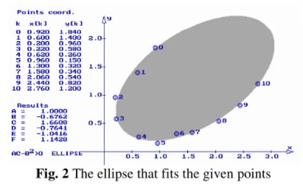
Considering an ellipse inscribed in a rectangle, for the rectangle points are computed the value of the function f(x,y), the condition is checked, if the point is interior the corresponding pixel is colored with a specified color. The obtained ellipse is shown in figure 2. .
Fig. 2 The ellipse that fits the given points Usually we have to obtain on the screen the solid curve as an ellipse contour.
The parametric equations of an ellipse are as follows [11] pp. 273,
− + =
= +
+ + +
−
− + −
=
) x x ( t y y
, 1 A , A t B 2 t C
) D y B 2 x A (
t ) E y C ( 2 t x C
x
E E
* 2 *
* E * E
* E * 2 E *
(6)
where xE and yE are the coordinates of some point belonging to the ellipse contour and the position of this point E has to be previously determined.
If the center of gravity G of the m given points is determined
= = =
= m
1 k
m
1 k
k G
k
G y
m 1 y , x m
1 x
it is obvious that each horizontal and vertical lines passing through point G will intersect the ellipse contour in two points.
Considering the vertical line x=xG two ordinate values will result after solving the equation
0 F y E 2 x D 2 y C y x B 2
x2G+ * G + * 2+ * G+ * + *=
0 F x D 2 x y ) E x B ( 2 y
C* 2+ * G + * + 2G+ * G+ *=
with roots
*
* G * 2 G *
2 * G * *
G *
2 , 1
C
) F x D 2 x ( C
) E x B ( ) E x B (
y − + +
− + ±
+ −
=
) y , x (
or ) y , x ( ) y , x (
2 G
1 G
E
E (7)
Now the ellipse contour may be represented as in figure 3.
Fig. 3 The contour of the ellipse that fits the given points 3. DETERMINATION OF OTHER
ELLIPSE EQUATIONS
The general equation of the fitting ellipse was established
0 F y E 2 x D 2 y C y x B 2 x
A 2 + + 2 + + + = (8) or
0 F y E 2 x D 2 y C y x B 2
noticing that the same ellipse is obtained if the equation is multiplied or divided with a constant.
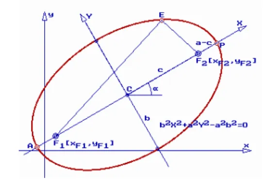
The ellipse is well defined if other five parameters are known: the lengths of semi-major and semi-minor axes, a and b, the ellipse centre C coordinates, xC , yC and the angle
α
between horizontal line and the major axis (figure 4). At this point the key question is to find the relations between the parameters B*, C*, D*, E* and F* and the ellipse elements a, b, xC , yC and
α
.Fig. 4. The ellipse and two coordinate frames Two coordinate frames were considered: in figure 4, Oxy and CXY. With respect to the second frame ellipse equations may be written in two ways, Cartesian and parametric,
b2 X2 +a2 Y2 −a2b2 =0 (10) X =acosϕ, Y =b sinϕ (11) The relations between ellipse coordinates depending of the considered frames may be written in matrix forms,
α α α − α + = Y X cos sin sin cos y x y x C C − − α α − α α = C C y y x x cos sin sin cos Y X or α + α + = α − α + = cos Y sin X y y sin Y cos X x x C C α − + α − − = α − + α − = cos ) y y ( sin ) x x ( Y sin ) y y ( cos ) x x ( X C C C
C (12)
Combining (10) with (12) it results
0 b a ] ) cos y sin x ( cos y sin x [ a )] sin y cos x ( sin y cos x [ b 2 2 2 C C 2 2 C C 2 = − − α − α + α + α − + + α + α − α + α
After some algebraic manipulation one obtains 0 ] sin ) x a y b ( cos ) y a x b ( ) b a ( y x cos sin 2 [ y ] ) sin b cos a ( y ) b a ( x cos sin [ 2 x ] ) cos b sin a ( x ) b a ( y cos sin [ 2 y ) cos a sin b ( y x ) a b ( cos sin 2 x ) sin a cos b ( 2 2 C 2 2 C 2 2 2 C 2 2 C 2 2 2 C C 2 2 2 2 C 2 2 c 2 2 2 2 C 2 2 c 2 2 2 2 2 2 2 2 2 2 2 2 = α + + + α + + + − α α − + + α + α − − − α α + + α + α − − − α α + + α + α + + − α α + + α + α (13)
and after identifying the coefficients of equations 0 F y E 2 x D 2 y C Y X B 2 x
A 2 + + 2+ + + =
and (13) will result
α +
α
=b2cos2 a2sin2
A (14)
) a b ( cos sin
B= α α 2− 2 (15)
α +
α
=b2sin2 a2cos2
C (16)
) cos b sin a ( x ) b a ( y cos sin D 2 2 2 2 C 2 2 c α + α − − − α α = (17) ) sin b cos a ( y ) b a ( x cos sin E 2 2 2 2 C 2 2 c α + α − − − α α = (18) α + + + α + + + − α α − = 2 2 C 2 2 C 2 2 2 C 2 2 C 2 2 2 C C sin ) x a y b ( cos ) y a x b ( ) b a ( y x cos sin 2 F (19)
Because relation (8) may by multiplied or divided with a constant, it results that the obtained values of a and b will be proportional to the real values of a and b.
From (14) and (16) one obtains
α − α α − α = 4 4 2 2 2 cos sin cos C sin A a α − α α − α = 4 4 2 2 2 cos sin cos A sin C b α − α α − α = 2 2 2 2 cos C sin A cos A sin C a
b (20)
and introducing the determined values in (15) will result C A B 2 2 tan − =
α ,
− = α C A B 2 tan a 2 1 (21)
The relations (17) and (18) may be considered as a system of two linear equations with unknowns xC and yC ,
E y ) sin b cos a (
x ) b a ( cos sin
D y ) b a ( cos sin
x ) cos b sin a (
C 2 2 2 2
C 2 2
C 2 2
C 2 2 2 2
= α +
α −
− −
α α
− = −
α α −
− α +
α
The two solutions are as follows
2 2
2 2
2 2 2 2
C
b a
cos sin ) b a ( E
) sin b cos a ( D
x + − α α
+ α +
α
−
= (22)
2 2
2 2
2 2 2 2
C
b a
cos sin ) b a ( D
) cos b sin a ( E
y + − α α
+ α +
α
−
= (23)
the obtained values being also correct, for the same reason.
One last problem remains to be solved: which is the exact value of semi-major axis length. According to figure 4
2 A C 2 A
C x ) (y y )
x ( A C P C
a= = = − + − (24)
therefore the coordinates of points A or P have to be determined.
The major-axis, containing the point C, intersects the ellipse contour in points A and P (figures 4 and 5).
Fig. 5. The fitting ellipse, the centre and the major axis The analytical equation of major axis is
) x x ( tan y
y− C= α − C and intersects the ellipse
whose equation is
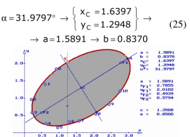
Ax2+2Bxy+Cy2 +2 Dx+2Ey+F=0. After solving the two degrees algebraic equation the coordinates of points A and P are known and result the length of semi-major axis a . The length of semi-minor axis b is obtained using the relation (20). The fitting ellipse and the two semi axes, the results being obtained in the following order:
8370 . 0 b 5891 . 1 a
2948 . 1 y
6397 . 1 x 9797
. 31
C C
= → =
→
→
= = →
° =
α
(25)
Fig. 6. The fitting ellipse, the centre, the major and minor axes and the results
The ellipse is also defined if other five values are known: coordinates of foci (xF1, yF1, xF2, yF2) and semi-major axis a. Using elementary calculi will result
c= a2 −b2 =1.3508 →
→
= α + =
= α +
= →
0102 . 2 sin c y y
7855 . 2 cos c x x
C 1 F
C 1 F
= α − =
= α −
= →
5794 . 0 sin c y y
4939 . 0 cos c x x
C 2 F
C 2
F (26)
One can notice that the algebraic fitting with an ellipse of the given points is successfully performed, the ellipse contour being very close to the points.
4. NUMERICAL EXPERIMENTS
` One example of fitting eleven point with an ellipse was completely presented during the explanations regarding the method.
In the following three more examples are presented, using different number of points and different arrangements of points in the plane. Only the graphical results will be shown.
Fig,. 8. Example 1. Second image
Fig. 9. Example 1. Third image
Fig. 10. Example 1. Fourth image
Fig. 11. Example 2. First image
Fig. 12. Example 2. Second image
Fig. 13. Example 2. Third image
Fig. 14. Example 2. Fourth image
Fig. 15. Example 3. First image
Fig. 16. Example 3. Second image
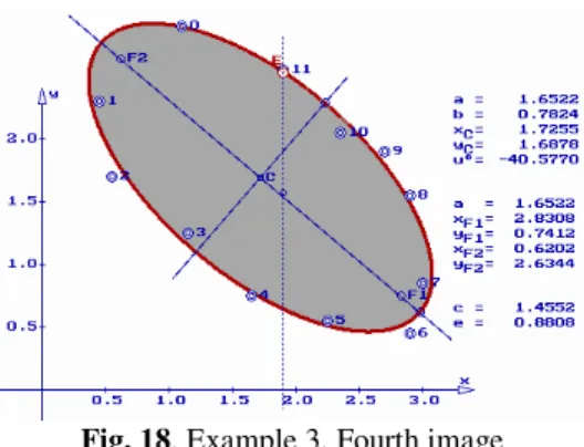
Fig. 18. Example 3. Fourth image
According to the presented examples, the fitting is performed with high accuracy, proving the efficiency of the implemented computer program..
5. CONCLUSIONS
The algebraic fitting of some given points in plane was studied by many researchers during the last years, together with the geometric fitting, each of the methods having advantages and also some drawbacks.
As previously shown, the analytical equation of ellipse is determined, using algebraic fitting, minimizing the sum of residual squares. The algebraic fitting error generally has no physical interpretation but the results are obtained quicker than in the case of geometric fitting, which involves iterative processes, sometimes with many steps.
In some cases the procedure ends in an unintended geometric figure, obtaining a hyperbola instead of an ellipse.
However, in many cases (and the presented cases are appropriate examples) the algebraic fitting may be used very successfully, the results being obtained quicker than for using geometric fitting.
One of the great advantages of algebraic fitting consists in the fact that is not necessary to start the procedure from some initial conditions, the number of formulas being the same, except the determination of coefficients of linear system with five equations and five unknowns. In the case of geometric fitting, the values of parameters used as initial data have a great influence on the necessary number of iterations
for obtaining the results with an imposed accuracy.
This research can be continued for comparing the results obtained for the same points in plane using both methods, computing for the algebraic fitting method the sum of squared distances between the points and the resulted ellipse.
6. REFERENCES
[1] Ahn, S. J., Rauh, W., Recknagel, M., Geometric fitting of line, plane, circle, sphere and ellipse, ABW-Workshop 3D-Bildverarbeitung an der Technischen Akademie Esslingen, 25-26 I 1999, 8 pp. [2] Ahn, S. J., Rauh, W., Warnecke, H.-J.,
Best-fit of implicit surfaces and plane curves, in Tom Lyche and Larry L. Schumaker (eds.), Mathematical Methods for Curves and Surfaces, pp. 1-14, Oslo, 2000, ISBN 0-8265-1378-6
[3] Ahn, S. J., Rauh, W,., Warneke, H.-J., Least-squares orthogonal distances fitting of circle, ellipse, hyperbola and parabola, Pattern Recognition, 2001, Vol. 34, No. 12, pp. 2283-2303
[4] Bookstein, F. L., Fitting conic sections to scattered data, Computer Graphics and Image Processing, 1979, vol. 9, pp. 56-71 [5] Fitzgibbon, A., Pilu, M., Fisher, R. B., Direct
least square fitting of ellipses, IEEE Transactions on Pattern Analysis and Machine Intelligence, 1999, Vol. 21, No. 5, pp. 476-480
[6] Gander, W., Golub, G. H., Strebel, R., Least-squares fitting of circles and ellipses, BIT 1994, Vol. 34, pp. 558-578
[7] Kanatani, K., Ellipse fitting with hyperaccuracy, IEICE Trans. Inform. Syst., 2006, E89-D, pp. 2653–2660.
[8] Kanatani, K., Sugaya, Y., Compact algorithm for strictly ML ellipse fitting, Proceedings of 19th International Conference in Pattern Recognition, Tampa, FL., U.S., 2008
[10] Kåsa, I., A circle fitting procedure and its error analysis, IEEE Transactions on Instrumentation and Measurement, 1976, Vol. 25, pp. 8-14
[11] Murgulescu, Elena a. o., Analytical and Differential Geometry, sec. ed. (in Romanian), Editura Didactică şi Pedagogică, Bucureşti, 1965, 772 pp. [12] Pearson, K., On lines and planes of closest
fit to systems of points in space, The Philosophical Magazine, 1901, Ser. 6, Vol. 2, No. 11, pp. 559-572
[13] Pratt, V., Direct least-squares fitting of algebraic surfaces, Computer Graphics, 1987, Vol. 21, pp. 145–152
[14] Press, W. H. a. o., Numerical Recipes in C++. The Art of Scientific Computing, Cambridge University Press, 2003, 1002 pp., ISBN 0-521-75033-4
[15] Rosin, P. I., A note on the least square fitting of ellipses, Pattern Recognition Letters, 1993, Vol. 14, pp. 799-808
[16] Rosin, P. I., Analyzing error of fit functions for ellipses, British Machine Vision Conference, Pattern Recognition Letters, 1996, Vol. 17, No. 14, pp. 1461-1470 [17] Taubin, G., Estimation of planar curves,
surfaces and nonplanar space curves defined by implicit equations, with applications to edge and range image
segmentation, IEEE Transactions on Pattern Analysis and Machine Intelligence, 1991, Vol. 13, No. 11, pp. 1115–1138
[18] Ursu-Fischer, N., Ursu, M., Numerical Methods in Engineering and Programs in C/C++ (in Romanian), vol. I, Cluj-Napoca, Casa Cărţii de Ştiinţă, 2000, 282 pp., ISBN 973-686-039-6
[19] Ursu-Fischer, N., Ursu, M., Numerical Methods in Engineering and Programs in C/C++ (in Romanian), vol. II, Cluj-Napoca, Casa Cărţii de Ştiinţă, 2003, 288 pp., ISBN 973-686-463-4
[20] Ursu-Fischer, N., Ursu, M., A new and efficient method to perform the circle fitting, Acta Technica Napocensis, Series: Applied Mathematics and Mechanics, 2004, No. 47, Vol. III, pp. 21-30, ISSN 1221-5872 [21] Wang, Hao a. o., Robust real-time ellipse
fitting based on Lagrange programming neural network and locally competitive algorithm, IEEE Transactions, 2018, 30 pp. [22] Watson, G. A., Least squares fitting of circles and ellipses to measured data, BIT, 1999, Vol. 39, No. 1, pp. 176-191
[23] Watson, G. A., Least squares fitting of parametric surfaces to measured data, ANZIAM J., 42(E), pp. C68-C96
CONSIDERAŢII PRIVIND APROXIMAREA ALGEBRICĂ CU O ELIPSĂ A UNOR PUNCTE DIN PLAN Rezumat: Scopul acestei lucrări este de a prezenta principalele aspecte teoretice şi rezultate numerice privind aproximarea algebrică cu elipse a unor puncte dispuse în plan, arătând atât avantajele cât şi dezavantajele acestui procedeu. Toate aspectele teoretice sunt riguros prezentate, de asemenea un număr mare de exemple care justifică
utilitatea acestei metode de aproximare. Din reprezentările grafice obţinute se poate constata că precizia rezultatelor este corespunzătoare pentru ca metoda să poată fi folosită în diferite cazuri practice. Studiind literatura tehnică din domeniu se poate constata că majoritatea lucrărilor tratează problema aproximării geometrice iar cea algebrică este mai puţin utilizată. Scopul acestei lucrări este ca aproximarea algebrică să fie reconsideratăşi să fie utilizată în acele cazuri când se pot obţine în mod eficient rezultate, cu un număr minim de calcule .