Sharif University of Technology
Scientia IranicaTransactions A: Civil Engineering www.scientiairanica.com
Resilience of civil infrastructure by optimal risk
mitigation
M. Mahsuli
Department of Civil Engineering, Sharif University of Technology, Tehran, Iran.
Received 8 November 2014; received in revised form 26 May 2015; accepted 25 August 2015
KEYWORDS Risk mitigation; Infrastructure; Resilience; Seismic risk; Reliability method; Probabilistic model; Sensitivity.
Abstract.This paper puts forward a framework for optimal mitigation of regional risk to enhance the resilience of civil infrastructure. To meet this objective, probabilistic models, methods, and software are developed and applied. The work is conducted within a new reliability-based approach, in which reliability methods compute risk. This contrasts several contemporary approaches for risk analysis. Risk, in this context, denotes the probability of exceeding monetary loss. Evaluating such probabilities requires probabilistic models for hazards, response, damage, and loss. This motivates the following contributions in this paper. First, a new computer program is developed that is tailored to conduct reliability analysis with many interconnected probabilistic models. It orchestrates the interaction of models through an object-oriented architecture. Second, a library of probabilistic models for regional seismic risk analysis is developed. The library includes new models for earthquake location and magnitude and building response, damage, and loss. Third, probabilistic methods for multi-hazard risk analysis are developed and applied in a large-scale regional analysis. The results are cost exceedance probabilities and insights into the seismic risk of the region. Finally, sensitivity measures are developed to identify the buildings whose retrot yields the most reduction in regional risk, i.e. the most resilience of the region.
© 2016 Sharif University of Technology. All rights reserved.
1. Introduction
This paper targets the area of risk mitigation and resilience in structural and earthquake engineering. New probabilistic models, methods, and software are developed and applied to evaluate and optimally miti-gate the risk to civil infrastructure. Risk, in this con-text, means the probability of exceeding a measure of utility, such as economic loss. Infrastructure resilience is achieved by reducing the risk, e.g. reducing the uncertain loss of earthquakes. In turn, this reduction in risk is achieved by retrot actions. The present research addresses one of the main challenges faced by a modern society: Allocation of limited resources
*. Tel.: +98 21 66164217; Fax: +98 21 66014828 E-mail address: mahsuli@sharif.edu
must be prioritized in order to achieve the maximum reduction in risk and hence, the maximum resilience of infrastructure. As a result, the infrastructure components must be prioritized for retrot actions. To this end, one needs to rst evaluate the risk to civil infrastructure and thereafter, employ the risk estimates for mitigation decisions.
In this study, a new approach for risk analysis is employed, in which reliability methods are imple-mented to compute exceedance probabilities. Reliabil-ity methods have been developed over the last three decades and include rst- and second-order reliability methods (FORM and SORM) [1] and a variety of sampling schemes. Reliability methods are suited for risk analysis, because they are tailored to compute the probability of rare events. Such events are particularly important in risk analysis applications, especially in
seismic risk, because they typically have dramatic impacts, e.g. high monetary loss.
In a reliability analysis, random variables describe the uncertainty and a limit-state function denes the event for which the probability is sought. In classical structural reliability, the limit-state function is dened in terms of the demand and capacity of the structure. To extend the usage of reliability methods to risk analysis, the present study expresses the limit-state function in terms of the consequence under consid-eration, here, seismic loss. In this case, the limit-state function denes the event that the loss exceeds a prescribed threshold. The loss depends on the damage, which in turn depends on the structural response, earthquake intensity, location, and magnitude. Each of these phenomena is represented by a model in this approach. These models are probabilistic and they describe the uncertainty by random variables. In the course of a reliability analysis, the limit-state function and possibly its gradient are repeatedly evaluated. In each evaluation, the models receive the trial realization of the random variables as input and output physical responses, such as the earthquake intensity or the repair cost of a building. These responses enter another model \downstream" as input, or directly enter the limit-state function. In summary, risk analysis with reliability methods requires a host of probabilistic mod-els. This contrasts the classical structural reliability problems in which the limit-state function is often an explicit function of the underlying random variables.
Orchestrating a reliability analysis with multiple models requires software tools. The rst objective in this study is to develop a computer program for this purpose that addresses the challenge of coordinating many models. The program should have an object-oriented design to readily facilitate the implementation of new models and analysis algorithms. To eciently evaluate the gradient of the limit-state function, the program should be capable of computing direct dier-entiation response sensitivities [2] and communicating them between multiple models. Finally, to compute the risk when several hazards are present, multi-hazard analysis methods should be implemented in the program with hazard combination capabilities.
The second objective is to develop a library of probabilistic models. The use of reliability methods requires the models to meet a number of conditions that are enumerated by Mahsuli and Haukaas [3]. An important condition is that the uncertainty in the models should be described by random variables, and the model should output a physical measureable quantity, not a probability. Therefore, conditional probability models, such as fragility models, are not suited for use in reliability analysis. The new library of models is intended for regional seismic risk analysis applications. The scope of these models is limited to
earthquakes and buildings. In particular, the objective is to develop the following models:
1. Earthquake location model for arbitrary-shaped line and area sources, which produces realizations of the rupture location;
2. Earthquake magnitude model, which accounts for the uncertainty in the seismic parameters of the earthquake source, such as the maximum magni-tude that the source can generate;
3. Building response models, which output the peak drift and acceleration response given the earth-quake intensity and building characteristics, such as height, age, material, and load bearing system;
4. Building damage models, which output the struc-tural and non-strucstruc-tural damage given the re-sponses and building characteristics, including the irregularities of the structure;
5. Building loss models, which output the total repair cost given the damage and building characteristics, including the occupancy type and area of construc-tion.
Items 1 and 2 aim at explicit modeling of the location and magnitude of earthquakes. This contrasts the traditional risk analysis approaches, where the uncertainties in the location and magnitude are implicit in a \hazard curve." An important goal in items 3, 4, and 5 is to develop building models that take surveyed data as input. Such data are gathered by visual inspection of buildings, and also through satellite imagery and municipal databases.
The third objective is to develop probabilistic methods for risk analysis of a region under multiple hazards. These methods together with the library of models are implemented in the computer program. They are applied to assess the seismic risk to the portfolio of 622 buildings in the Vancouver campus of the University of British Columbia in Canada, hereafter called the UBC campus. This region is subject to seismicity from several sources. The primary results are \exceedance probability curves", which show the prob-ability of exceeding dierent cost values. Other insights are obtained from the analysis, such as identication of the most vulnerable building types in the region, and comparison of the relative share of structural and non-structural damage in seismic losses.
The fourth and nal objective addresses the risk once it is evaluated, i.e. once the rst three objectives are accomplished. To achieve infrastructure resilience, risk is mitigated by taking retrot actions. In fact, this objective addresses the problem of allocating limited resources for retrot. Sensitivity measures are devel-oped to prioritize infrastructure components for retrot actions. This measure identies the components whose retrot yields the largest reduction in the infrastructure
risk. It is noted that while the presented methodology and computer program are broadly applicable to vari-ous infrastructures, buildings are the primary focus in the analyses of this paper.
The next section provides an overview of the lit-erature in the eld of civil infrastructure risk analysis. Thereafter, four sections successively address the four objectives that are enumerated above.
2. Background
The rst eorts to carry out probabilistic analysis in structural and earthquake engineering date back to the late 1960s. The seminal paper by Cornell [4] pioneered the eld of probabilistic seismic hazard analysis. The results of this work were diagrams that showed the peak ground acceleration versus the mean return period. This is a form of conditional probability and is commonly referred to as \hazard curve". Since then, many researchers have contributed to this eld. The early studies in this eld were focused on developing hazard curves for peak ground motion parameters, such as peak ground acceleration and velocity. These parameters purely depended on the hazard characteristics and were independent of structural properties. In the 1970s, ground motion equations and seismic hazard curves were developed directly for spectral ordinates [5,6]. This introduced an elastic measure of structural response, e.g. the spectral acceleration, in the risk analysis. McGuire [7] presented an overview of the evolution of probabilistic seismic hazard analysis. The models developed in this eld were in the form of conditional probabilities, e.g., they produced the probability of exceeding a spectral acceleration given a magnitude and a distance. Probabilistic hazard analysis was the rst step towards the development of risk analysis methods.
In the 1980s, researchers aimed at going beyond structural response in risk analysis. ATC-13 [8] pro-posed a methodology to compute damage in the struc-ture. The method employed empirical relationships to compute damage conditioned upon the modied Mercalli intensity scale. The result was a mean damage factor, dened as the mean cost of repairing the structure divided by the replacement cost. According to the denition adopted in this paper, the replacement cost is what it costs to replace a building with a similar type of construction. In contrast, the repair cost is what it costs to restore the building to its undamaged condition.
In the late 1990s, analytical models for seismic damage estimation became more common. A new loss estimation methodology was developed by the U.S. Federal Emergency Management Agency (FEMA) and the U.S. National Institute of Building Sciences (NIBS) [9]. The methodology was implemented in
the HAZUS® computer program. The methodology
computes an expected damage factor and thus, an expected loss using \fragility curves". Such curves provide the conditional probability of exceeding various damage states given a measure of intensity. The notion of fragility has become popular within the earthquake engineering community. The FEMA-NIBS fragility curves were developed for the global response of the structure. However, many studies have focused on developing fragility curves for individual components of a building, such as columns [10].
In early 2000s, the Pacic Earthquake Engineer-ing Research (PEER) Center put forward a method-ology for seismic risk assessment. This methodmethod-ology was originally proposed by Cornell and Krawinkler [11]. Later, it was presented in more detail by Moehle and Deierlein [12]. The result of this approach is the probability distribution of the repair cost. The models in this methodology have the format of conditional probability. At the core of this approach, the theorem of total probability is employed in the form of a triple integral, known as PEER framing equation. Nearly a decade later, Yang et al. [13] proposed a sampling-based approach to evaluate the integral. Several other research institutions have developed similar formula-tions, such as the Mid-America Earthquake Center [14] among others. In contrast to these approaches, the risk analysis approach in this paper employs reliability methods in conjunction with many probabilistic mod-els.
The central theme in the aforesaid studies is the formulation of probabilistic models in the form of conditional probabilities. In parallel with these devel-opments, structural reliability has been a signicant eld of research, which focuses on the development and application of reliability methods. These methods provide a means of evaluating the probability that an event of interest occurs. In the late 1960s, the rst formulation of the reliability index was put forward by Cornell [15]. Cornell formulated the reliability index as the ratio of the mean to the standard deviation of the limit-state function. This reliability method is known as the mean-value rst-order second-moment method. In the 1970s, the so-called \invariance problem" that is associated with this method was addressed by de-veloping FORM [16,17]. In the 1980s, SORM was developed that increased the accuracy of the computed failure probability [18,19]. In addition, many re-searchers have worked on developing various sampling schemes to compute event probabilities. Ditlevsen and Madsen [20] provided a comprehensive description of reliability methods.
The research on structural reliability in the early stages was mainly concentrated on developing relia-bility algorithms. Simple probabilistic models were often employed to demonstrate these algorithms. A
coupling of the reliability methods with nite-element analysis has been the rst step towards reliability-based risk analysis. Finite element reliability analysis was pioneered by Der Kiureghian and Taylor [21]. Using reliability methods, they computed the probability that the structural response, e.g. displacement, exceeded a certain threshold. Koduru and Haukaas [22] went be-yond responses by computing the seismic loss probabili-ties for a high-rise building in Vancouver, Canada. The methodology for risk analysis in this paper builds upon the developments in the eld of structural reliability. The proposed methodology couples reliability methods with a multitude of interacting probabilistic models to conduct large-scale risk analysis of infrastructure systems.
3. Software
A computer program is developed for infrastructure risk analysis with the methodology described earlier. The program is named Rt and is freely available online. Rt conducts reliability, sensitivity, and optimization analyses with multiple interacting probabilistic models. In the context of classical structural reliability software, the new multi-model computer program is the rst of its kind. Rt orchestrates the communication of models by a new object-oriented software architecture, that is, parameters, models, and analysis algorithms are represented by objects. As a result, Rt is readily extended by implementing new model objects and new analysis objects, without the need to modify the existing code. Rt is parameterized with specic-purpose objects, which include: 1. Random variable objects for use in reliability analysis; 2. Decision variable objects for use in sensitivity and optimization analysis; 3. Response objects that are outputs of models; and 4. Time objects for modeling time-varying phenomena. Rt is capable of computing direct dif-ferentiation response sensitivities and communicating them between multiple models. Two complementary analysis options for multi-hazard reliability analysis are implemented. One employs sampling and accommo-dates the inclusion of time-varying phenomena. The other, which is presented later in this paper, couples FORM, SORM, and importance sampling with the load coincidence method [23] and is a computationally ecient approach.
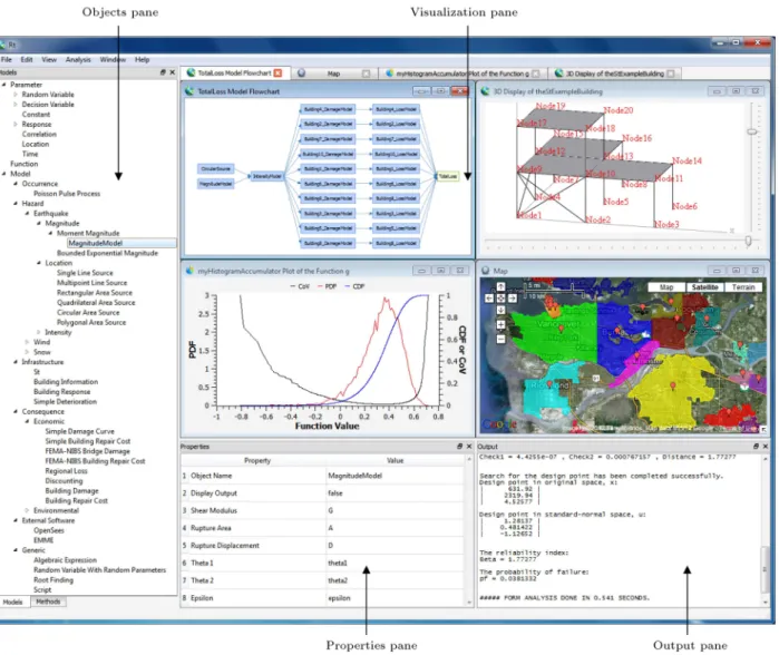
Figure 1 shows the user-interface of Rt. This graphical user interface is designed to promote the proposed multi-model reliability analysis in academia as well as in engineering practice. Dierent panes of Rt's user interface are indicated with arrows in Figure 1. The Objects Pane views and manages all objects, which include parameters, functions, models, and analysis algorithms. The user may instantiate new objects through this pane. The Properties Pane
views and edits the properties of the object that is selected in the Objects Pane. For instance, the user may set the mean and standard deviation of a random variable object through this pane. The Output Pane displays the text output of the analysis, including results and possible errors. Finally, the Visualization Pane demonstrates the graphical output of Rt. Four instances of such outputs are shown in Figure 1. They include a owchart of the models that are employed in the risk analysis on top-left, an OpenGL view of the nite element model of a building under consideration on top-right, a diagram that shows the results of a \histogram sampling" analysis on bottom-left, and a Google Maps® view of the region under consideration
in a risk analysis on bottom-right.
Rt has a growing library of probabilistic models. A part of this library is seen in the Objects Pane of Rt under the branch \Model" in Figure 1. Models are implemented for the occurrence, magnitude, location, and intensity of hazards, performance of structures and infrastructure, and the ensuing consequences, such as economic, socioeconomic, and environmental conse-quences. The user can also implement new models | without any recompilation of the program { by several means, including a scripting option. Furthermore, Rt interfaces with several external computer programs, which include OpenSees [24], ANSYS [25], Abaqus [26], SAP2000 [27], USFOS [28], and EMME [29]. The rst four are sophisticated nite-element analysis programs. USFOS is an oshore structural analysis program and EMME is a transportation network analysis program. In an Rt analysis, each of these programs may serve as a model amongst many other probabilistic models. Further information on Rt is available in [30].
4. Models
A library of probabilistic models is developed for pre-diction of seismic risk. It is specically intended for use with reliability methods to compute event probabilities, such as seismic loss probabilities. Models are proposed for earthquake location and magnitude, building re-sponse, building structural and non-structural damage, building repair cost, and building retrot cost. These models are implemented in Rt. Several other models are available in Rt, while the scope of the analyses in this paper is limited to models pertaining to regional seismic risk.
Several modeling techniques are available to de-velop probabilistic models suitable for reliability anal-ysis. One approach is the development of linear models by Bayesian inference, as described by Box and Tiao [31]. Gardoni et al. [32] applied this approach to reinforced concrete members in the context of seismic risk. This approach is appealing because the resulting models meet the conditions required for use in a
relia-Figure 1. User interface of Rt.
bility analysis. In fact, model uncertainty is explicitly included by means of random model parameters. Each of the following sections presents one of the proposed models.
4.1. Earthquake location model
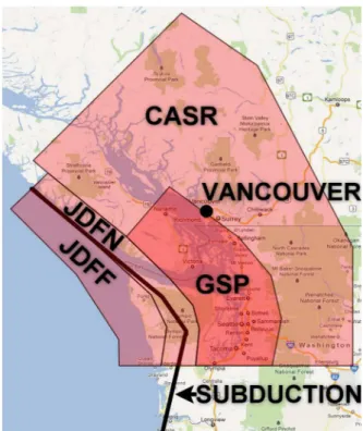
It is usual in the literature to compute the probability distribution of the distance between the earthquake location and the site of interest, R [33]. In contrast, the new location models in Rt model the random rupture location of a seismic event. The models take random variables as input and output a realization of the lati-tude, longilati-tude, and depth of the rupture location [3]. Once the rupture location is known, the distance to any building site is readily computed. Using these models, the sources of seismicity that aect the UBC campus are modeled. The geometry of seismic sources is obtained from Adams and Halchuk [34], and shown in Figure 2 in reference to the City of Vancouver. Five sources of seismicity aect this region. CASR (Cas-cade Mountains, regional), JDFF (Juan de Fuca plate
bending, oshore), and JDFN (Juan de Fuca plate bending, onshore) are area sources for shallow crustal earthquakes, GSP (Georgia Strait/Puget Sound) is an area source for deep subcrustal earthquakes, and the Cascadia fault is modeled as a line source capable of producing megathrust subduction earthquakes. 4.2. Earthquake magnitude model
The magnitude of earthquakes is commonly repre-sented by a bounded exponential random variable [35]. The probability distribution of this random variable is based on the Gutenberg-Richter law [36] and the probability density function is:
f(m) = 1 exp [ bb0 exp [ b0 (M0 (m Mmin)]
max Mmin)] for
Mmin m Mmax; (1)
where m is moment magnitude, b0 the parameter that
depends on the relative occurrence of dierent magni-tudes, Mmin magnitude lower bound taken as 5.0 in
Figure 2. Seismic sources that aect the UBC campus, visualized in Rt's Google Maps®interface.
this paper, and Mmax magnitude upper bound. In this
study, m is modeled as a random variable with random parameters. In particular, the parameters of the distribution of m, namely b0 and M
max, are uncertain
and modeled as lognormal random variables. Such a model employs the concept of \probability transforma-tion", as described by Mahsuli and Haukaas [3], and is implemented in Rt. The mean and standard deviation of b0 and Mmax are computed using their lower, best,
and upper estimates from Adams and Halchuk [34] together with their weights. The resulting properties of these random variables were presented by Mahsuli and Haukaas in [37].
4.3. Ground shaking intensity model
The regional analysis in this study employs models that produce a scalar intensity measure. Specically, models are adopted that take earthquake location and magnitude as input and return the elastic 5%-damped spectral acceleration, Sa, for given periods, Tn, and shear wave velocities, VS30, at specic sites.
For the CASR, JDFN, and JDFF crustal sources, the ground motion prediction equation by Boore and Atkinson [38] is employed. For the GSP subcrustal source, the intra-slab equation from Atkinson and Boore [39] is employed. For subduction earthquakes, the relationship for interface events proposed by Atkin-son and Boore [39] is adopted. All these models are \smoothed" for this study [3] to be utilized in gradient-based reliability analyses, such as FORM. In addition, VS30is modeled as a random variable using a
comprehensive database of VS30-measurements for the
City of Vancouver. Although the numerical example in this paper considers only one intensity model for each seismic source, the analysis framework and the computer program are capable of employing multiple ground motion prediction equations to account for the model uncertainty in predicting the earthquake inten-sity. In this case, the intensities predicted by dierent equations are combined by user-dened weights similar to the well-known \logic tree" method.
4.4. Building response model
Building response models make probabilistic predic-tions of the peak drift ratio, p, and peak
acceler-ation response, Ap. These responses are deemed to
govern the structural and non-structural damage [9]. The information that is input to the building models presented in this paper is gathered by visual inspection, satellite imagery, and municipal databases. The infor-mation includes the building material; load bearing sys-tem; occupancy; year of construction; state of retrot; number of stories; footprint area; plan irregularity, IP I;
vertical irregularity, IV I; soft story, ISS; short column,
ISC; and pounding, IP.
Response models are developed for 13 building types that are identied by the construction material and load bearing system, as described by Mahsuli and Haukaas [3]. The capacity spectrum method [40] described in FEMA-NIBS [9] is employed to generate data for the Bayesian regression analysis. The rst attempt was to model p and Ap in terms of
observ-able building properties, but it provided a poor t. Therefore, a stronger emphasis on structural dynamics was introduced and the following parameters were considered in the model: natural period of vibration, Tn; strength-to-weight ratio, V ; yield drift ratio, y;
ductility capacity, ; ultimate drift ratio, u; and
degradation factor, . Sub-models are established for these parameters separately for each of the 13 types. In turn, the six parameters Tn, V , y, , u, and
are utilized as regressors to model p and Ap for all
building types. A number of dierent model forms were tried. Each model was assessed by plotting the model predictions against the data and the model residuals against the regressors. In this process, some model forms exhibited inadequate predictions and some suered from heteroscedasticity. In conclusion, the models that best predict p and Ap are:
ln(p) = 1+ 2ln(y) + 3ln(u) 4ln (V (1 + v))
5ln() + 6ln(Sa) + 7Sa + "; (2)
ln(Ap) = 1 2ln(y) + 3ln(V ) 4ln()
where i are model parameters and " model errors.
The second-moment information for the model param-eters is obtained from a linear regression analysis and presented by Mahsuli [41]. The models in Eqs. (2) and (3) originally included damping and overstrength as regressors, but they were omitted in a stepwise modeling process as described by Gardoni et al. [32]. The parameter v in the response model is a decision variable that indicates the amount of increase in the lateral strength of the building as a result of seismic retrot. This parameter will later be employed to prioritize buildings in a portfolio for retrot actions. 4.5. Building damage model
Given the responses p and Ap, this section addresses
the ensuing damage. Damage is here expressed as the ratio of the repair cost to the replacement cost of the building. Four damage ratios are developed: 1. Structural damage, S; 2. Non-structural
drift-sensitive damage, ND; 3. Non-structural
acceleration-sensitive damage, NA; and 4. Content damage, C.
The rst two factors depend on p, while the last
two depend on Ap. Data for the regression analysis
is generated using the fragility curves from FEMA-NIBS [9]. To account for the increased damage due to building irregularities, the building scoring system of ATC-21 [42] is employed.
For all models, a smooth increase in damage from 0 to 1 due to increasing building responses is sought. Therefore, polynomial, trigonometric, and logit functions were tested, but the standard normal cumulative distribution function, , turned out to provide the best t. The building irregularities are included in the structural damage model by means of an exponential function. This function produces a factor to increase the damage if irregularities exist. It yields the following model for structural damage:
s=
1+ 2ln(p) + 3ln(H) 4
exp
5IV I+6IP I+7ISS+8ISC+9IP
+";
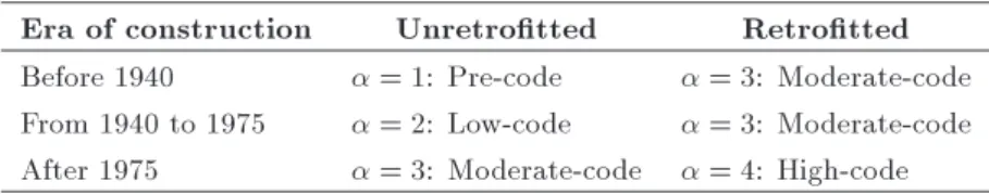
(4) where represents the construction quality and is determined from the year of construction and state of retrot of the building in accordance with Table 1. In particular, = 1 for buildings that are built prior to seismic standards, = 2 for low code, = 3
for moderate code, and = 4 for the building built with high seismic standards. The second-moment information for the model parameters, i, for each
of the 13 building types is presented by Mahsuli [41] and implemented in Rt. The other damage models are considered independent from the building type and irregularities:
ND = (1+ 2ln(p)) + "; (5)
NA= (1ln(Ap) 2) + "; (6)
C = (1ln(Ap) 2) + ": (7)
The negative sign of the iparameters associated with
in Eqs. (4), (6), and (7) correctly indicates that the damage decreases as the quality of construction increases. The model in Eq. (4) suggests that taller buildings incur more damage at the same level of drift ratio. Furthermore, amongst the i parameters that
correspond to irregularities, i.e. 5 to 9 in Eq. (4),
regression yields the highest mean for 7 for most
building types. This implies that soft-story irregularity is the most detrimental type of irregularity. Conversely, 9 has the lowest mean for most building types, which
indicates that pounding imposes the least damage compared with other irregularities.
4.6. Building repair cost model
Provided a damage ratio, the associated repair cost is computed by multiplying it with the building replace-ment cost per unit oor area and the building oor area. Summation of structural, non-structural, and content yields:
cr=
sCs+NDCND+NACNA+CCC
A ";(8) where i are damage ratios from the previous section,
Ci the corresponding replacement costs per unit oor
area which depend on the building occupancy, A the total oor area determined from the number of stories and the footprint area, and " model error which is a normal random variable with unit mean and 10% coecient of variation.
4.7. Building retrot cost model
The model that predicts incremental construction cost associated with retrot is:
co= v(Cs A)
7
4
"o; (9)
Table 1. Building code levels.
Era of construction Unretrotted Retrotted Before 1940 = 1: Pre-code = 3: Moderate-code From 1940 to 1975 = 2: Low-code = 3: Moderate-code After 1975 = 3: Moderate-code = 4: High-code
Figure 3. Map of the UBC campus and the 622 buildings that are modeled in this study.
where represents ratio of the cost of the lateral force-resisting system to the total structural cost, CS
structural cost per unit oor area, A total oor area, code-level factor that expresses the strength of the building prior to retrot, and "o model error factor. In
Eq. (9), the term (7 )=4 implies that the buildings built with high standards cost 25% less to retrot than the moderate code level, while pre-code buildings cost 50% more to retrot than the moderate code level.
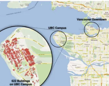
Each of the 622 buildings on the UBC campus are modeled with a building response model, a building damage model, a building repair cost model, and a building retrot cost model. Figure 3 pinpoints this region in the Google Maps® interface in Rt. The
markers in the zoomed map of the UBC campus identify the 622 considered buildings.
5. Methods
The essence of a reliability analysis is random variables collected in the vector x, and limit-state functions, gi(x). Both physical variables, such as magnitude, and
model variables, such as model error, are included in x. The subscript i in gi denotes the ith hazard. That is,
for each hazard, a limit-state function is formulated in the presented methodology. This fosters a multi-hazard risk analysis framework. The primary objective of a reliability analysis with one limit-state function is to determine the probability that the limit-state function will take on negative outcomes. This probability is denoted by pi = P [gi(x) 0]. In other words, the
limit-state function identies the event for which the probability is sought. The limit-state function:
gi(x) = ct ci(x); (10)
is central in this study because it yields the probability that the total cost when the ith hazard occurs, ci(x),
is greater than the threshold, ct. Two costs are
considered: (1) Cost of repair due to earthquake-induced damage, cr; and (2) Cost of construction due
to a priori retrot actions, co. It is emphasized that
the evaluation of ci(x) requires a host of probabilistic
models of the type presented in the previous section. Any reliability method evaluates gi and perhaps
the gradient vector @gi=@x several times, for dierent
realizations of x, to obtain an estimate of pi. The
FORM analysis is an appealing method because it requires only a handful of evaluations of giand @gi=@x
to yield an estimate. FORM also provides valuable insight into the relative importance of each random variable. As described by Der Kiureghian [1], FORM includes a search for the \design point," which is the most likely realization of x associated with gi = 0 in
the space of standard normal variables. The result of the search is the reliability index i, which is related
to the sought probability by the equation:
pi= ( i): (11)
FORM produces a good estimate of pi depending on
the topology of the limit-state surface near the design point. This result may be inaccurate if the limit-state function is strongly nonlinear in the space of standard normal variables. Under such circumstances, the SORM and importance sampling are utilized to improve the FORM result; see details in [1-20].
The problem under consideration has several limit-state functions of the form of Eq. (10) because several sources of seismic hazard are present. Speci-cally, the region is subjected to crustal, subcrustal, and subduction earthquakes, as described before. Because each of these sources is associated with dierent loca-tion and magnitude models, they are modeled as dier-ent hazards with dierdier-ent occurrence rates. As a result, multi-hazard analysis is necessary when analyzing the seismic risk for the UBC campus. Two multi-hazard analysis methods are available in Rt. One that is employed here is based on the load coincidence method described by Wen [23]. It was originally proposed for load combination and in this paper, it is extended to loss analysis applications. It employs the Poisson pulse process and accounts for the possible coincidence of two or more hazards. However, the formulation is simplied in the seismic-oriented case study in this paper because the probability of the coincidence of two earthquakes is negligible. This implies that the Poisson point process is employed to model the hazards, each with a rate of occurrence denoted by i; i = 1; 2; 3; :::; N, where N is
the total number of hazards.
Suppose a reliability analysis is carried out for each hazard, so that iand piare known for all hazards.
Consequently, the rate of exceeding the cost threshold ct is ipi for each hazard. The combined rate that
includes all hazards is the sum of the individual rates, and the well-known Poisson distribution provides the probability of exceedance within a time period, T :
p = 1 exp T
N
X
i=1
ipi
!
; (12)
where p is the probability that the total cost, c(x), exceeds the threshold, ct, when all hazards are
consid-ered. In the context of FORM analysis, it is common to employ a generalized reliability index, , as a surrogate measure for p:
= 1(p); (13)
where 1 represents standard normal inverse
cumu-lative distribution function.
A risk analysis is carried out to obtain the probability distribution of the total seismic costs for the UBC campus. This analysis includes 4389 model instances, 8097 model responses, and 281 random variables. The analysis is conducted for the current state of the buildings, i.e. v = 0 for all buildings. Figure 4 shows the cost exceedance probability curve for a time span of 50 years, i.e. T = 50. It is noted that the exceedance probabilities diminish rapidly as the cost threshold increases. For example, the probability of exceeding $100M is 0.0365, while the probability of exceeding $500M is 0.0071.
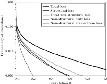
To get further insight from this analysis, the con-tribution of structural and non-structural components of the UBC buildings to overall losses is illustrated in Figure 5. A logarithmic scale is employed to highlight the tail probabilities. Figure 5 shows that the probability of exceedance for non-structural losses, i.e. the sum of acceleration- and drift-sensitive losses, is higher than that of structural losses. This has been observed in several studies, see e.g. FEMA-NIBS [9].
Figure 4. Cost exceedance probability curve.
Figure 5. Structural and non-structural loss probabilities.
Figure 6. Damage ratio probabilities for dierent building types.
In turn, non-structural drift-sensitive components con-tribute more to the loss probabilities than acceleration-sensitive components.
Next, the performance of dierent structural sys-tems and construction materials is assessed to deter-mine the relative vulnerability of dierent building types. For this purpose, a \prototype damage ratio" is dened. For each building type, it equals the total loss of all buildings with that type divided by their total value. Figure 6 presents the probability of exceeding damage ratios for T = 50 years for dierent building types. This gure indicates that unreinforced masonry buildings are the most vulnerable, while concrete shear wall buildings are the least. Note that this ranking is specic to the composition of buildings at UBC. For example, most of the modern concrete buildings at UBC are shear wall buildings, which exhibit the best performance according to Figure 6.
6. Sensitivity measures
Suppose the manager of a building portfolio seeks to allocate limited resources in an optimal manner to
retrot selected buildings. One approach is to establish a decision tree that compares the cost of retrot with the expected cost of damage for each building. However, the risk analysis presented earlier yields the entire distribution of cost. Hence, an approach that goes beyond expected cost is desirable. To this end, the sensitivity measure, @=@co, is proposed and discussed
in this section, where co is cost spent on retrot. The
fundamental idea behind @=@cois that buildings that
yield the largest increase in the reliability index, i.e., the largest reduction in cost exceedance probability, per dollar spent on retrot should be prioritized. To evaluate @=@co, it is necessary to recognize that
depends on co through p, pi, i, and v. The chain rule
of dierentiation yields: @
@co =
@ @p
N
X
i=1
@p @pi
@pi
@i
@i
@v @v @co
: (14)
For convenience of subsequent derivations, the rst three derivatives in the right-hand side are merged and evaluated by dierentiation of Eqs. (11)-(13), which yields:
@ @i =
@ @p
@p @pi
@pi
@i =
1 '()T i
exp
T XN
i=1
ipi
'(i); (15)
where ' is standard normal probability density func-tion. According to Eq. (15), the value of @=@i
increases with the occurrence rate, i, and decreases
with the reliability index, i. In other words, frequent
and/or damaging hazards contribute more to the sen-sitivity in Eq. (14). The derivative @i=@v in the
right-hand side of Eq. (14) is obtained by dierentiating the reliability index from FORM [1]:
@i
@v = 1 jjrGijj
@gi
@v
x; (16)
where Gi stands for limit-state function in the space
of standard normal variables, and the asterisk denotes the realization of random variable at the design point. Eq. (16) requires the derivative of gi in Eq. (10), which
in turn requires the derivative of the models that enter into the evaluation of total cost. These derivatives are available in Rt because each model computes response sensitivities by the direct dierentiation method [2]. The last derivative in the right-hand side of Eq. (14) represents the marginal cost of retrot; dierentiation of Eq. (9) yields:
@co
@v = (CSA)
7 4
"o: (17)
To prioritize the buildings on the UBC campus for seismic retrot, the sensitivity measure @=@co in
Eq. (14) is computed for each of the 622 buildings at their present state, i.e. v = 0. For this purpose, the cost threshold, ct, in Eq. (10), is set to $100 million. This
means that the reliability index in Eq. (14) corresponds to the probability that the maximum seismic cost in this region exceed $100 million over the next 50 years. Table 2 displays the value of @=@co for the 10
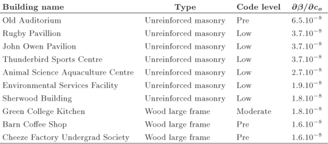
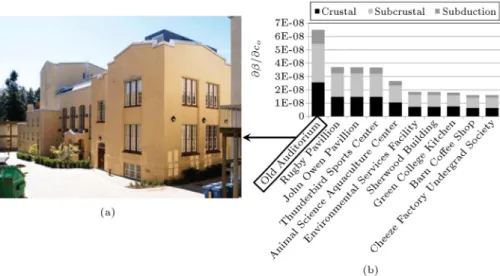
highest ranked buildings. It is observed that most of the highest ranked buildings are unreinforced masonry structures. This is not surprising, because unreinforced masonry buildings tend to sustain signicant damage in earthquakes. It is also observed in Table 2 that most of the highest ranked buildings belong to pre-code and low-code levels. In other words, they are either built before seismic codes appeared around 1940 or before the seismic codes were upgraded around 1975. For example, the \Old Auditorium", which ranks at the top in Table 2 and is shown in Figure 7(a), is a large unreinforced masonry structure built in 1925. The value of @=@cofor this building implies that spending
$154,000 on retrot changes the reliability index for the entire campus by 0.01. This is more than any other building on the UBC campus.
Table 2. Top 10 buildings according to retrot priority.
Building name Type Code level @=@co
Old Auditorium Unreinforced masonry Pre 6:5:10 8
Rugby Pavillion Unreinforced masonry Low 3:7:10 8
John Owen Pavilion Unreinforced masonry Low 3:7:10 8 Thunderbird Sports Centre Unreinforced masonry Low 3:7:10 8 Animal Science Aquaculture Centre Unreinforced masonry Low 2:7:10 8 Environmental Services Facility Unreinforced masonry Low 1:9:10 8 Sherwood Building Unreinforced masonry Low 1:8:10 8 Green College Kitchen Wood large frame Moderate 1:8:10 8
Barn Coee Shop Wood large frame Pre 1:6:10 8
Figure 7. (a) Old auditorium. (b) Top 10 buildings according to retrot priority.
The diagram in Figure 7(b) disaggregates @=@co
to expose the contributions of crustal, subcrustal, and subduction earthquakes. The gure indicates that the highest contribution to the cost sensitivities is of crustal earthquakes. This is reasonable because sub-crustal earthquakes are associated with relatively high frequency and high probabilities of cost exceedance.
The positive value of @=@co in Table 2 suggests
that it is worthwhile to allocate resources to retrot these buildings. In fact, positive values of @=@co are
observed for 393 buildings on campus, which is about 63% of the building stock. Conversely, @=@co takes
on negative values for the other 229 buildings. The negative sign indicates that it is not worthwhile to retrot these 229 buildings because the construction cost surpasses the gain from decreased damage. Table 3 shows the negative values of @=@co for the 10 lowest
ranked buildings. These buildings yield the largest increase in cost exceedance probability per dollar spent on retrot. It is observed that Table 3 contains mostly concrete shear wall buildings. This is not surprising, because the lateral force-resisting system of
these buildings is specically designed to carry high seismic forces. In fact, the buildings in Table 3 belong to the moderate-code level, which means that they are built after 1975 or retrotted to contemporary codes. It is therefore reasonable that these buildings are not prioritized for seismic retrot according to the measure @=@co.
It is noted, however, that these sensitivity mea-sures only consider economic losses due to structural and non-structural repair costs, and do not account for social losses due to injury and death. Probabilistic models for predicting social losses are being developed in ongoing research by the author. The lack of such models in the numerical example here is remedied by selecting a \risk-averse" measure of risk. A neutral measure of risk would be the mean regional loss. However, in lieu of computing the sensitivities at the mean regional loss, i.e. $16M, they are computed at a quantile in the upper tail of the loss probability distribution, i.e. $100M. As a result, @=@cois positive
for a larger number of buildings. In other words, the sensitivity measure that is computed in the tail of the
Table 3. Bottom 10 buildings according to retrot priority.
Building name Type Code level @=@co
Animal Care Rodent Breeding Concrete shear wall Moderate 2:1:10 9 Animal Science Main Sheep Unit Concrete moment frame Moderate 1:8:10 9 Acadia Park Highrise Concrete shear wall Moderate 1:7:10 9
The Regency Concrete shear wall Moderate 1:6:10 9
ChemBio Engineering Concrete shear wall Moderate 1:6:10 9
The Chatham Concrete shear wall Moderate 1:6:10 9
Irving Barber Library Concrete shear wall Moderate 1:6:10 9 Technology Enterprise Facility Concrete shear wall Moderate 1:6:10 9
ICICS Main Concrete shear wall Moderate 1:6:10 9
loss distribution indicates a larger number of buildings in need of seismic retrot than a sensitivity measure computed at the mean loss.
It is observed that unreinforced masonry buildings are the top candidates for retrotting, while those that are not worthwhile to retrot are mostly concrete shear wall buildings. This rearms the ndings in Figure 6. This gure shows that concrete shear wall buildings at UBC exhibit the best seismic performance, while unreinforced masonry buildings exhibit the poorest.
7. Conclusion remarks
This paper revisits risk analysis and risk-based decision making in structural and earthquake engineering. The methodology for risk analysis in the present study contrasts the approaches in the literature in two as-pects: treatment of uncertainties, and computation of risk. In the existing approaches, the uncertainty is described by conditional probability models, e.g. fragility curves that output a probability conditioned upon the value of input(s). Thereafter, risk is typically computed in either of these two ways: 1) Computing the expectation of the loss; 2) Integrating the condi-tional probabilities by the theorem of total probability to compute the probability that the loss exceeds a threshold. In contrast, the uncertainty in the present approach is described by random variables that are input to models. Given the realization of these random variables, the model produces a physical measureable output, such as spectral acceleration and seismic loss, not a probability. In turn, risk, i.e. the probability of exceeding a loss threshold, is computed by reliability methods. This reliability-based approach oers the following advantages:
1. Uncertainties are explicitly characterized by ran-dom variables. In contrast, uncertainties are im-plicit in conditional probability models;
2. By-products of the reliability analysis, i.e. im-portance and sensitivity measures, are employed for optimal risk mitigation, which maximize the resilience of infrastructure;
3. Many of the existing engineering models that re-ceive a number of inputs and produce physical output(s) can be employed in the analysis, provided that the uncertainty in the model is properly characterized by random variables. For instance, nite element models can be directly incorporated in the analysis;
4. Risk is computed when multiple hazards are present, and the possible coincidence of hazards is accounted for;
5. The models can take limitless number of inputs and provide limitless number of outputs to many
downstream models. The limit is determined by the memory of the computer. In contrast, the conditional probability models are typically limited to one or two inputs and provide a single output;
6. Portfolio level analyses are readily carried out by modifying the limit-state function to include the sum of the losses of multiple structures and infras-tructure, e.g. all buildings in a region;
7. The probabilities are computed by ecient reliabil-ity methods, rather than a multifold integral, which may be cumbersome to evaluate;
8. It is possible to include time-varying phenomena, such as long-term deterioration and discounting, in the analysis; see Mahsuli and Haukaas [30,37] for numerical examples;
9. It is possible to distinguish between reducible and irreducible uncertainties, which are termed epis-temic and aleatory uncertainties, respectively. This permits targeted eorts to reduce the epistemic uncertainty.
Acknowledgment
The nancial support from Sharif University of Tech-nology through the Grant Number G930930 is grate-fully acknowledged. The author thanks Professor Terje Haukaas for his support throughout the course of this research. The author also thanks Mr. Amin Ghasemi for his assistance in word-processing of the bibliography.
References
1. Der Kiureghian, A. \First-and second-order reliability methods", Engineering Design Reliability Handbook, E. Nikolaidis, D.M. Ghiocel, and S. Singhal, Eds., CRC Press, Boca Raton, FL, USA (2005).
2. Kleiber, M., Hien, T.D., Antunez, H. and Kowalczyk, P., Parameter Sensitivity in Nonlinear Mechanics: Theory and Finite Element Computations, Wiley, West Sussex, UK (1997).
3. Mahsuli, M. and Haukaas, T. \Seismic risk analysis with reliability methods, part I: Models", Struct. Saf., 42, pp. 54-62 (2013b).
4. Cornell, C.A. \Engineering seismic risk analysis", Bull. Seismol. Soc. Am., 58(5), pp. 1583-1606 (1968).
5. McGuire, R.K. \Seismic structural response risk anal-ysis incorporating peak response regressions on earth-quake magnitude and distance", Report Publ. 399, Dept. of Civil Eng., Massachusetts Institute of Tech-nology, Boston, MA, USA (1974).
6. McGuire, R.K. and Barnhard, J.A. \Magnitude, dis-tance, and intensity data for C.I.T. strong motion records", Journal of Research of the United States Geological Survey, 5(4), pp. 437-443 (1977).
7. McGuire, R.K. \Probabilistic seismic hazard analysis: Early history", Earthquake Eng. Struc., 37(3), pp. 329-338 (2008).
8. ATC \Earthquake damage evaluation for California", Report ATC-13, Applied Technology Council, Red-wood City, CA, USA (1985).
9. FEMA-NIBS, Earthquake Loss Estimation Methodol-ogy - HAZUS Technical Manual, Federal Emergency Management Agency and National Institute of Build-ing Sciences, WashBuild-ington, DC, USA (2003).
10. Choe, D., Gardoni, P., Rosowsky, D. and Haukaas, T. \Probabilistic capacity models and seismic fragility estimates for RC columns subject to corrosion", Reliab. Eng. Syst. Safe., 93(3), pp. 383-393 (2008).
11. Cornell, C.A. and Krawinkler, H. \Progress and chal-lenges in seismic performance assessment", PEER Center News, Berkeley, CA, USA (2000).
12. Moehle, J. and Deierlein, G.G. \A framework method-ology for performance-based earthquake engineering", 13th World Conference on Earthquake Engineering, Vancouver, BC, Canada, pp. 3812-3814 (2004).
13. Yang, T.Y., Moehle, J., Stojadinovic, B. and Der Kiureghian, A. \Seismic performance evaluation of fa-cilities: Methodology and implementation", J. Struct. Eng., 135(10), pp. 1146-1154 (2009).
14. Ellingwood, B.R. and Wen, Y. \Risk-benet-based design decisions for low-probability/high-consequence earthquake events in Mid-America", Prog. Struct. Eng. Mater., 7(2), pp. 56-70 (2005).
15. Cornell, C.A. \Bounds on reliability of structural systems", J. Struct. Div-ASCE, 93(1), pp. 171-200 (1967).
16. Ditlevsen, O., Structural Reliability and the Invariance Problem, University of Waterloo, Solid Mechanics Division, Canada (1973).
17. Hasofer, A.M. and Lind, N.C. \Exact and invariant second-moment code format", J. Eng. Mech. Div-ASCE, 100(1), pp. 111-121 (1974).
18. Breitung, K. \Asymptotic approximations for multi-normal integrals", J. Eng. Mech., 110(3), pp. 357-366 (1984).
19. Hohenbichler, M. and Rackwitz, R. \Improvement of second-order reliability estimates by importance sampling", J. Eng. Mech., 114(12), pp. 2195-2199 (1988).
20. Ditlevsen, O. and Madsen, H.O., Structural Reliability Methods, John Wiley & Sons, Chichester, UK (1996).
21. Der Kiureghian, A. and Taylor, R.L. \Numerical methods in structural reliability", 4th International Conference on Application of Statistics and Probability in Civil Engineering, Florence, Italy (1983).
22. Koduru, S.D. and Haukaas, T. \Probabilistic seismic loss assessment of a Vancouver high-rise building", J. Struct. Eng., 136(3), pp. 235-245 (2010).
23. Wen, Y.K., Structural Load Modeling and Combina-tion for Performance and Safety EvaluaCombina-tion, Elsevier, Amsterdam, Netherlands (1990).
24. McKenna, F., Fenves, G.L. and Scott, M.H., Open System for Earthquake Engineering Simulation, Pacic Earthquake Engineering Research Center, University of California, Berkeley, CA, USA (2003).
25. ANSYS Inc. \ANSYS 14.0 theory guide", PA, USA (2003).
26. Dassault Systems, \Abaqus 6.13 analysis user's guide", RI, USA (2013).
27. Computers and Structures Inc., \CSI SAP2000", Berkeley, CA, USA (2015).
28. USFOS \USFOS 8.7 user's manual", Bergen, Norway (2014).
29. INRO \EMME 3", Canada (2009).
30. Mahsuli, M. and Haukaas, T. \Computer program for multimodel reliability and optimization analysis", J. Comput. Civ. Eng., 27(1), pp. 87-98 (2013a).
31. Box, G.E.P. and Tiao, G.C., Bayesian Inference in Statistical Analysis, Wiley-Interscience, NJ, USA (1992).
32. Gardoni, P., Der Kiureghian, A. and Mosalam, K.M. \Probabilistic capacity models and fragility estimates for reinforced concrete columns based on experimental observations", J. Eng. Mech., 128(10), pp. 1024-1038 (2002).
33. Der Kiureghian, A. and Ang, A.H. \A fault-rupture model for seismic risk analysis", Bull. Seismol. Soc. Am., 67(4), pp. 1173-1194 (1977).
34. Adams, J. and Halchuk, S. \Fourth generation seismic hazard maps of Canada: Values for over 650 Cana-dian localities for the 2005 National Building Code of Canada", Report Open File 4459, Geol. Surv. of Canada, Ottawa, ON, Canada (2003).
35. McGuire, R.K., Seismic Hazard and Risk Analysis, Earthquake Engineering Research Institute, Berkeley, CA, USA (2004).
36. Gutenberg, B. and Richter, C.F. \Frequency of earth-quakes in California", Bull. Seismol. Soc. Am., 34(4), pp. 185-188 (1944).
37. Mahsuli, M. and Haukaas, T. \Seismic risk analysis with reliability methods, Part II: Analysis", Struct. Saf., 42, pp. 63-74 (2013c).
38. Boore, D.M. and Atkinson, G.M. \Ground-motion prediction equations for the average horizontal compo-nent of PGA, PGV, and 5%-damped PSA at spectral periods between 0.01 s and 10.0 s", Earthq. Spectra, 24(1), pp. 99-138 (2008).
39. Atkinson, G.M. and Boore, D.M. \Empirical ground-motion relations for subduction-zone earthquakes and their application to Cascadia and other regions", Bull. Seismol. Soc. Am., 93(4), pp. 1703-1729 (2003).
40. Mahaney, J.A., Paret, T.F., Kehoe, B.E. and Freeman, S.A. \The capacity spectrum method for evaluating structural response during the Loma Prieta earth-quake", 1993 U.S. Natl. Earth. Conf., Central United States Earthquake Consortium (CUSEC), pp. 501-510 (1993).
41. Mahsuli, M. \Probabilistic models, methods, and software for evaluating risk to civil infrastructure", PhD Dissertation, University of British Columbia, Vancouver, BC, Canada (2012).
42. ATC. \Rapid visual screening of buildings for poten-tial seismic hazards: A handbook", Report ATC-21,
Applied Technology Council, Redwood City, CA, USA (1988).
Biography
Mojtaba Mahsuli is an Assistant Professor in the Department of Civil Engineering at Sharif University of Technology. He received his BS and MS degrees from Sharif University and his PhD degree from the University of British Columbia. Dr. Mahsuli conducts research on evaluation and optimal mitigation of risk to civil infrastructure under multiple hazards.