Accessing and developing the required biophysical datasets and data layers for Marine Protected Areas network planning and wider marine spatial planning purposes Report No. 20, Task 2F.UK marine benthic diversity layer.

(1)

1

Accessing and developing the required biophysical data sets and

data layers for Marine Protected Areas network planning and wider

marine spatial planning purposes

Task 2F - Development of a marine diversity data layer: review of approaches and proposed method

16 September 2009

© Crown copyright

(2)

2

Project Title: Accessing and developing the required biophysical data sets and data layers for Marine Protected Areas network planning and wider marine spatial

planning purposes

Report 2: Task 2F - Development of a marine diversity data layer: review of approaches and proposed method

Project Code: MB0102 Marine Biodiversity R&D Programme Defra Contract Manager: Jo Myers

Funded by:

Department for Environment Food and Rural Affairs (Defra) Marine and Fisheries Science Unit

Marine Directorate Nobel House 17 Smith Square London SW1P 3JR

Joint Nature Conservation Committee (JNCC) Monkstone House

City Road Peterborough PE1 1JY

Countryside Council for Wales (CCW) Maes y Ffynnon

Penrhosgarnedd Bangor

LL57 2DW

Natural England (NE) North Minister House Peterborough

PE1 1UA

Scottish Government (SG)

Marine Nature Conservation and Biodiversity Marine Strategy Division

Room GH-93 Victoria Quay Edinburgh EH6 6QQ

(3)

3

Department of Environment Northern Ireland (DOENI) Room 1306

River House 48 High Street Belfast

BT1 2AW

Isle of Man Government (IOM)

Department of Agriculture Fisheries and Forestry Rose House

51-59 Circular Road Douglas

Isle of Man IM1 1AZ

(4)

(5)

5 Authorship:

E.L. Jackson

MarLIN Biodiversity and Conservation Science Programme Manager [email protected]

O. Langmead

MarLIN Biodiversity and Conservation Science Programme Manager [email protected]

K. Hiscock MarLIN

[email protected] H. Tyler-Walters

MarLIN Strategic Director [email protected]

P. Miller

Plymouth Marine Laboratory [email protected]

A. McQuatters-Gollop

Sir Alister Hardy Foundation for Ocean Science [email protected]

J. Saunders ABPMer

[email protected] C. Fox

Scottish Association for Marine Science [email protected]

The Marine Life Information Network® for Britain and Ireland (MarLIN)

The Marine Biological Association of the United Kingdom PlymouthPL1 2PB

http://www.marlin.ac.uk

This report should be cited as:

Jackson, E.L., Langmead, O., McQuatters-Gollop, A., Miller, P., Fox, C., Hiscock, K., Tyler-Walters, H., Saunders, J., 2009. Development of a marine diversity data layer: review of approaches and proposed method. Report to the Department of

Environment, Food and Rural Affairs from the Marine Life Information Network (MarLIN) Plymouth: Marine Biological Association of the UK subcontracted by ABPMer, Southampton. . Defra Contract No. MB102 Task 2F, Report No. 2.

(6)

6

Disclaimer: The content of this report does not necessarily reflect the views of Defra, nor is Defra liable for the accuracy of information provided, or responsible for any use of the reports content.

Acknowledgements: To Andrew Pearson and Nigel West of ABPmer for the front cover images. The authors would like to thank Prof. John Spicer and Dr. Andy Foggo for their advice on the theory and measurement of “biodiversity”, and to all those who contributed to the biodiversity workshop held to inform this review (see Appendix 1 for a full list of attendees). We also wish to specifically thank Prof. Michel Kaiser, Dr. Jen Ashworth, Beth Stoker and Dr. Kirsten Ramsay for their comments on an earlier draft of the report. Finally, the review section of this report benefitted significantly from the constructive comments of an anonymous independent reviewer.

(7)

7

Executive summary

The UK is committed to the establishment of a network of marine protected areas (MPAs) to conserve marine ecosystems and marine biodiversity. MPAs are a valuable tool to protect rare and threatened species and the integrity and functioning of habitats. They can also be used to aid implementation of the Ecosystem Approach to management, which aims to maintain the ecosystem goods and services produced by the normal functioning of the marine ecosystem that are relied on by humans (Smith & Maltby 2003).

A consortium1 led by ABPmer has been commissioned to develop a deliver a series of biophysical data layers to aid in the selection of a network of Marine Conservation Zones (MCZs) in England and Wales (and the equivalent MPA measure in Scotland) under the Marine and Coastal Access Bill (Contract Reference: MB0102). These data layers will also be of wider use for taking forward marine planning in UK waters. The overall aim of the project is to ensure that the best available information is obtained for the selection of MPAs in UK waters, and that these data layers can be easily accessed and utilised by those who will have responsibility for selecting sites. The project has been divided into a number of tasks, one of which was to review and assess approaches for the development of a „marine biodiversity‟ data layer2. The identification of areas of high marine biodiversity is important to aid the conservation of structurally and functionally important areas, but may also enable the cost effective prioritisation of areas for protection.

This report provides a critical review of approaches to identify areas of high marine biodiversity and how these can be used to inform the selection of MPAs. Biodiversity area is used here to describe areas of species and habitat diversity. The various measures to quantify marine diversity are critically reviewed (e.g. diversity indices, number of species, number of priority species and taxonomic distinctness). The review highlights the limits of data quality and coverage and considers techniques for effort standardisation and validation (assigning confidence) that are fundamental for interpretation of variable data. Particularly in the pelagic and offshore benthic environments appropriate data are so limited that proxy indicators of diversity are required, since data for directly assessing diversity do not exist. We also review past uses of the term biodiversity hotspots and explore issues involved with employing this approach to UK waters.

Based on the conclusions of the review, it is recommended that no single layer adequately represents marine biodiversity and it is proposed that a series of layers are developed. These are presented according to data availability, suitability to represent overall biodiversity and conservation management constraints, and cost effectiveness.

1

ABPmer, MarLIN, Cefas, EMU Limited, Proudman Oceanographic Laboratory (POL) and Bangor University

2

The layer was originally to be called Biodiversity hotspot layer, however, because the it will be presented as a continuous scale of diversity, without predefined levels of what is diverse the layer has been renamed a „marine diversity data layer‟.

(8)

8

For the UK benthos, the most appropriate (suitable for variable data sets) and comprehensive measures (encompassing diversity at different organisational levels) are species and habitat richness, taxonomic distinctness and habitat distinctness. Species and habitat richness are the most commonly recorded units of diversity and do not require abundance data, which can add a significant bias when handling data from multiple sources. Similarly taxonomic distinctness can be calculated without abundance data and provides additional information on the phylogenetic diversity of a site which is arguably more meaningful in terms of maintaining ecosystem function. Biodiversity assessment is arguably less developed in the pelagic realm; it presents different challenges to the benthos due its inherent mobility and variability over a range of spatial and temporal scales, and because data to directly assess diversity are scarce. A series of metrics spanning different levels of ecological organisation were examined encompassing direct measures of diversity for different ecosystem components, satellite earth observation surrogate measures and indicators such as pelagic megafauna. It was concluded that many of the measures previously advocated as indicators of pelagic diversity (e.g. productivity or single species distributions) have insufficient scientific evidence supporting their relationship with overall pelagic diversity at the scale under consideration. Thermal fronts data however, has good spatial coverage and has been correlated with pelagic top predator diversity (a large scale indicator of pelagic biodiversity) and is recommended as an appropriate surrogate.

We propose an approach for future work to assess the marine biodiversity of UK waters that considers the pelagic and benthic realms separately (as they are reviewed here), but entails a common set of steps (although individual data layers will require separate methodologies):

1. examining and collating the available data; 2. data quality assessment and filtering; 3. selection of appropriate spatial scale; 4. analysing the data;

5. standardising for sampling effort (Monte Carlo techniques and regression if appropriate); and

6. validation and confidence assessment.

For the benthos separate analyses for the intertidal and subtidal inshore are proposed at different grid scales. For these regions, the assessment will focus on all macrobenthic species (but excluding fish) and habitats data, and will utilise actual records of species and habitats (including data collated as part of tasks 2B and 2C). Data will be grouped into broad collection methodology following quality assessment and filtering, before calculating the diversity metrics and carrying out other standardisation techniques.

For the pelagic biodiversity surrogate data layer, the proposed approach is to exploit a long term time series of EO SST data to map persistently occurring thermal fronts in UK waters. Initially, monthly maps at 1km resolution would be generated, and the second stage would be to aggregate these into seasonal front climatologies to identify strong, persistent and frequently occurring features, which would be presented along with their confidence.

(9)

9

Appendices

Appendix 1 Biodiversity Hotspots Workshop Transcript by Justine Saunders, ABPMer ... 63 Appendix 2 Proposed approaches for non priority measures/ indicators for the Benthic diversity data

layers ... 75 Appendix 3 Proposed approaches for non priority measures/ indicators for the Pelagic diversity data

(11)

11

List of Figures

Figure 1 Hypothesized mechanisms linking biodiversity and ecosystem functioning (Source: Loreau et al. 2001) ... 16 Figure 2 species accumulation curve showing relationship between the species richness and

sampling effort. ... 29 Figure 3 Tree diagram showing the proposed division of the UK territorial seas for the purpose of

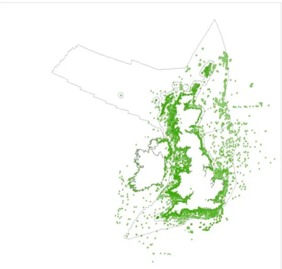
producing the diversity area data layers... 42 Figure 4 Locations of marine survey data collated (at the time of production of the current report) to

support the production of the Biodiversity data layer. Grey lines illustrate UK marine

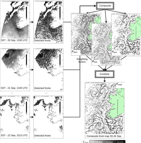
administrative regions. ... 43 Figure 5 Schematic diagram of composite front map technique. 30 AVHRR SST maps (three shown)

of the Irish shelf within a 7-day window are processed to detect front locations, which are then composited to calculate the mean frontal gradient Fmean, the probability of detecting a front Pfront, and the evidence for a feature in proximity Fprox. These weighting factors are combined as the composite front map Fcomp to provide optimal visualisation of all oceanic features observed during the period. ... 49 Figure 6 Front aggregation method. (a) Each grid location is analysed through the time-series of

monthly fronts to calculate the percentage of months in which a strong front was observed. (b) Example front climatology map for June for UK SW area using 2003-2007 data. ... 50 Figure 7 Spatial variation in Hill‟s N1 (exponential Shannon Weiner) and Hill‟s N2 (reciprocal Shannon Weiner) across the North Sea based on the ICES International Bottom Trawl Survey using GOV TV3 trawl (IBTS GOV) data set, illustrating the effect of taking into account species- and size-related catchability in the GOV trawl data (Fraser et al. 2008). ... 76 Figure 8 CPR samples collected in the North Atlantic since 1948. ... 79 Figure 9 Distribution of herring in the North Sea from the IBTS GOV trawl survey. ... 81 Figure 10 Biomass of mature (left panel) and immature (right panel) herring in the North Sea in 2006

from the combined acoustic cruises (source:(Herring Assessment Working Group for the Area South of 62° N 2007b). ... 81 Figure 11 Irish Sea herring VIIa(N). (A) Density distribution of 1-ring and older herring (size of ellipses

is proportional to square root of the fish density (t n.mile-2) per 15-minute interval). Maximum density was 1100 t n.mile-2. (B) Density distribution of 0-ring herring. Maximum density was 100 t n.mile-2. Note: same scaling of ellipse sizes on above figures (source: Herring Assessment Working Group for the Area South of 62° (2007a). ... 82 Figure 12 Puffin distribution in North-East Atlantic waters. ... 85 Figure 13 Distribution of sightings of harbour porpoise (Phocoena phocoena). Source: North-West

European waters for a Cetacean Atlas (Reid et al. 2003). ... 86 Figure 14 Mean Monthly Standardised Sightings Rates of Harbour porpoises (1980-2002). (Source:

Evans & Wang 2008) ... 87 Figure 15 Illustration of improvement to chlorophyll-a estimation in turbid shelf-seas using OC5

algorithm. Aqua-MODIS 7-day chlorophyll-a maps for UK southwest region on 12 June 2008: (a) standard NASA OC3 algorithm; (b) turbid water OC5 algorithm with rings indicating areas where errors due to suspended sediment were significantly reduced. ... 88 Figure 16 Distributions of basking sharks determined using the three methods of (a) tag geolocations

(2001–2003), (b) survey sightings (1994–2003) and (c) public sightings (1987–May 2004) (Source: Southall et al. 2005). ... 90 Figure 17 Contour plots showing (a) the total number of basking sharks sighted per 0.5 x 0.5o

(latitude/longitude) grid cell and (b) total amount of time (h) searched per grid cell (Source: Southall et al. 2005)... 91

(12)

12

List of Tables

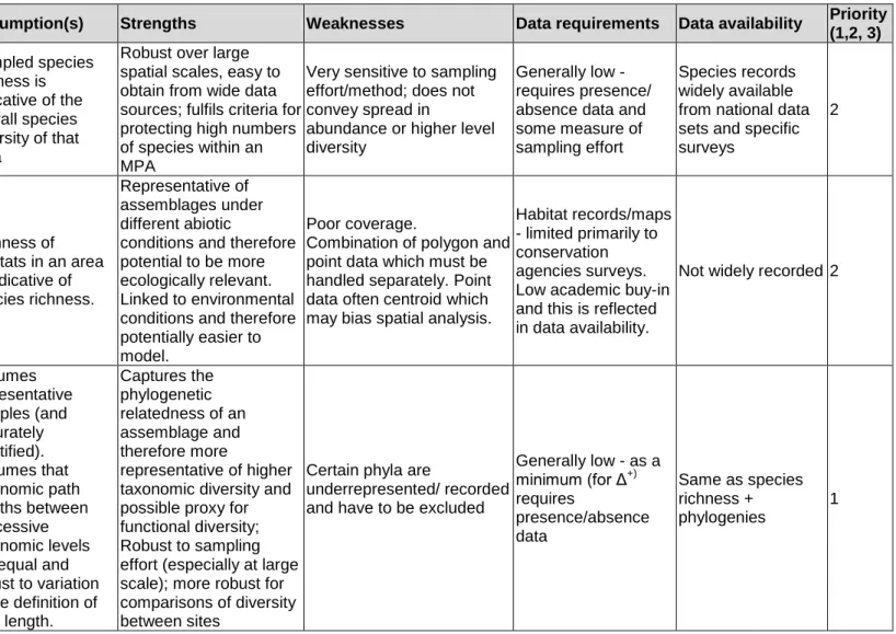
Table 1. Multi-species measures that have been proposed as surrogates for the biodiversity of the total species pool ... 18 Table 2 Examples of the measures used to identify areas of biodiversity ... 20 Table 3 Summary of proposed measures for the production of a biodiversity data layer and

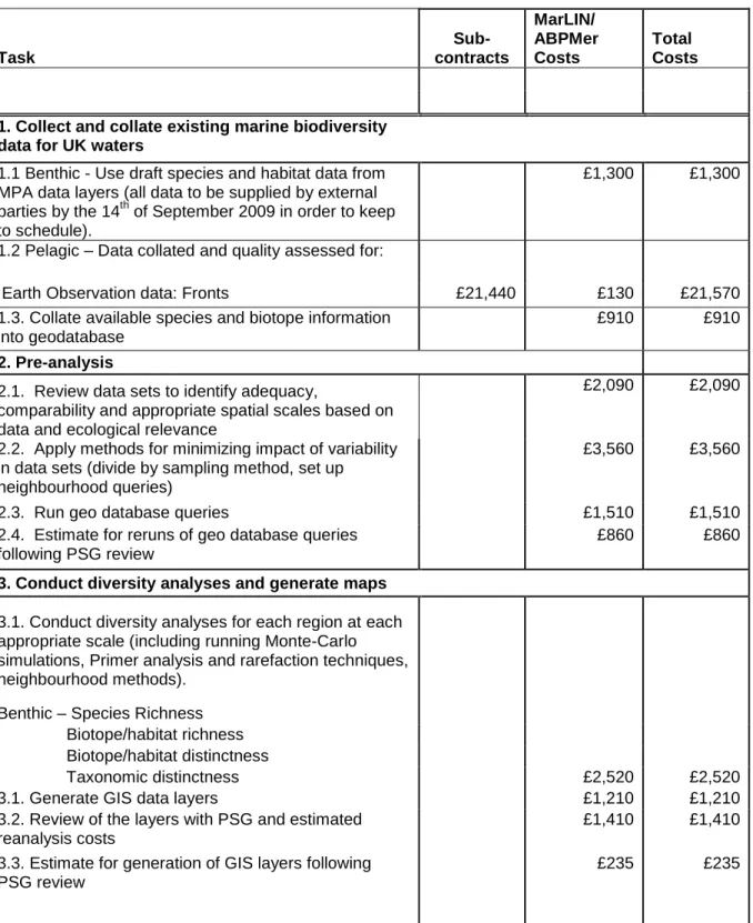
prioritisation ... 37 Table 4. Costs for carrying out Task 2F Biodiversity areas layers. Deliver all layers by 29th January

2010 ... 51 Table 5 Indicative timetable for carrying out Task 2F Biodiversity areas layers: Deliver draft 29th

(13)

13

Introduction

1.1 Biophysical Data layers Project

1.1 The UK is committed through international agreements and European obligations to the establishment of a network of Marine Protected Areas (MPAs) to conserve marine ecosystems and marine biodiversity. The UK Government has also made a commitment under the Marine and Coastal Access Bill to take forward a network of Marine Conservation Zones (MCZs) to conserve and promote the recovery of a wide range of habitats and species. The Scottish Government is also considering equivalent provisions for its waters out to 200nm.

1.2 A consortium3 led by ABPmer has been commissioned to develop a deliver a series of biophysical data layers to aid in the selection of a network of Marine Conservation Zone (MCZ) in England and Wales (and the equivalent MPA measure in Scotland) under the Marine and Coastal Access Bill (Contract Reference: MB0102). These data layers will also be of use in taking forward marine planning in UK waters. The overall aim of the project is to ensure that the best available information is available for the selection of MPAs in UK waters, and that these data layers can be easily accessed and utilised by those who will have responsibility for selecting sites. New Geographical Information System (GIS) data layers to be developed included:

 geological and geomorphological features;  listed habitats;

 fetch and wave exposure;  marine diversity layer;  benthic productivity; and  residual current flow.

1.1 The current report provides a detailed review on approaches available for the development of a marine diversity layer, and recommendations for a preferred approach and methodology.

1.2 Aims and Objectives for Marine Diversity Layers Task

1.2 The aim of this task was to identify and review current approaches available for the development of a marine diversity areas data layer of UK waters. The key aims of this element of the contract were:

 To complete an objective review of the current approaches available for the generation of marine diversity layers, identifying their strengths and weaknesses and any refinements/modifications required; and

3

ABPmer, MarLIN, Cefas, EMU Limited, Proudman Oceanographic Laboratory (POL) and Bangor University

(14)

14

 To present the review in a clear report that includes an assessment of the value (and use) of creating a marine diversity data layer for MPA site selection.

1.3 It is important that the methods developed to identify areas of biodiversity are widely reviewed and agreed by the scientific community in order to add rigor and support to the identification of MPAs, and marine nature conservation in the UK. This was first achieved through a workshop held on the 8th January 2009 in London (see transcript in Appendix 1) where methods for identifying marine biodiversity with the data available were critically discussed, and subsequently through individual feedback with selected experts. In addition, this report has been subjected to both internal and anonymous external review.

1.3 Format of Report

1.4 This report is divided into two main sections:

 a review section, examining past approaches for defining and identifying areas of biodiversity; and

 a section proposing an approach for the UK.

1.5 The review first discusses the rationale for identifying areas of high diversity. We review methods used to define areas of diversity, by examining first the evolution of the term “biodiversity hotspots”, its definition and then questioning what is a representative measure of diversity. Following on from this is a section which examines past approaches to the identification of high diversity areas and which highlights methodological issues regarding the units of measurement (metrics) used to show diversity. The report investigates extensions of current methodologies to offshore, data-poor environments and the pelagic realm, and then, in the second section, proposes the most appropriate methods and data needs for identifying marine biodiversity in UK territorial waters (inshore waters of England, Wales, Northern Ireland, Scotland and UK Offshore waters).

2 Background: Defining Areas of Diversity

2.1 Biodiversity (originally “biological diversity”) is quite a recent term. It is thought to have been first used officially in the USA during the "National Forum on Biodiversity," which took place in September 1986 under the patronage of the National Academy of Science and the Smithsonian Institute in Washington DC (Wilson 1988).

2.2 "Biodiversity" gained political meaning in 1992 at the United Nations Earth Summit in Rio de Janeiro, where 150 states (including the UK) signed the Convention on Biological Diversity (United Nations Convention on Biological

(15)

15

Diversity, CBD). The CBD defined biodiversity as "the variability among living organisms from all sources, including, 'inter alia', terrestrial, marine, and other aquatic ecosystems, and the ecological complexes of which they are part: this includes diversity within species, between species and of ecosystems". This is, in fact, the closest thing to a single legally accepted definition of biodiversity.

2.3 Under this definition, biodiversity includes richness at all levels from landscapes to genes (Godfray & Lawton 2001, Gaston & Spicer 2004) . Within that range of ecological scale, species richness and variety of habitats tend to be the most common measures to identify high areas of diversity for conservation management (Ward et al. 1999).

2.1 Rationale for identifying areas of diversity

2.4 Biological diversity is central to the Ecosystem Approach4, the integrated management of human activities, based on knowledge of ecosystem dynamics, to achieve sustainable use of ecosystem goods and services, and maintenance of ecosystem integrity (Convention of Biological Diversity 1992). It has been proposed that the identification and protection of areas of marine biodiversity can contribute to the Ecosystem Approach to management of our seas (Prendergast et al. 1993, Ward et al. 1999). Biodiversity is also, arguably, the ultimate measure of ecosystem health (Leonard et al. 2006). Identifying which areas are the most valuable for biodiversity may also help enable the cost-effective prioritisation of areas for protection.

2.5 Marine biodiversity is beneficial to the preservation of a wide spectrum of important ecosystem services, sustained through a number of ecological mechanisms which link biodiversity to ecosystem functioning (see review by (Palumbi et al. 2009). These include fisheries, water quality and recreation, but also the resilience of the ecosystem to continue providing these services under increasing human pressure (Costanza et al. 1997, Fisher & Kerry Turner 2008).

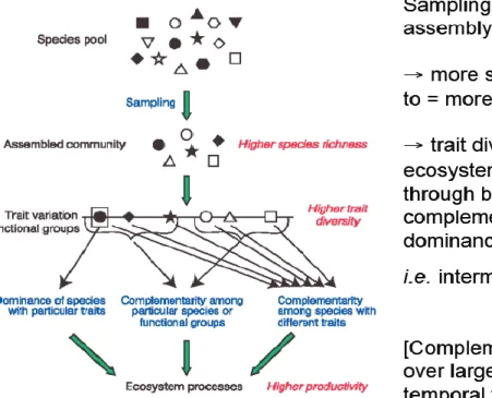
2.6 Greater diversity of species within a species pool is likely to result in a greater diversity of traits (for example different modes of feeding, reproduction, growth, survival etc.) and hence functional groups, which affects ecosystem processes through niche complementarity and dominance of particular subsets of complementary species (Loreau et al. 2001, and Figure 1)

4

The Ecosystem Approach is a strategy for the integrated management of land, water and living resources that promotes conservation and sustainable use in an equitable way. It was endorsed at the fifth Conference of the Parties to the Convention on Biological Diversity (CoP 5 in Nairobi, Kenya; May 2000/Decision V/6) as the primary framework for action under the Convention (IUCN, 2008).

(16)

16

Figure 1 Hypothesized mechanisms linking biodiversity and ecosystem functioning (Source: Loreau et al. 2001)

2.7 Manipulative studies to address the impacts of reducing biodiversity suggest that a large pool of species is requiredto sustain the assembly and functioning of ecosystems subject to increasing human pressures (see review by Loreau et al. 2001). Whether dependence of ecosystem functioning on diversity comes from the need for recruitment of a few key species from the regional species pool (most productive marine ecosystems are typically characterized by low species diversity) or is due to the need for a rich assortment of complementaryspecies within particular ecosystems (a detailed review of this is disputed, and beyond the scope of this study but see (Palumbi et al. 2009). Nonetheless there is broad agreement that diversity is important for reducing temporal variability in ecosystem functioning under changing environmental conditions (Kikkawa 1986, Schultze & Mooney 1993, Bengtsson 1998, Hooper et al. 2002, Bevilacqua et al. 2006). Diversity may also make a system less susceptible to invasive species because species-rich communities use available space, the limiting resource, more efficiently (Stachowicz et al. 1999).

2.2 Representative indicators of biodiversity

2.8 The Convention on Biological Diversity refers directly to „variability among living organisms‟ and stresses that this includes diversity within species as well as between species. The relationship between variety within a species and the number of species in a genus was first identified by Darwin, and the rate at which species are formed and the relative abundance of species in ecological communities was made explicit within the neutral theory of biogeography (as cited by Magurran 2005). Research has continued over the

(17)

17

decades to explore the relationship between genetic and species diversity and unravel the processes that underpin it (Vellend 2005).

2.9 At the other end of the scale, the relationships between habitat and landscape diversity (or heterogeneity) and species diversity have continued to be examined since Aldo Leopold first put forward his law of dispersion (principle of edge) in 1933 (Leopold 1933). Most studies have found a positive correlation between habitat heterogeneity and species diversity, although there is some dispute that empirical support is biased towards studies of vertebrates and habitats under anthropogenic influence (Tews et al. 2004). It could therefore be argued that whilst the most commonly accepted level for representing diversity are species, a measure of habitat diversity may be more representative of the whole community diversity of an area.

2.10 Species are by far the most common unit to represent biodiversity. In practice a convenient subset of the biota is usually assessed on the assumption that patterns in diversity of this subset correlate with overall biodiversity of the total species pool. This is conceptualized as surrogacy by Warwick & Clarke (2001) but we use the term surrogate measures later in this review to describe non-ecological physical surrogates. Apart from the obvious impracticalities of routinely sampling all species from microbes to mega fauna, it is also a reflection of management and conservation targets (i.e. few microbial or meiofaunal species appear on protected species lists).

2.11 A number of different multi-species surrogate measures for the total species pool have been proposed (Table 1). The correlation between these measures and total biodiversity however has only been tested in a few cases (Leonard et al. 2006).

2.12 Some studies have focussed on areas where the number of rare or declining species or habitats or other priority features is high; partly for cost effectiveness but also because it was assumed that by focusing on priority species there will be an effective umbrella for overall species richness area, which is not always the case (Bonn et al. 2002). Protecting structural or ecosystem engineer species may, however, be effective (Jones et al. 1997). 2.13 Additionally, biodiversity has been assessed using the biodiversity of certain

groups (e.g. molluscs) as a proxy for the entire marine community diversity. This approach has the advantage that the group is stable taxonomically and fairly evenly recorded but they are not necessarily indicators of total diversity (Smith 2008). An extension of this approach is to use „death assemblages‟ of shell-bearing molluscs, a technique often used to examine fossil records. In some cases a good relationship between the death assemblage and the diversity of the taxa in the area they originated from has been identified (Warwick & Light 2002), while others show inflated diversity compared with the living assemblage (Pandolfi & Greenstein 1997).

(18)

18

Table 1. Multi-species measures that have been proposed as surrogates for the biodiversity of the total species pool

Indicator Comments References

Selected taxa or taxon groups

Uses one or a subset of taxonomic groups (e.g. polychaetes, Malacostraca, sea birds, mammals, or sharks, that have well known taxonomy and are tractable to sample) to represent total biodiversity. This technique is well established in the terrestrial literature (e.g. Prendergast et al. 1993).

(Williams & Gaston 1994, Phillips 2001, Olsgard et al. 2003, Terlizzi et al. 2009)

Death

assemblages

Use of the remains of shell-bearing molluscs (gastropods and bivalves) in sedimentary habitats to indicate diversity patterns in original living communities.

(Warwick & Light 2002, Smith 2008)

Gut contents of key predators

Uses the concept of predators as biodiversity collectors and assumes that their gut contents reflect the biodiversity of prey items available (unvalidated).

(Féral et al. 2003)

Large

conspicuous species

Uses species that are conspicuous for visual census such as Pinna nobilis in Posidonia

meadows, assuming a relationship between conspicuous and cryptic diversity.

(Féral et al. 2003)

Functional (e.g. trophic) diversity

Uses the diversity of functional groups to infer patterns in overall biodiversity. Functional diversity reflects the biological complexity of an ecosystem and it can be argued that functional diversity may in fact be the most meaningful way

of assessing biodiversity while avoiding

cataloguing all species in marine ecosystems. By focusing on processes, it may be easier to determine how an ecosystem can most effectively be protected and in the process of protecting biological functions, many of the species that perform them will also be protected.

(Steele 1991, Leonard et al. 2006)

Diversity of rare or endangered

species

Uses the number of rare or threatened (priority) species or habitats as a surrogate for overall biodiversity. While this is not a true reflection of biodiversity, it can be a useful tool for managers to identify hotspots of priority features.

(Prendergast et al. 1993, Myers et al. 2000, Hiscock & Breckels 2007)

Endemic species Due to fewer and weaker barriers to dispersal

there are no marine species believed endemic to anywhere in the UK. It is therefore not an appropriate measure for assessing biodiversity hotspots in this instance

(Reid 1998, Myers et al. 2000, Phillips 2001, Hughes et al. 2002)

2.14 Genetic diversity is the variation in the amount of genetic information within and among individuals of a population, a species, an assemblage, or a community. It is reflected by the level of similarity or differences in the genetic makeup of individuals, populations and species. These similarities and differences may evolve as a result of many different processes e.g. chromosomal and/or sequence mutation, and physical or behavioural isolation of populations. Although genetic diversity is not always obvious, it is

(19)

19

extremely important as it is a requisite for evolutionary adaptation to a changing environment. Genetic diversity can be thought of as an insurance, which allows adaptation to changing environmental conditions. Recently there have been concerns for the loss of genetic diversity in commercially important fish species could have an impact on fisheries (Smith 1994).

2.15 Microbial diversity on earth is estimated to be between 103 – 109 species (Pedrós-Alió 2006). In marine systems, the diversity of microbes is the key to their unique metabolisms that allow microbes to carry out many steps of the biogeochemical cycles that other organisms are unable to complete. The smooth functioning of these cycles is necessary for life to continue, not just in the oceans but on earth. While the diversity in taxonomy and function of marine microbes is recognised, little progress has been made to describe them formally (Pedrós-Alió 2006).

2.3 Metrics for measuring marine diversity

2.16 There is considerable controversy surrounding the most appropriate measure to identify areas of high diversity, both in terrestrial and marine systems (Possingham & Wilson 2005). Each metric has different data requirements and benefits and disadvantages for its use (Table 2) and we review the main ones here (see Magurran 2004, Gray & Elliott 2009 for more comprehensive reviews of measures of species diversity). Compounding this problem of selecting the most appropriate metric is the lack of similarity between different metrics (Orme et al. 2005).

2.17 Globaltaxonomic richness can be viewed at three different scales.

 Point diversity, which is the diversity of a single sample (Whittaker 1972).

 Within-community (α) diversity, which is the diversity of a particular area, usually expressed as the number of species in that ecosystem (Whittaker 1972, Hooper et al. 2002, Price 2002, Worm et al. 2003).  β diversity is the comparison of diversity between ecosystems, often

measured as the amount of species change (Whittaker 1972, Vanderklift et al. 1998, Hooper et al. 2002) and also known as turnover diversity (Magurran 2004).

 γ diversity is a measure of overall diversity within a large region (Whittaker 1972, Vanderklift et al. 1998, Hooper et al. 2002).

2.18 In addition, diversity can be measured at different levels of biological organization, from genes to landscape, although in practice, species and habitats are the most common units.

(20)

20

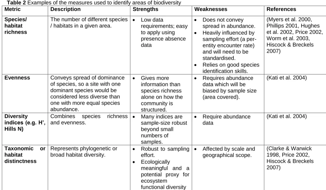
Table 2 Examples of the measures used to identify areas of biodiversity

Metric Description Strengths Weaknesses References

Species/ habitat richness

The number of different species / habitats in a given area.

 Low data

requirements; easy to apply using presence absence data

 Does not convey spread in abundance.  Heavily influenced by

sampling effort (a per-entity encounter rate) and will need to be standardised.

 Relies on good species identification skills.

(Myers et al. 2000, Phillips 2001, Hughes et al. 2002, Price 2002, Worm et al. 2003, Hiscock & Breckels 2007)

Evenness Conveys spread of dominance of species, so a site with one dominant species would be considered less diverse than one with more equal species abundance.

 Gives more information than species richness alone on how the community is structured.

 Requires abundance data which will be biased by sample size (area covered).

(Kati et al. 2004)

Diversity

indices (e.g. H’, Hills N)

Combines species richness and evenness.

 Many indices are sample-size robust beyond small numbers of samples.

 Require abundance data

(Kati et al. 2004)

Taxonomic or habitat

distinctness

Represents phylogenetic or broad habitat diversity.

 Robust to sampling effort.

 Ecologically

meaningful and a potential proxy for ecosystem

functional diversity

 Affected by scale and geographical scope.

(Clarke & Warwick 1998, Price 2002, Hiscock & Breckels 2007)

(21)

21

Metric Description Strengths Weaknesses References

Functional diversity

Currently no consensus on a measure to use for functional diversity. Taxonomic

distinctness may be a useful approximation.

 Useful as meets a number of policy objectives

 No consensus on the measure to use.

(Leonard et al. 2006, Akpalu 2009)

Higher taxonomic diversity

Identification of individuals in samples to target taxon (phylum, class, order) and indices calculated from

numbers of taxa and/or relative abundance.

 Quicker/cheaper to process samples to lower taxonomic resolution

 This technique has not been validated for biodiversity, only for environmental health.

(Heip et al. 1988, Williams & Gaston 1994, Gaston &

Blackburn 1995, Roy et al. 1996)

Rarefaction/ Accumulation curves

Allows a comparison of samples containing different numbers of individuals or samples. Curves are produced by repeatedly re-sampling the pool of „n‟ individuals or „n‟ of species that would be found in samples containing fewer and fewer individuals than the total sample. Steep curves

represent high diversity.

 A comparative measure that is sample size independent

 Assumes that the proportional composition of individuals from

different species is the same across sample sizes.

 Can only be used to compare taxon richness at comparable levels of sampling effort.

(Sanders 1968, Gotelli & Colwell 2001, Gray & Elliott 2009)

(22)

22

Turnover (beta) diversity

Represents between habitat diversity or extent of change in composition among the

samples of a set.

 Useful when

comparing regions that extend across different habitats  An alternative

measure when taking a

neighbourhood approach.

 Can be applied to presence absence data

 This technique is primarily used for comparing diversity along transects.  Beta diversity will be

high when differences in alpha diversity are large.

(Whittaker 1972, Koleff et al. 2003, Magurran 2004, Gray & Elliott 2009, Terlizzi et al. 2009)

Chao estimator Based on the concept that rare species carry the most

information about the number of missing ones.

 Robust to sampling effort.

 A potential measure to

examine sampling artefacts

 Sensitive to area and must limit spatial extent of samples used in its calculation.

 Assume homogeneity of samples so not suitable for comparing samples across different sites

(Chao & Shen 2003, Foggo et al. 2003)

(23)

23

2.3.1 Direct measures of species diversity

2.19 Species richness, the number of species at a given location, is arguably the most widely used and simplest measure of diversity and does not rely on abundance data being recorded.

2.20 Species richness alone does not account for the spread in abundance between different species. For example, a site with ten species but with one species dominating would be classed as less diverse than one where all species were found in equal abundance. This information is captured in species evenness indices such as Pielou's evenness index (Purvis & Hector 2000).

2.21 Other indices widely used to quantify diversity include the Shannon-Wiener Index. The advantage of this index is that it takes into account both the number of species and their evenness. The value of the index is increased either by having additional unique species, or by having greater species evenness. The disadvantage is that the measure requires abundance data. 2.22 Average taxonomic distinctness is a diversity measure that reflects how

different species are from each other at any given location (Warwick & Clarke 2001), representing the range of taxonomic groups that are present (phylogenetic diversity, see Box 1). For example, a sample consisting of ten species from the same genus would be seen as much less biodiverse than another sample of ten species, all of which are from different families. Unlike measures of species richness, the level of taxonomic relatedness is robust to variations in sampling effort and does not require abundance data.

(24)

24

2.23 Another approach is to use higher (taxonomic) level diversity to assess biodiversity in marine ecosystems (e.g. family-level richness Heip et al. 1988, Williams & Gaston 1994). The rationale behind this is: 1) diversity at high taxonomic levels is much greater in the sea where nearly all known phyla are represented (there are 14 phyla found only in marine ecosystems (Clarke & Warwick 2001)) and: 2) identification of species only to higher taxonomic levels is quicker and cheaper (Féral et al. 2003). Legandre and Legandre (1998) make a case that “in principle, diversity should not be computed on taxonomic levels other than species” because the resources of an ecosystem are apportioned among the local populations (demes) of the species present in the system, thus each species represents a separate genetic pool.

2.3.2 Metrics for measuring habitat diversity

2.24 The variety of different habitats in an area is another way of expressing biodiversity. This is based on the link between species richness and habitat diversity that is found at a variety of scales (e.g. Izsak & Price 2001, Hewett et al. 2002, Tews et al. 2004, Thrush et al. 2006). While conceptually there is a good argument for considering diversity at the level of habitats, pragmatically this can also help to fill in gaps in data coverage in species records and explain patterns found in species diversity where data overlap.

Box 1. Average taxonomic distinctness

Average taxonomic distinctness calculates the average taxonomic distance apart of all the pairs of species in a sample, based on branch lengths of a hierarchical Linnaean taxonomic tree (Warwick & Clarke 2001). The illustration below shows the principle of average taxonomic distinctness. Both samples have the same species richness with five species present. However, sample 2 has five species from the same genus, whilst sample 1 has five species from four different genera and three different phyla. Therefore species from sample 1 are separated by longer branch lengths in the taxonomic tree and have a greater average taxonomic distinctness.

(25)

25

2.25 Many measures developed for species can equally be applied to habitat diversity such as habitat richness (number of habitats at a location) and habitat distinctness. Locations with habitats from completely different habitat types can be considered more diverse than locations with similar habitats (i.e. from the same broad habitat group). Habitat distinctness was first applied in a UK wide assessment of marine benthic biodiversity by Hiscock & Breckels (2007). The measure works in the same way as average taxonomic distinctness (Clarke & Warwick 1998) to allow quantification of the variety of habitats present at any particular location, using the EUNIS hierarchical habitat classification (Box 2 and Box 3), which is similar in principle to the Linnaean tree for species taxonomy.

2.26 While a biotope is the smallest geographical unit of the biosphere or of a habitat that can be delimited by convenient boundaries and is characterized by its biota (Lincoln et al. 1998), it is arguably not the most suitable for quantifying habitat diversity from a practical viewpoint. This is because biotope classifications include information on the species assemblages present and the dominance of key species. Higher levels of the hierarchical classification (such as main habitat types, Box 2) may be more suitable in representing higher organisational levels of diversity without the bias of dominant species. 2.27 The different diversity metrics each have their own advantages, disadvantages

and data requirements (Table 2). Furthermore, there is an observed lack of congruence between measures (Orme et al., 2005). No one measure provides a complete representation of biodiversity. This has led to the combination of a range of measures being used to capture patterns in biodiversity (e.g. Reid 1998, Myers et al. 2000, Hiscock & Breckels 2007). 2.28 Some studies that have combined different measures have incorporated direct

measures of diversity with, for example, the number of endemic species5 and areas of threatened or declining habitats (Myers et al. 2000). The advantage of these combined approaches is that the resulting score or rank of biodiversity importance is simple for marine spatial planners to visualize. However, with the ongoing technological development of GIS, different biodiversity metrics (e.g. species richness, biotope distinctness, seabed type diversity etc.) can be held as separate layers within a decision support tool. A disadvantage of combined scores is in determining the weighting of different metrics. Decision-makers may well require to see the information that the score was based on, which can be effectively „lost‟ from the planning process when metrics are combined.

5

Endemism (where a species is restricted to a particular area) is an important criterion to identify hotspots on land and in fresh water but is an unusual feature in the marine environment of the north-east Atlantic due to fewer and weaker barriers to dispersal, and there are no marine species believed endemic to anywhere in the UK.

(26)

26

2.3.3 Spatial considerations

2.29 The number of species, or even habitats, present in any given area is a function of the size of that area (McGuinness 1984). This is a limitation of most of the metrics outlined above and is especially true for species richness; they are highly dependent on spatial scale (and sampling intensity – this is dealt with in section 2.3.4). In order to make comparisons of the levels of biodiversity, data must be standardised for spatial scale so that locations with high diversity can be identified.

Box 2. Description of the EUNIS classification system

The EUNIS classification was developed for the European Environment Agency in order to standardize the description of habitat types across Europe. It allows for harmonization of a number of classification schemes (including the Marine Biotope Classification for Britain and Ireland). The classification allows the identification of both artificial and natural habitats in the terrestrial, marine and freshwater environments. For the purpose of the EUNIS classification a habitat is described as “Plant and animal communities as the characterising elements of the biotic environment, together with abiotic factors operating together at a particular scale” [http://eunis.eea.europa.eu/about.jsp].

As a hierarchical classification it can be used at various levels of detail (see below). The JNCC have produced translation tables that match habitat types in the EUNIS habitat classification to the following schemes:

the marine habitat classification for Britain and Ireland (v04.05); EC Habitats Directive Annex I types;

OSPAR priority habitat types; and

UK Biodiversity Action Plan priority habitat types (Source: Joint Nature Conservation Committee, 2007)

Description of EUNIS classification levels

Level Description

1 Environment (marine):a single category is defined within EUNIS to distinguish the marine environment from terrestrial and freshwater habitats. 2 Broad physical habitats: based on depth and broad substrata (e.g. rock or

sediment) or water column e.g. littoral sediment. 3

Main habitats: mainly physical based on energy regime but with some general description of biogenic habitat e.g. Littoral sediments dominated by aquatic Angiosperms, and Sublittoral macrophyte dominated sediment 4 Dominant community type: community type described without specific

reference to conspicuous species e.g. Fuciods in tide swept conditions 5 Community: distinguished by their different dominant species or suites of

(27)

27

2.30 Several approaches have been taken to standardize the spatial scale in the area being assessed and these fall broadly into two types: 1) in some studies the area was broken down into even-sized grid units (grid size is generally dependent on resolution and coverage of survey data but management implications may also play a role in their spatial determination) to enable comparison across the area of interest (Worm et al. 2003, Orme et al. 2005, Langmead et al. 2008); and 2) other studies have used natural features as their sample units (e.g. Hiscock and Breckels 2007). In the latter approach, physiographic features were applied as the sample unit (islands, embayments, estuaries, linear coastlines and sea lochs). The main problem with this method is that some of these features may be substantially larger than others, meaning that diversity may be compared at a local level in some (α diversity) but regionally in others (β diversity), invalidating overall comparisons between areas.

2.31 Although there are no examples known to the authors, it is clearly possible to use different spatial resolutions for different areas or system components, driven again by data availability (sampling intensity). There are large differences in spatial and temporal resolution of data between the intertidal and subtidal, inshore and offshore, and the benthic system compared with the pelagic. Inherently there is a trade-off between using a small spatial unit (surveys so sparsely spread that many spatial units are empty) and using larger spatial units (losing resolution in the data), and determining the optimal grid cell size is for each type of data is an important step in biodiversity assessment (Stockwell & Peterson 2003), yet the reasoning for the choice of grid cell size is rarely given. General guidance from macro ecology promotes the use of re-sampling procedures to identify the optimal resolution (Rahbek Box 3. Example from the EUNIS hierarchical habitat classification system.

(28)

28

2005). It is clear that one size does not fit all with respect to the optimal spatial resolution for conducting biodiversity assessments, and consideration at different scales is particularly important when taking an integrated, multi-level systems approach to identifying areas of high diversity if important detail is not to be lost in „scaling up‟.

2.32 Finally, different shaped spatial grids have been used for mapping diversity, with either rectilinear (Roberts et al. 2002) or hexagonal units. The latter are commonly used for spatial planning (Bassett & Edwards 2003, Worm et al. 2003, Oetting et al. 2006). The argument in favour of hexagonal units suggests that they offer the best alignment to complex features thus providing a better level of coverage. In addition techniques have been developed to counter the bias of placing grids over complex landscapes and spatially auto correlated data sets. Overlapping or roaming grid squares and neighbourhood statistics „soften‟ the artificial edges and smooth errors which are an artefact of the grid placement, by taking adjacent cells into consideration in analyses (Dennis et al. 2002). Neighbourhood statistics involve combining data from surrounding cells into the central focal cell, thus the final value of each cell is influence not only by the data underlying that cell but also by its neighbours. This is important when you consider that species richness is not only influenced by the number of individuals but also by the species richness of the surrounding community.

2.3.4 Data quality and standardisation

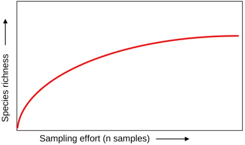
2.33 Estimates of areas of diversity are extremely dependent on the state of current knowledge: data coverage (discussed above), sampling effort and also the age of data sets (Magurran 1996, Worm et al. 2003). For species richness there are clear relationships with the number of samples, or put simply, the more effort spent searching for species, the more will be found (species accumulation curves, Figure 2). Species accumulation curves generally rise very quickly at first and then level off towards an asymptote as fewer new species are found per sampling unit collected.

2.34 Different statistical techniques have been employed to compensate for variable sample intensity in order to give a comparable unbiased estimate of relative biodiversity. These include rarefaction (Worm et al. 2003), regression analysis (Hiscock & Breckels 2007, Langmead et al. 2008) and re-sampling techniques such as Monte Carlo analysis (Moulins et al. 2008). There is a limit to the success of these techniques when faced with extremely low sample numbers, and some studies have omitted areas with extremely low numbers of surveys by setting a lower limit to the number of surveys per spatial unit (Langmead et al. 2008). In addition, the Chao 2 estimator measure is based on the concept that rare species carry most information about the number of missing ones, and has been applied to look for artefacts in data sets caused by this (Foggo et al. 2003).

(29)

29

Figure 2 species accumulation curve showing relationship between the species richness and sampling effort.

2.35 With benthic marine data sets, the number of species can be closely linked to the type of habitat, and the sampling technique employed. Samples collected using a benthic core sample and sieved using a 0.5 mm sieve are likely to have greater diversity than samples collected using a trawl, drop down camera or diver surveys. Thus sub-setting data for standardization facilitates like-with-like comparisons of diversity that are not simply an artefact of the data collection technique. In a study by Langmead et al. (2008), data were split by physiographic type to account for such differences (e.g. rocky areas were only compared with other rocky areas) and sites of high and low diversity were identified for each main physiographic type. These estimations were combined for all physiographic types to build up a picture of benthic biodiversity (irrespective of habitat) for the entire Firth of Clyde. Building on this approach, further work has been carried out to classify the methods employed to collect benthic data into broad groups and compare diversity measures only within these groups to remove the bias inherent in the sampling methodology (Jackson et al. in progress).

2.4 Surrogate measures for marine pelagic biodiversity

2.36 All the measures in the previous section are more or less direct measures of the biodiversity of an area, and have mostly been applied to benthic systems. Measures previously proposed to indicate pelagic diversity reflect the fact that most marine pelagic ecosystems have a relatively simple structure, with energy flowing from phytoplankton primary producers, through zooplankton (often dominated by copepods) to pelagic schooling fishes, and finally to a variety of top predators including fishes, marine mammals and seabirds (Jennings et al. 2001). These were:

Sampling effort (n samples)

S

p

e

cies

ri

ch

n

e

(30)

30

i. Diversity measures for different system components including phytoplankton, zooplankton, fish, cetaceans and seabirds;

ii. Satellite earth observation (EO) surrogate measures (thermal fronts, sea surface temperature (SST) and ocean colour);

iii. Indicators such as pelagic mega fauna (e.g. basking sharks).

2.37 Earth Observation data (SST, thermal fronts and ocean colour) have high spatio-temporal coverage and fine spatial resolution, which is lacking for most other pelagic measures (apart from Continuous Plankton Recorder data on plankton). In addition, EO data has been correlated with overall pelagic diversity, whilst others are restricted to being measures of specific system components and as such are not reviewed here (but see Appendix 3).

2.4.1 Thermal fronts

2.38 The influence of oceanic fronts on biological productivity has long been studied. Pingree (1977) noted that the stratified side of tidal fronts could support dense phytoplankton blooms throughout the summer due to the rare combination of high nutrients and light. Further into the stable stratified region nutrient levels remain depleted after the spring bloom; and on the well-mixed side of the front the plant cells receive a much lower mean light level which outweighs the relatively high nutrient levels. Bakun (1996) identified fronts as important structures that could result in the „triad‟ of enrichment, concentration and retention of nutrients.

2.39 Relationships have been established between fronts and fish abundance, for instance swordfish (Podesta et al. 1993), tuna and billfish (Worm et al. 2005). In addition, Worm et al. (2005) determined a global correlation of predator diversity with fronts. Although no studies have found a correlation between fronts and overall diversity, higher predator diversity has been linked to biodiversity in the open ocean (Worm et al. 2005).

2.40 Fronts that extend to the sea surface may be observed by satellite if the water masses differ in temperature or colour. This remote sensing of fronts has enabled a process-based understanding of mesoscale population dynamics capable of explaining regime shifts (Bakun 2006, ICES 2006). Remote sensing of fronts is promoted as a key tool in determining marine habitat hotspots (Palacios et al. 2006, Sydeman et al. 2006). Since identifying fronts in satellite images manually is a tedious and subjective task, several researchers have proposed image processing algorithms to do this semi-automatically (e.g. Simpson 1990, Bardey et al. 1999), or entirely automatically (Cayula & Cornillon 1992). A few authors have superimposed the locations of all fronts detected on a sequence of images to produce a single combined map (e.g. Podesta et al. 1993, Ullman & Cornillon 1999). Miller (2004, in press) extended this methodology to visualise both dynamic and stable fronts, generating metrics to indicate their temperature gradient, persistence and proximity to other observations.

(31)

31

2.4.2 Sea Surface Temperature (SST)

2.41 Apart from the use of EO-derived SST for locating oceanic fronts, the range of SST values has also been applied as a surrogate for fish abundance. Most species have a preferred temperature habitat, so this can help define their spatial distribution e.g. for tuna (Zainuddin et al. 2008), or represent coastal retention events for pilchard, sardine and anchovy stocks (Cole 1999). The most generic relationship between SST and fish abundance is that caused by coastal upwelling, bringing nutrient-rich deep water to the surface. Upwelling zones can support much greater biodiversity. Upwelling zones are a regionally important feature with small zones around the south west of the UK (off Cornwall) influencing productivity. EO SST time-series data of upwelling events have been related to studies of zooplankton and fish larvae in Galicia (Tenore et al. 1995), Portuguese swordfish, tuna, sardine and mackerel (Santos et al. 2001, Santos et al. 2006), but few studies have correlated SST or upwellings with levels of diversity.

2.4.3 Ocean colour

2.42 Chlorophyll-a is a good estimator of phytoplankton abundance. Various EO models can be used to estimate primary production. EO models using chlorophyll-a, light (photosynthetically active radiation (PAR)) and SST can quite accurately estimate surface primary production, and these are well summarised by (McClain 2009). Higher productivity may support high pelagic diversity; this may also impact on benthic productivity and biodiversity.

2.43 However, there are issues with this technique since standard algorithms for chlorophyll-a retrieval from EO ocean colour, while accurate for the open ocean, suffer errors in turbid shelf seas where suspended sediment and coloured dissolved organic matter mask the chlorophyll signal. This can result in exaggerated chlorophyll-a values near estuaries, reducing the value of standard chlorophyll-a maps for monitoring phytoplankton in shelf seas. Several algorithms have been proposed to tackle this problem: the empirical OC5 algorithm (Gohin et al. 2002) corrects the chlorophyll-a signal by estimating and removing the radiance contribution from suspended sediment, significantly reducing these errors in turbid water.

2.5 Predictive techniques

2.44 Biological survey data is relatively sparse, particularly in inaccessible and offshore areas, and different approaches to the „data-hungry‟ measures outlined above have been researched. One possibility is the use of predictive maps of broad scale habitats and environmental parameters to identify potential areas of high diversity where survey data do not exist.

(32)

32

2.45 For the terrestrial environment there are well established theoretical reasons why environmental variables should be good estimators of the spatial distribution patterns of species richness, supported by empirical studies (Austin 1985, Austin et al. 1990, Prendergast & Eversham 1997, Margules & Pressey 2000). Models and statistical techniques developed in terrestrial ecology to compare how well different environmental surrogates reflect diversity (Margules & Austin 1994, Gioia & Pigott 2000, Elith et al. 2006) are applicable to the marine environment, where theories on why high diversity areas occur where they do are beginning to emerge from analyses of data on global and continental scales. Orme et al. (2005) argue that the ecological, evolutionary and human effects that underlie the origin and maintenance of biodiversity are largely associated with large-scale topography.

2.46 A number of projects to map marine species distributions by modelling relationships with marine habitat and environmental information (e.g. Sandman et al. 2008, Vaz et al. 2008 and HabMap, http://habmap.org). The obvious extension to modelling individual species distributions is to combine them to create maps of richness (Stockwell & Peterson 2003). Predictive species maps are however only possible for species with a clear relationship to certain environmental characteristics and aggregations of species maps do not account for density dependent factors and other species interactions. 2.47 Developments in satellite remote sensing and a geographic information

system (GIS) coupled with spatial statistical software allow the efficient characterization of biodiversity at landscape level using geospatial techniques. Roy & Tomar (2000) predicted biological richness at landscape level as a function of habitat, biogeographical setting, disturbance regime and environmental complexity. Top-down rule-based approaches, which combine environmental variables, such as depth, productivity, seabed type and current speed, can be used to classify areas of the seabed into different broad habitat types. This technique has been used for broad scale national and international projects such as UKSeaMap (Connor et al. 2006) and MESH6. Such predictive seabed habitat maps could be used to look at landscape diversity. However, the quality of predictive seabed habitat maps (or model that underpins it) is related to the data used to construct it.

2.48 Problems with data availability and a lack of robust relationships between species and environmental conditions, particularly at larger spatial scales have led researchers to examine alternative approaches. For example modelling and predicting potential underlying drivers of high diversity, e.g. productivity and disturbance regimes (Loreau et al. 2001, Chase & Leibold 2002).

2.49 Comparisons of different predictive methods have shown divergent results (Stockwell & Peterson 2003) attributable to differences in analytical methods, geographical scales and biogeographical histories of the study areas.

6

(33)

33

Reliable generalizations and an understanding of how such factors affect taxonomic surrogacy are still developing for the marine environment.

2.50 In summary, predictive methods have the potential to identify important areas of diversity where survey data is limited or absent. However, any predictive method requires substantial validation and with an uncertainty still surrounding the reliability of predictive approaches conservation managers are unlikely to base decisions on the location of MPAs on predicted map layers without considerable validation and resurvey.

2.6 Hotspots of biodiversity

2.51 In 1988, the British terrestrial biologist Norman Myers initiated the use of the term "biodiversity hotspot" as a biogeographic region characterized both by exceptional levels of plant endemism and by serious levels of habitat loss (Myers 1988). Since then the term “biodiversity hotspot” has been used to describe the relatively high occurrence of a single species, diversity of species within a certain group (realm, trophic level, size class), of ecosystem services or of productivity.

2.52 In an assessment of biodiversity hotspots carried funded by WWF, Breckels and Hiscock (2007) used the definition:

“Marine biodiversity hotspots are areas of high species and habitat richness that include representative, rare and threatened features”.

2.53 The main drawback with the hotspots approach is that the threshold at which a location is identified as a “hotspot” is often subjective or ambiguous, and can be related to 1) conservation objectives and 2) the area of search, which limits the range of diversity for example the number of species within the species pool increases with area of search making a local hotspot cooler. In addition there can be confusion in the use of the term „hotspots‟ with other types of hotspot, such as hotspots of productivity (Valavanis et al. 2004) and single species abundances (Sims et al. 2003, Evans & Wang 2008), which may be unrelated to biodiversity sensu stricto.

2.7 Summary and conclusions

2.54 The preceding sections provide a critical review of approaches for identifying areas of high marine biodiversity in both the benthic and pelagic realms. The review identifies various measures to assess marine diversity (e.g. diversity indices, number of species, number of priority species and taxonomic distinctness) and highlights the importance and limits of data quality and coverage. The review also identifies the necessity, not only to employ effort standardisation techniques, but also to validate and present the level of confidence given to the layer.