Sharif University of Technology
Scientia IranicaTransactions B: Mechanical Engineering www.scientiairanica.com
An ecient concept for non-dimensionalizing the
dung equations based on the parameterized
perturbation method
A. Afsharfard
a;b;and A. Farshidianfar
ba. Department of Mechanical Engineering, University of Torbat-e-Heydarieh, Torbat-e-Heydarieh, Iran. b. Department of Mechanical Engineering, Ferdowsi University of Mashhad, Mashhad, Iran.
Received 5 October 2011; received in revised form 5 March 2013; accepted 25 May 2013
KEYWORDS Nonlinear ordinary dierential equation; Perturbation method; Characteristic distance;
Non-dimensionalization.
Abstract. In this paper, ongoing studies to investigate nonlinear Ordinary Dierential Equations (ODE) are extended by presenting a new concept in non-dimensionalization process. This concept is illustrated with a practical example of nonlinear ODEs, which cannot reliably solve using the numerical methods. In this paper, two perturbation techniques are used to solve the problem. Eect of varying the dimensionless initial displacement on the accuracy of solution is investigated. It is shown that if the process of non-dimensionalizing is done appropriately, the calculated results will be extremely accurate. Moreover, a new concept called \behavior of results" is proposed to nd accurate results.
© 2013 Sharif University of Technology. All rights reserved.
1. Introduction
Mathematical modeling can be used to simulate the behavior of the practical systems and provide a better understanding of them [1]. Theoretical investigations are useful for drawing general conclusions from simple models [2]. In reality, every physical process is a nonlinear system and should be described by nonlinear equations. Kerschen et al. studied the sources of nonlinearity, and classied them [3].
Nowadays, there is a large tendency toward nu-merical simulation of nonlinear systems [4-6]. The reason for this interest lies in the growth of powerful computers. However, it should be considered that the numerical methods require a considerable number of iterations in order to approach the true solution, and it is necessary to provide initial estimates of the unknowns [7]. Due to the limitations of numerical
*. Corresponding author. Tel.: +98-511-8695553 E-mail addresses: [email protected] (A. Afsharfard), [email protected] (A. Farshidianfar)
methods, it is necessary to nd analytical solutions for nonlinear problems.
In spite of linear problems, it is very dicult to nd analytical solution for nonlinear equations. Consequently, many eorts have been made to develop the methods of studying nonlinear systems. Nayfeh and Mook [8], Verhulst [9] and Rand [10] studied nonlinear equations.
Perturbation methods provide powerful tools to analyze nonlinear problems [11-14]. Ganji et al. applied the perturbation methods to solve nonlinear equations in uid mechanics problems [15-17]. They also evaluated a nonlinear engineering system, using the so-called amplitude-frequency formulation, which overcomes the diculty of computing the periodic behavior of such systems [18]. But, as well as other nonlinear techniques, the perturbation methods have several limitations. Nayfeh [19] and O'Malley [20] investigated the restrictions of perturbation methods. Usually, before using the perturbation methods, this question may be arisen: \which technique, out of presented perturbation methods, is better than the
others?" Finding an answer for this question is not easy, because some special nonlinear problems may be accurately solved using a particular perturbation technique [21,22]. The main motivation of the present work is to nd a reasonable answer for the above question.
Consider a plasma tube in which the magnetic eld is cylindrical and increases toward the axis in inverse proportion to the radius. A nonlinear equation describes the motion of injected electrons into the dis-cussed plasma tube. In this paper, the nonlinear equa-tion is solved using two perturbaequa-tion techniques [23]. Parameterized perturbation and iteration perturbation methods are used to solve the nonlinear ODE. It is shown that wavelength of the motion can be exactly approximated using the iteration perturbation method. Finally, eects of the process of non-dimensionalizing on the accuracy of solution, which is obtained using the parameterized perturbation method, are investigated and discussed.
2. Mathematical modeling
The orbit of a charged particle q moving in an electric and magnetic eld can be formulated using the Lorentz force equation [24]. This equation can be shown as follows:
F = q(E + v B); (1) where F is the Lorentz force, E is the electric eld, B is the magnetic eld and v is the instantaneous velocity of the particle. Consider the uniform magnetic eld (E = 0) in a plasma tube in which the magnetic eld changes cylindrically and increases toward the axis in inverse proportion to the radius. Therefore, the Lorentz force equation can be simplied to the following form:
F = qvC=r; (2)
where C is a constant, which relates to the magnetic eld (B). Variable r is the distance to the center line of the plasma tube. According to the Newton's second law, motion of the charged particle injected into the plasma tube can be given by:
mr;tt+ Cqvr 1= 0; (3)
where m is the mass of the charged particle. For convenience, the above equation can be rewritten as the following relation:
r;tt+ r 1= 0: (4)
In the above equation = Cqv=m. Consider u = r=r0
and = !0t, where r0 is the characteristic distance
and !0 is the natural circular frequency of vibration.
Therefore, dimensionless form of the above equation can be written as follows:
u;tt= u 1; (5)
where is equal to =!2
0r20. In the present study, the
initial conditions are assumed to be u(0) = A and u;(0) = 0.
3. Analytical solution
3.1. Iteration perturbation method
Iteration perturbation method is a relatively new perturbation technique coupling with the Iteration method [25]. The iteration formula for the dimension-less governing equation can be dened as follows:
(u)n+1+ "(u)n+1(u)2n = 0; (6)
where " is an introduced articial parameter and subscript n represents the nth order of solution. Com-paring between Eqs. (5) and (6), it can be concluded that, in this section, the articial parameter (") is equal to one. Assume that the initial approximate solution is u0 = A cos !t, where ! is the angular frequency of
the oscillation. Therefore, Eq. (6) can be rewritten as follows:
u;+ 2A 2u + "u;cos(2!) = 0; (7)
where " is an introduced articial parameter. The above equation is a sort of the Mathieu equation. Suppose that:
u = u0+ "u1+ "2u2+ ; (8)
2A 2= C
0+ "C1+ "2C2+ (9)
In the above equation it should be noted that the pa-rameter C0is equal to square of the angular frequency
(C0 = !2). Substituting Eqs. (8) and (9) into Eq. (7)
and equating the coecients of the same power of " results in the following dierential equation for u1:
u1;+ !2u1+
C1A A! 2
2
cos !
A!2
2 cos 3! = 0: (10) Vanishing secular term requires C1= !2=2.
Substitut-ing C1 into Eq. (9) results in:
! =A2 r
3: (11)
Therefore, the rst approximate wavelength of the charged particle motion is equal to:
= 5:4414pA
Neglecting the secular term and solving Eq. (10) with initial conditions u1(0) = 0 and u1;(0) = 0 yields the
following result:
u1= 16A (cos ! cos 3!) : (13)
Substituting Eq. (13) into Eq. (8) results in the follow-ing relation:
u1= A cos ! +16A(cos ! cos 3!): (14)
If the above solution is substituted into Eq. (6) as the 0th order solution, the following relation will be obtained:
u; + 256"uA 2(17 cos ! cos 3!) 2= 0: (15)
The above equation can be rewritten as follows:
u; +256145A 2u + " 5158cos 2! 14517 cos 4!
+2901 cos 6! !
u; = 0: (16)
Therefore, the circular frequency of motion can be expanded, as shown in Eq. (17).
256
145A 2= C0+ "C1+ "2C2+ (17) where C0 = !2. Substituting Eqs. (8) and (17) into
Eq. (16) results in the following dierential equation:
u1;+ !2u1+ C1u0+ 5158cos 2! 14517 cos 4!
+2901 cos 6! !
u0; = 0: (18)
The 0th order solution, in the above relation, can be replaced by what is shown in Eq. (14). Therefore, Eq. (18) changes to the following equation:
u1;+ !2u1+ 1716AC1 11734640A!2
! cos !
+ 1 16AC1
937 2320A!2
! cos 3!
+17A!92802 1160357 cos 5!
323
9280cos 7! + 9
9280cos 9! !
=0: (19)
Neglecting the secular term requires C1 = 69!2=290.
Regarding the parameter C1, presented in Eq. (17),
second order angular frequency can be calculated as follows:
! = A1 r
512
359 : (20)
Therefore, the wavelength of motion is equal to:
= 5:2612pA
: (21)
For convenience, very small coecients in Eq. (19) can be neglected. Therefore, this equation can be rewritten as follows:
u1;+ !2u1' 16067A!2cos 3!
6069
10764800A!2cos 5!: (22) The second iterative solution of Eq. (5), which is calculated using the iteration perturbation method, is given in Eq. (23). For convenience, the second iterative solution of problem is briey named as \second order" solution.
u() =17A16 cos ! 147A1280 cos 3! 6069A
258355200cos 5!: (23) 3.2. Parameterized perturbation
Initially, Eq. (5) is multiplied by u2, then term 0:u ;,
which is equal to zero is added to the left side of this equation. Finally, all right side term of the equation is moved to the left side. Therefore, the new presentation for the dimensionless form of Eq. (5) can be shown as follows:
0:u;+ u2u;+ u = 0: (24)
Consider linear transformation u = "v, where " is an introduced perturbation parameter. Therefore, the above equation can be rewritten as follows:
0:"v;+ "3v2v;+ "v = 0: (25)
Expanded form of the parameters v, and 0 are given by:
v = v0+ "2v1+ "4v2+ (26)
= !2+ "2!
1+ "4!2+ (27)
0 = 1 + "2b
Substituting Eqs. (26), (27) and (28) into Eq. (25) and equating the coecients of same powers of ", yields the following relations:
v0;+ !2v0= 0; v0(0) = A" 1;
v0;(0) = 0; (29)
v1;+ !2v1+ v20v0;+ !1v0+ b1v0; = 0
v1(0) = 0; v1;(0) = 0; (30)
v2;+ !2v2+ (b2+ 2v0v1)v0;+ (b1+ v20)v1;
+ !1v1+ !2v0= 0;
v2(0) = v2;(0) = 0: (31)
If v0 that is calculated by Eq. (29) is substituted into
Eq. (30), the following relation will be obtained: !1=
b1+34A2" 2
!2: (32)
The parameter can be achieved by substituting the above equation into Eq. (27).
= !2+ "2b
1+34A2" 2
!2: (33)
In the rst order of solution, b1 = " 2. Substituting
b1 into the above relation and simplifying it results in:
! = p A r 4
3: (34)
Therefore, the wavelength of motion is as follows: = 5:4414pA
: (35)
To solve Eq. (31), the variable v1can be calculated by
Eq. (30). The variable v1 is equal to:
v1= A3" 3(cos ! cos 3!): (36)
Substituting Eqs. (32) and (36) into Eq. (31) results in:
v2;+ !2v2+ A! 2b
2
"
A3!2b 1
32"3 +
A5!2b 2
64"5
+A32"3!31 +A!"2 !
cos !
+ 19A128"5!52 +9A32"3!32b1 A32"3!31 !
cos 3!
+ 11A128"5!52 !
cos 5! = 0: (37)
Neglecting the secular term, in the above relation, needs to vanish the coecient of cos !. Therefore, the following equation will be constructed:
A!2 A!2b2
" + A3(!
1 !2b1)
32"3 +
A5!2b 2
64"5 = 0: (38)
Substituting b1 and ! (which are obtained previously
in Eq. (34)) into the above equation and simplifying it results in:
!2= !2
b2 1285 A 4
"4
: (39)
Regarding Eq. (27), the following equation can be concluded:
= (1 + "2b
1+ "4b2)!2+34A2!2 1285 A4!2: (40)
The above relation can be simplied to the following form (Regarding to Eq. (28)):
= !23
4A2 5 128A4
: (41)
The angular frequency of motion can be written as follows: ! = p A 2 p
3q1 5 96A2
: (42)
Therefore, the second order wavelength of motion is equal to:
= 5:4414pA
r
1 965 A2: (43)
Second order solution of Eq. (5), which is calculated using the parameterized perturbation method, is as follow:
u() =
A 128A3 +11A7685 cos ! A3 128 11A5 1024 cos 3! 11A5 3072 cos 5!: (44)
4. Results and discussions
A practical nonlinear ODE has been derived and solved using two perturbation techniques. The presented perturbation methods can be employed to solve various kinds of nonlinear problems. Here, this question may be posed: \why is the discussed kind of nonlinear dierential equations selected to be solved in this paper?".
The reason for this selection lies in the following facts:
As shown in Section 2, practical problems can be described using the discussed nonlinear dierential equation.
Numerical methods may wrongly solve the discussed nonlinear ODE. Therefore, it is necessary to nd analytical solution.
Exact wavelength of motion for the discussed prob-lem can be calculated. This will be used to verify the calculated results.
As said, among the above notes, numerical methods may be unable to solve the presented problem. The reason for this inability may lie in the fact that the concavity (u;) approaches to innity when the
vibratory particle passes from the origin (u = 0). Figure 1 shows the result of using several numerical methods for solving the discussed problem.
For the discussed problem, the wavelength of motion can be calculated, analytically. For this reason, consider u; = u;(u;);uand substitute it into Eq. (5).
Therefore, the exact wavelength of motion is equal to [22]:
exact=
r 2
Z A
0
du p
LnA Lnu = 5:0133 A p
: (45) Wavelengths of motion, which are achieved by em-ploying the iteration perturbation, are illustrated in Figure 2. It should be noted that the linear wavelength of motion (0th order) is obtained by neglecting the nonlinear term of Eq. (24). In doing so, to nd the linear wavelength of motion, term u2u
; is removed
from Eq. (24). With regard to Eq. (28), the equivalent linear form of Eq. (24) can be re-written as follows:
u; +1 + "2b
1+ "4b2+ u = 0: (46)
Note that in the linear problem, the introduced pertur-bation parameter (") can be considered negligible, so the equivalent linear wavelength of motion is equal to 2A 1=2. A curve that is obtained, using the cubic
Figure 1. Result of solving the governing equation, using several numerical method and perturbation method.
Figure 2. Behavior of the non-dimensional wavelengths with the order of solution.
spline interpolation, is tted to the calculated results. The spline curve will be used to describe the so-called \behavior of the calculated results", and it is obtained using the curve tting toolbox in MATLAB software.
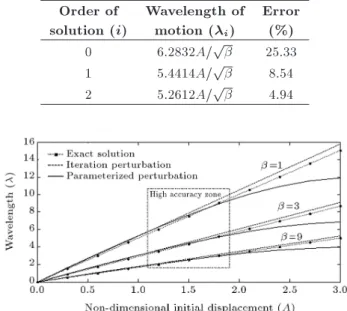
The calculated wavelengths of motion are com-pared with the exact solution in Table 1. As shown in this table, increasing the order of solution leads to nding more accurate results.
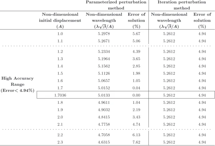
Wavelengths of motion, which are calculated using the parameterized perturbation method, are presented in Table 2. As shown in this table, in contrast with the iteration perturbation, the error of the second order solution of the parameterized perturbation method is variable with the parameter A. The second order wavelength calculated, using the parameterized perturbation method, is illustrated in Figure 3. It can be shown that if the dimensionless initial displacement (A) is selected between 1.120 and 2.114, the parameterized perturbation results will be
Table 1. Calculated wavelengths of motion, using the iteration perturbation method.
Order of solution (i)
Wavelength of motion (i)
Error (%)
0 6:2832A=p 25.33
1 5:4414A=p 8.54
2 5:2612A=p 4.94
Figure 3. Variation of the wavelength versus initial displacement.
more accurate than the result of the iteration pertur-bation method. This range, which is simply named \high accuracy zone", can be calculated regarding the exact solution.
Variation of error of the second order solution with varying the non-dimensional initial displacement (A) is shown in Table 3. As shown in this table, unlike the iteration perturbation method, error of solution in the parameterized perturbation method varies with changing the non-dimensional initial displacement (A). As said before, in the high accuracy range, the error of second order solution of the parameterized perturba-tion method becomes lower than the error of second order solution of the iteration perturbation method (4.94%). Furthermore, in this table it is shown that if A = 1:7036, the calculated wavelength of motion, which is achieved using the parameterized perturbation method, is equal to the exact solution.
Here, this question may be arisen: \can the
so-called high accuracy range be obtained without nding the exact solution?".
Finding an answer for the above question is really important, because the exact solution cannot be found for all nonlinear problems. To nd the relatively exact solution, it should be noted that the dierence between the higher order wavelengths of motion (which are obtained using the perturbation method) should be smaller than the lower order solutions. In other words, the following conditions should be fullled:
(I) j0 1j > j1 2j
(II) j2 3j < j1 2j
Therefore, the dierence between the second order solution and the rst order solution should be smaller than 0:8418A 1=2 (Condition (I)). This range, which
is simply named \acceptable range for non-dimensional initial displacement" is shown in Figure 4.
Table 2. Calculated wavelengths of motion, using the parameterized perturbation method. Order of solution (i) Wavelength of motion (i) Error (%)
0 6:2832A=p 25.33
1 5:4414A=p 8.54
2 5:4414p1 5A2=96A=p 108:54p1 5A2=96 100
Table 3. Error of using the second order solution with varying non-dimensional initial displacement. Parameterized perturbation
method
Iteration perturbation method
Non-dimensional initial displacement
(A)
Non-dimensional wavelength
(p=A)
Error of solution
(%)
Non-dimensional wavelength
(p=A)
Error of solution
(%)
High Accuracy Range (Error< 4:94%)
1.0 5.2978 5.67 5.2612 4.94
1.1 5.2671 5.06 5.2612 4.94
. . . .
1.2 5.2334 4.39 5.2612 4.94
1.3 5.1964 3.65 5.2612 4.94
1.4 5.1562 2.85 5.2612 4.94
1.5 5.1126 1.98 5.2612 4.94
1.6 5.0657 1.05 5.2612 4.94
1.7 5.0152 0.04 5.2612 4.94
1.7036 5.0133 0.00 5.2612 4.94
1.8 4.9611 1.04 5.2612 4.94
1.9 4.9032 2.19 5.2612 4.94
2.0 4.8415 3.43 5.2612 4.94
2.1 4.7758 4.74 5.2612 4.94
. . . .
2.2 4.7058 6.13 5.2612 4.94
Table 4. Dierence between the calculated dimensionless wavelengths.
(A) j0 1jp=A j1 2jp=A j2 3jp=A Note (I) Note (II)
1.0 0.8418 0.1436 0.5508 Satised
-1.5 0.8418 0.3288 0.0398 Satised Satised
2.0 0.8418 0.5999 0.7807 Satised
-2.5 0.8418 0.9726 1.1148 -
-Figure 4. Variation of the dierence and the
non-dimensional wavelength versus initial displacement.
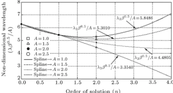
Figure 5. Behavior of the non-dimensional wavelengths with varying the parameter A.
Regarding the above two conditions, to nd the so-called high accuracy range for the non-dimensional initial displacement (A) can be calculated. Eect of varying the variable A on the behavior of the parameterized perturbation results is illustrated in Figure 5.
Dierence between the calculated dimensionless wavelengths of motion is presented in Table 4. As shown in this table, if A = 1:5, both of the two presented notes are satised. Therefore, error of the results that is obtained using the second order solution of the parameterized perturbation method, is equal to 1.98%. This solution is more accurate than the results which are obtained using the second order solution of the iteration perturbation method (4.94%).
Variation of the dimensionless distance (u) versus dimensionless time (), which is calculated using the second order solution of Eq. (5), is shown in Figure 6. In this gure, the initial dimensionless distance (A) is equal to 1.7, and the iteration perturbation and
Figure 6. Variation of the dimensionless distance with the dimensionless time (A = 1:7).
parameterized perturbation solutions are respectively plotted according to Eqs. (23) and (44).
5. Conclusion
This paper studies a practical nonlinear ordinary dif-ferential equation that describes the behavior of a particle, which is excited in a plasma tube. The discussed nonlinear equation cannot reliably be solved using numerical methods. For this reason, the govern-ing equation has been solved analytically, usgovern-ing two perturbation techniques.
Both of the rst and the second order solutions of the iteration perturbation method provide accurate results. Simplicity and accuracy of the iteration perturbation method makes it appropriate for practical applications. However, it has been shown that the so-called \behavior of results" in the iteration perturba-tion method, presented in this paper, is not acceptable. Unlike the iteration perturbation method, ac-curacy of the parameterized perturbation result is variable with the dimensionless initial displacement. It is shown that in a special range of the dimensionless initial displacements, the parameterized perturbation method provides extremely accurate results. This range is approximated using the concept of results behavior.
Nomenclature
A Initial dimensionless distance B Magnetic eld
C Constant E Electric eld
F Lorentz force P Coecient B Coecient
M Mass of the charged particle N Order of solution
Q Charged particle S Independent variable T Time
R Displacement of the charged particle U Dimensionless distance to the center
line of the plasma tube (r=r0)
V Instantaneous velocity of the particle X Independent variable
R Distance to the center line of the plasma tube
r0 Characteristic distance
Greek symbols Cqv=m =!2
0r02
" Coecient
wave length of motion T Dimensionless time ( = !0t)
Circular frequency
!0 Natural frequency of system
Subscripts
0 Initial conditions Exact Exact solution
References
1. Timmons, D.L., Johnson, C.W. and McCook, S.M., Fundamentals of Algebraic Modeling: An Introduction to Mathematical Modeling with Algebra and Statistics, 5th Ed. Brooks/Cole, Belmont, Calif. (2010).
2. Bender, E.A., An Introduction to Mathematical Mod-eling, Dover Publications, Mineola, N.Y. (2000).
3. Kerschen, G., Worden, K., Vakakis, A.F. and Golinval, J. \Past, present and future of nonlinear system iden-tication in structural dynamics", Mechanical Systems and Signal Processing, 20, pp. 505-592 (2006).
4. Afsharfard, A. and Farshidianfar, A. \An ecient method to solve the strongly coupled nonlinear dierential equations of impact dampers", Archive of Applied Mechanics, 82(7), pp. 977-984 (2012). doi:10.1007/s00419-011-0605-1
5. Kerschen, G. and Golinval, J.C. \A model updating strategy of non-linear vibrating structures", Interna-tional Journal for Numerical Methods in Engineering, 60(13), pp. 2147-2164 (2004). doi:10.1002/nme.1040
6. Steinbach, O., Numerical Approximation Methods for Elliptic Boundary Value Problems: Finite and Bound-ary Elements, Springer, New York (2008).
7. Ayyub, B.M. and McCuen, R.H., Numerical Methods for Engineers, Prentice Hall, Upper Saddle River, N.J. (1996).
8. Nayfeh, A.H. and Mook, D.T. \Nonlinear oscillations", Pure and Applied Mathematics, Wiley, New York (1979).
9. Verhulst, F., Nonlinear Dierential Equations and Dynamical Systems, 2nd Rev. and Expanded Ed. Universitext., Springer, Berlin, New York (1996).
10. Rand, R.H., Lecture Notes on Nonlinear Vibrations, Cornell University (2005).
11. Murdock, J.A., Perturbations Theory and Methods, John Wiley & Sons Inc., (1991).
12. Nayfeh, A.H., Perturbation Methods, Wiley classics library Ed., John Wiley & Sons, New York (2000).
13. Rand, R.H. and Armbruster, D. \Perturbation meth-ods, bifurcation theory, and computer algebra", Ap-plied Mathematical Sciences, 65, Springer-Verlag, New York (1987).
14. Van Dyke, M., Perturbation Methods in Fluid Mechan-ics, Annotated Ed., Parabolic Press, Stanford, Calif. (1975).
15. Ganji, D.D. \The application of He's
homotopy perturbation method to nonlinear equations arising in heat transfer", Physics Letters A, 355(4-5), pp. 337-341 (2006). doi:http://dx.doi.org/10.1016/j.physleta.2006.02.056
16. Ganji, D.D. and Rafei, M. \Solitary wave so-lutions for a generalized Hirota-Satsuma coupled KdV equation by homotopy perturbation method", Physics Letters A, 356(2), pp. 131-137 (2006). doi:http://dx.doi.org/10.1016/j.physleta.2006.03.039
17. Ganji, D.D. and Rajabi, A. \Assessment of homotopy-perturbation and homotopy-perturbation methods in heat radiation equations", International Communications in Heat and Mass Transfer, 33(3), pp. 391-400 (2006). doi:http://dx.doi.org/10.1016/j.icheatmasstransfer. 2005.11.001
18. Ganji, S.S., Ganji, D.D., Babazadeh, H. and Sadoughi, N. \Application of amplitude-frequency formulation to nonlinear oscillation system of the motion of a rigid rod rocking back", Mathematical Methods in the Applied Sciences, 33(2), pp. 157-166 (2010). doi:10.1002/mma.1159
19. Nayfeh, A.H., Introduction to Perturbation Techniques, Wiley, New York (1981).
20. O'Malley, R.E. \Singular perturbation methods for ordinary dierential equations", Applied Mathematical Sciences, 89, Springer-Verlag, New York (1991).
21. Farshidianfar, A. and Nickmehr, N. \Some new an-alytical techniques for dung oscillator with very strong nonlinearity", Iranian Journal of Mechanical Engineering, 10(1), pp. 37-54 (2008).
22. He, J.H. \Some asymptotic methods for strongly nonlinear equations", International Journal of Modern Physics, B 20(10), pp. 1141-1199 (2006).
23. He, J.-H., Perturbation Methods: Basic and Beyond, Elsevier, Boston (2006).
24. Reitz, J.R. and Milford, F.J., Foundations of Elec-tromagnetic Theory, Addison-Wesley Publishing Com-pany (1967).
25. He, J.H. \Iteration perturbation method for strongly nonlinear oscillations", Vibration Control, 7(5), pp. 631-642 (2001).
Biographies
Aref Afsharfard is PhD student, Department of Mechanical Engineering, Ferdowsi University of Mash-had, Iran. He received his BSc and MSc degrees in Mechanical Engineering from Ferdowsi University of
Mashhad, Iran. He is professor in University of Torbat-e-Heydarieh. His research interests include vibro-impact systems, nonlinear vibrations, smart material and engineering acoustics, and noise control.
Anooshiravan Farshidianfar is full professor, De-partment of Mechanical Engineering, Ferdowsi Uni-versity of Mashhad, Iran. He received his BSc and MSc degrees in Mechanical Engineering from Tehran University, Iran. He continued his graduate studies abroad and graduated with a PhD degree in Mechanical Engineering from University of Bradford, UK, 2001. Dr. Farshidianfar's research interests include vibration analysis and fault diagnosis, control of vibration, engi-neering acoustics and noise control, nonlinear vibration and chaos, rotor dynamics, condition monitoring, ex-perimental modal analysis, nanomechanics and design, and manufacturing of plate heat exchanger.