Available online through
ISSN 2229 – 5046
NUMERICAL SOLUTION FOR THE INTEGRO-DIFFERENTIAL EQUATIONS
USING SINGLE TERM HAAR WAVELET SERIES METHOD
S. Sekar*
Department of Mathematics, Government Arts College (Autonomous), Salem-636 007, Tamil Nadu, India.
C. Jaisankar
Department of Mathematics, A.V.C. College (Autonomous), Mannampandal, Mayiladuthurai – 609 305, Tamil Nadu, India.
(Received on: 19-10-13; Revised & Accepted on: 25-11-13)
ABSTRACT
I
n this paper presents numerical solutions of Integro-Differential Equations (IDE) using single-term Haar wavelet series (STHWS) method. The obtained discrete results were compared with exact solution of the IDE and Local Polynomial Regression (LPR) method [7] to highlight the efficiency of the STHWS method. The numerical solution shows that this method is powerful in solving integro-differential equations. The method will be tested on three model problems in order to demonstrate its usefulness and accuracy.Mathematics Subject Classification: 41A45, 41A46, 41A58.
Keywords: Haar wavelet; single-term Haar wavelet series (STHWS), Integro-Differential Equations, Local
Polynomial Regression, Kernal functions.
1. INTRODUCTION
In recent years, there has been a growing interest in the Integro-Differential Equations (IDEs) which are a combination of differential and Fredholm-Volterra integral equations. IDEs play an important role in many branches of linear and nonlinear functional analysis and their applications in the theory of engineering, mechanics, physics, chemistry, astronomy, biology, economics, potential theory and electrostatics. The mentioned integro-differential equations are usually difficult to solve analytically, so a numerical method is required. Many different methods are used to obtain the solution of the linear and non- linear IDEs such as the successive approximations, Adomain decomposition, Homotopy perturbation method, Chebyshev and Taylor collocation, Haar Wavelet, Tau and Walsh series methods [1 - 8, 10]. Recently, the authors [2] have used local polynomial regression method for the numerical solution of linear and non-linear Fredholm and Volterra integral equations.
In this article we developed numerical methods for IDEs to get discrete solutions via STHW method which was studied by S. Sekar and team of his researchers [11 - 17]. The subject of this paper is to try to find numerical solutions of integro-differential equations using STHWS method and compare the discrete results with the local polynomial regression method which is presented firstly by Hikmat Caglar [2]. Finally, we show the method to achieve the desired accuracy. Details of the structure of the present method are explained in sections. We apply STHWS and LPR methods for IDEs. In Section 3, it’s proved the efficiency of the STHWS method. Finally, Section 4 contains some conclusions and directions for future expectations and researches.
Corresponding author: S. Sekar*
Department of Mathematics, Government Arts College (Autonomous), Salem-636 007, Tamil Nadu, India. E-mail: [email protected]
Method / IJMA- 4(11), Nov.-2013.
2. PRELIMINARIES
The term integral equation was apparently first used by Du Bois-Reymond in 1883. An integral equation is an equation in which the function to be determined appears under the integral sign. If we consider linear integral equations, that is, equations in which no nonlinear functions of the unknown function are involved. Consider the linear integro-differential equation of the form
( ) ( ) ( ) ( )
( ) ( )
( )
=
+
+
=
′
∫
α
λ
a
y
dt
t
y
t
x
K
x
g
x
y
x
p
x
y
xa
,
,
where the upper limit of the integral is constant or variable,
λ
,
α
,
a
are constants, g(x), p(x) and the kernel K(x,t) are given functions, whereas y(x) needs to be determined.3. SINGLE TERM HAAR WAVELET SERIES METHOD
The orthogonal set of Haar wavelets
h
i( )
t
is a group of square waves with magnitude of±
1
in some intervals andzeros elsewhere [12]. In general,
( )
(
)
∈
<
≤
≥
+
=
−
=
Z
k
j
n
k
j
k
n
k
t
h
t
h
j j j n,
,
,
2
0
,
0
,
2
,
2
1( )
<
≤
−
<
≤
=
1
2
1
,
1
2
1
0
,
1
1t
t
t
h
,Namely, each Haar wavelet contains one and just one square wave, and is zero elsewhere. Just these zeros make Haar wavelets to be local and very useful in solving stiff systems. Any function y(t), which is square integrable in the interval [0,1). Can be expanded in a Haar series with an infinite number of terms
( )
[ ]
∈
<
≤
≥
+
=
=
∑
∞ =1
,
0
,
,
,
2
0
,
0
,
2
,
)
(
0t
j
n
k
j
k
i
t
h
c
t
y
j j i i i (1)where the Haar coefficients
( )
∫
=
1 0)
(
2
y
t
h
t
dt
c
i j iare determined such that the following integral square error
ε
is minimized:( )
( )
{ }
∪
∈
=
−
=
∫
∑
− = 1 0 2 1 00
,
2
,
N
j
m
dt
t
h
c
t
y
j m i i iε
Usually, the series expansion Equation (1) contains an infinite number of terms for a smooth y(t). If y(t) is a piecewise constant or may be approximated as a piecewise constant, then the sum in Eq. (1) will be terminated after m terms, that is
( )
(
)
( ) ( )( )
,
[ ]
0
,
1
1 0
∈
=
≈
∑
− =t
t
h
c
t
h
c
t
y
m T m m i i i( )
( )
[
0 1...
1]
,
T m m
t
c
c
c
c
=
− (2)( )
( )
[
0( ) ( )
1...
1( )
]
,
T m m
t
h
t
h
t
h
t
h
=
−( )
( )
( ) ( )( )
[ ]
∫
h
mτ
d
τ
≈
P
m×mh
mt
,
t
∈
0
,
1
where the m-square matrix P is called the operational matrix of integration and single-term ( )
2
1
1 1×
=
P
. Let usdefine [12]
h
( )m( )
t
h
( )Tm( )
t
≈
M
(m×m)( )
t
,and
M
( )1×1( )
t
=
h
0( )
t
.
Equation (3) satisfies( )
( )
t
c
( )C
( ) ( )h
( )
t
,
M
m×m m=
m×m mwhere
c
( )m is defined in Equation (2) andC
( )1×1=
c
0.4. NUMERICAL EXAMPLE
In this section, we consider the following IDEs. [7 - 8]
Example: 1 Consider the linear integro-differential equation [7]
( )
(
)
( )
( )
=
+
+
−
=
′
∫
1
0
,
3
1
2
3
1
3
1 0 3 3y
dt
t
xty
x
e
e
x
y
xFor which the exact solution is
y
( )
x
=
e
3x.Example: 2 [7] Consider the linear integro-differential equation [7]
( )
( )
(
)
( )( )
( )
=
≤
≤
+
+
−
+
=
′
∫
−1
0
1
0
,
2
1
2
1
0y
x
dt
t
y
e
x
x
x
y
x
x
y
x ts tFor which the exact solution is
( )
2
x
e
x
y
=
.Example: 3 Consider the system of integro-differential equation [8]
1
1
2
)
(
)
(
)
(
1 1 0 2 ) 2 ( 1 0 1 1+
−
+
=
′
−
+
′
− + +∫
∫
e
y
s
ds
e
y
s
ds
e
e
t
t
y
t t s t s t1
1
)
(
)
(
)
(
1 1 0 2 ) ( 1 0 1 2+
−
+
+
=
+
′
+
′
−
+ − +∫
∫
e
y
s
ds
e
y
s
ds
e
e
e
t
t
y
t t t s t ts
y
1(
0
)
=
1
,
y
2(
0
)
=
1
.
For which the exact solutions
y t
1( )
=
e
t,
y t
2( )
=
e
−t.
Example: 4 Consider the system of integro-differential equation [8]
1 1
1 1 2
0 0
2
π
y t
( )
−
∫
cos(2
π
s
) sin(4
π
t y s ds
) ( )
′
+
∫
sin(4
π
t
+
2
π
s y s ds
)
′
( )
=
2 cos(2
π
π
t
)(1 sin(2
+
π
t
)),
1 1
2 1 2
0 0
( )
cos(4
) sin(2
) ( )
cos(4
2
)
( )
cos(2
)(2
sin(2
)),
y t
′
+
∫
π
t
π
s y s ds
+
∫
π
t
+
π
s y s ds
=
π
t
π
−
π
t
1
(0)
1,
2(0)
(0)
y
=
y
=
Method / IJMA- 4(11), Nov.-2013.
Table 1: Exact Solutions and Error calculation of Example 1
x
Example 1 Exact
Solutions LPR Error STHWS Error 0.1 1.349859 1.00E-06 1.00E-07 0.2 1.822119 2.00E-06 2.00E-07 0.3 2.459603 3.00E-06 3.00E-07 0.4 3.320117 4.00E-06 4.00E-07 0.5 4.481689 5.00E-06 5.00E-07 0.6 6.049648 6.00E-06 6.00E-07 0.7 8.166171 7.00E-06 7.00E-07 0.8 11.02318 8.00E-06 8.00E-07 0.9 14.87974 9.00E-06 9.00E-07 1.0 20.08555 1.00E-05 1.00E-06
Table 2: Exact Solutions and Error calculation of Example 2
x
Example 2 Exact
Solutions LPR Error STHWS Error
0.1 1.01005 1.00E-07 1.00E-08
0.2 1.040811 2.00E-07 2.00E-08 0.3 1.094174 3.00E-07 3.00E-08 0.4 1.173511 4.00E-07 4.00E-08 0.5 1.284025 5.00E-07 5.00E-08 0.6 1.433329 6.00E-07 6.00E-08 0.7 1.632316 7.00E-07 7.00E-08 0.8 1.896481 8.00E-07 8.00E-08 0.9 2.247908 9.00E-07 9.00E-08 1.0 2.718283 9.90E-07 9.90E-08
Table 3: Exact Solutions and Error calculation of Example 3
x
Example 3
Exact Solutions LPR Error STHWS Error
1
y
y
2y
1y
2y
1y
20.1 1.105171 0.9048375 1.00E-07 1.00E-06 1.00E-08 1.00E-07 0.2 1.221403 0.8187308 2.00E-07 9.00E-07 2.00E-08 9.00E-08 0.3 1.349859 0.7408182 3.00E-07 8.00E-07 3.00E-08 8.00E-08 0.4 1.491825 0.6703201 4.00E-07 7.00E-07 4.00E-08 7.00E-08 0.5 1.648721 0.6065307 5.00E-07 6.00E-07 5.00E-08 6.00E-08 0.6 1.822119 0.5488116 6.00E-07 5.00E-07 6.00E-08 5.00E-08 0.7 2.013753 0.4965853 7.00E-07 4.00E-07 7.00E-08 4.00E-08 0.8 2.225541 0.449329 8.00E-07 3.00E-07 8.00E-08 3.00E-08 0.9 2.459603 0.4065696 9.00E-07 2.00E-07 9.00E-08 2.00E-08 1.0 2.718282 0.3678794 1.00E-06 1.00E-07 1.00E-07 1.00E-08
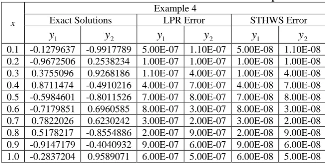
Table 4: Exact Solutions and Error calculation of Example 4
x
Example 4
Exact Solutions LPR Error STHWS Error
1
y
y
2y
1y
2y
1y
2Figure: 1. Error estimation of Example - 1
Figure: 2. Error estimation of Example - 2
Method / IJMA- 4(11), Nov.-2013.
Figure: 4. Error estimation of Example - 3 at
y
2
Figure: 5. Error estimation of Example - 4 at
y
1The above examples 1 to 4 has been solved numerically using the LPR method and STHWS method. The obtained results (with step size time = 0.1) along with exact solutions of the examples 1 to 4 and absolute errors between them are calculated and are presented in Table 1 to 4. A graphical representation is given for the IDEs in Figures 1 to 6, using three-dimensional effect to highlight the efficiency of the STHWS method.
5. CONCLUSIONS
Most integro-differential equations are usually difficult to solve analytically. In many cases, it is required to obtain the approximate solutions. For this purpose, the STHWS Method presented in this paper can be applied. We make use of STHWS method to solve the linear integro-differential equations. From the Tables 1 to 4 and Figures 1 to 6 showed that this method is very convergent for solving linear integro-differential equations. Moreover, the numerical results approximate the exact solution very well. STHWS method can also solve integro-differential equations which can be researched and resolved.
REFERENCES
[1] Asady, B., Kajani, M, T., Direct Method for Solving Integro Differential Equations Using Hybrid Fourier and Block-Pluse Functions, International Journal of Computer Mathematics, 82, 7 (2007), 889-895.
[2] Caglar, H., Caglar, N., Numerical Solution of Integral Equations by Using Local Polynomial Regression, Journal of Computational Analysis and Applications, 10, 2 (2008), 187-195.
[3] Golbabai, A., Javidi, M., Application of He’s Homotopy Perturbation Method for nth-Order Integro-Differential Equations, Applied Mathematics Computation, 190, 2 (2007), 1409-1416.
[4] Han, D. F., Shang, X, F., Numerical Solution of Integro-Differential Equations by Using CAS Wavelet Operational Matrix of Integration, Applied Mathematics Computation, 156, 2 (2007), 460-466.
[5] Jaradat, H., Alsayyed, O., Al-Shara, S., Numerical Solution of Linear Integro-Differential Equations 1, Journal of Mathematics Statistics, 4, 4 (2008), 250-254.
[6] Karamete, A., Sezer, M., A Taylor Collocation Method for the Solution of Linear Integro-Differential Equations, International Journal of Computer Mathematics, 79, 9 (2002), 987-1000.
[7] Liyun Su1, Tianshun Yan, Yanyong Zhao, Fenglan Li, Ruihua Liu, Numerical Solution of Integro-Differential Equations with Local Polynomial Regression, Open Journal of Statistics, 2 (2012), 352-355. [8] Maleknejad, K., Kajani, M. T., Solving linear integro-differential equation system by Galerkin methods
with hybrid functions, Applied Mathematics and Computation, 159 (2004), 603–612.
[9] Pour-Mahmoud, J., Rahimi-Ardabili, M,Y., Shahmorad, S., Numerical Solution of the System of Fredholm Integro-Differential Equations by the Tau Method, Applied Mathematics Computation, 168, 1 (2005), 465-478.
[10] Rashed, M, T., Numerical Solution of Functional Differential, Integral and Integro-Differential Equations, Applied Numerical Mathematics, 156, 2 (2004), 485-492.
[11] Sekar, S., Manonmani, A., A study on time-varying singular nonlinear systems via single-term Haar wavelet series, International Review of Pure and Applied Mathematics, 5(2009), 435-441.
[12] Sekar, S., Balaji, G., Analysis of the differential equations on the sphere using single-term Haar wavelet series, International Journal of Computer, Mathematical Sciences and Applications, 4(2010), 387-393. [13] Sekar, S., Duraisamy, M., A study on CNN based hole-filler template design using single-term Haar wavelet
series, International Journal of Logic Based Intelligent Systems, 4(2010), 17-26.
[14] Sekar, S., Jaganathan, K., Analysis of the singular and stiff delay systems using single-term Haar wavelet series, International Review of Pure and Applied Mathematics, 6(2010), 135-142.
[15] Sekar, S., Kumar, R., Numerical investigation of nonlinear volterra-hammerstein integral equations via single-term Haar wavelet series, International Journal of Current Research, 3(2011), 099-103.
[16] Sekar, S., Paramanathan, E., A study on periodic and oscillatory problems using single-term Haar wavelet series, International Journal of Current Research, 2(2011), 097-105.
[17] Sekar, S., Vijayarakavan, M., Analysis of the non-linear singular systems from fluid dynamics using single-term Haar wavelet series, International Journal of Computer, Mathematical Sciences and Applications, 4(2010), 15-29.
Source of support: Nil, Conflict of interest: None Declared