ISSN 2307-7743 http://scienceasia.asia
MODELING TOBACCO SMOKING EFFECT ON HIV ANTIRETROVIRA THERAPY AND STABILITY ANALYSISL
JACOB ISMAIL IRUNDE, LIVINGSTONE S. LUBOOBI, YAW NKANSAH-GYEKYE
Abstract. Tobacco smoking effect on ARVs remains a topic under investigation. In this paper,
a deterministic model is formulated by considering smoking interference in metabolism of ARVs and its effect on one’s adherence to drugs in order to assess stability of equilibrium states and determine how tobacco smoking affects antiretroviral drugs. Equilibrium states and effective re-production numberRef f are computed and stability condition for equilibrium states established.
Using linearization method and comparison theorem, analysis shows that disease free equilibrium is globally stable whenRef f <1 and it is unstable whenRef f >1. However, due to high smoking
impairment effective reproduction numberRef f cannot be less than unity and the classical
require-mentRef f <1 for global stability of disease free equilibrium cannot be realized. Therefore tobacco
smoking affects stability of disease free equilibrium. By applying logarithmic Lyapunov function, endemic equilibrium is asymptotically stable whenRef f >1. The analysis shows that, as tobacco
smoking interference with metabolism of ARVs increases, HIV infected T-cells and macrophages, and free virus record a corresponding increase and this shows that tobacco smoking decreases the efficacy of ARVs. To improve patient’s immune system and manage HIV epidemic and its therapy, integration of smoking cessation programs in HIV care services is recommended.
1. Introduction
Tobacco smoking remains a top health agenda among HIV infected patients whether they are under therapy or not. Contents of tobacco smoke have a devastating effect in HIV therapy and exacerbate pathogenesis of HIV in the in-vivo dynamics (23). The benefits of ARVs in reducing mortality and suffering among HIV infected individuals are negated by tobacco smoking (5; 19). In addition to causing immune system defective, tobacco smoking also interferes with metabolism of ARVs and causes drug interaction (2). Drug interaction reduces concentration of the drugs’ and cuts down their absorption which entails reduced efficacy.
To gain insight on the effect of tobacco smoking when a HIV smoker is under therapy, we use mathematical modeling to study the behaviour of HIV within a host when ARVs are adminis-tered. Mathematical models play an important role in studying and understanding the dynamics of infectious diseases and their intervention strategies (13). In this study, the model for tobacco
Key words and phrases. Tobacco smoking, antiretroviral therapy, metabolism, stability.
c
smoking effect on antiretroviral therapy is formulated by considering HIV in vivo dynamics and smoking effect on T-cells and macrophages. Stability analysis of the model equilibrium states is performed to determine the qualitative behaviour of the dynamics.
Stability analysis of the model steady states is one of the fundamental problem in mathemati-cal epidemiology (21) as it reveals important features for persistence or eradication of the disease. Understanding of these features which drive a particular disease helps researchers and health prac-titioners to design treatment and intervention strategies (28). Apart from designing treatment and control strategies, stability analysis also offers alert and precautions for disease outbreak.
To perform stability analysis of equilibrium states to determine behaviour of the disease in consid-eration, different approaches have been proposed. However among the approaches, some are useful in analysis of local stability and some for global stability. Linearization method (11; 24) is useful in the analysis of local stability. Under this approach a system is linearized at equilibrium state to obtain a Jacobian matrix. From Jacobian matrix, we compute eigenvalues. If the eigenvalues of the Jacobian matrix are negative or have negative real parts, the equilibrium state is proved stable. However, the equilibrium state is proved unstable when at least one of the eigenvalues is positive or has positive real part.
Sometimes it is difficult to obtain eigenvalues directly from Jacobian matrix. Whenever it is impossible to compute the eigenvalues from the Jacobian matrix, linearization method offers al-ternative methods to test the signs of eigenvalues without computing them. These methods include trace and determinant method, and Hurwitz criterion. Negative trace and positive determinant indicate that, the Jacobian matrix has negative eigenvalues. In Hurwitz criterion, we derive a characteristic equation and test the signs for coefficients. If coefficients do not change sign, nec-essary condition hold. However, sufficient condition depends on the degree of the characteristic equation. Linearization method is also used to analyze local stability of endemic equilibrium.
Comparison theorem (4) and Metzler matrix (12) are used in analysis of global stability of disease free equilibrium. Comparison theorem proves infected classes are diminishing as uninfected classes are growing to attain the disease free equilibrium point. Metzler matrix forms two matrices from uninfected and infected classes. The method concludes global stability if the matrix from unin-fected classes has negative eigenvalues and the elements of the main diagonal in the matrix of the infected classes are negative. However, since global stability implies local stability the approaches may also be used to establish local stability.
equilibrium uses general Lyapunov functions which are reviewed as follows. Explicit Lyapunov function was constructed for the analysis of SEIR and SEIS epidemic models (15; 16). Logarith-mic Lyapunov function was used to analyze Lotka-Voltera systems (6). Later it was used in the analysis of endemic equilibrium for SIR, SIRS and SIS epidemic models (17). Composite qua-dratic Lyaponuv function was proposed and used to determine stability of endemic equilibrium for SIR, SIRS and SIS epidemic models (30). Later the composite-Volterra function was used in the analysis of endemic equilibrium for the model with relapse (30).
As stability is a requirement for the model application in a real setting, this study analyzes stability of a mathematical model for tobacco smoking effect on antiretroviral therapy using lin-earization method, comparison theorem and Lyapunov function. This work is organized as follows: we describe the model in the next Section, analysis of the model is presented after the next Section, Numerical analysis and Conclusion mark the end.
2. Model formulation
The model divides T-cells into five classes and macrophages into four classes. Antiretroviral drugs under consideration are reverse transcription inhibitors (RTIs) and Protease Inhibitors (PIs).
In T-cells, X represents density of uninfected T-cells,X1 density of smoking partially impaired
T-cells, X2 density of HIV latently infected T-cells,X3 density of smoking critically impaired T-cells
and X4 density of HIV productively infected T-cells. For the case of macrophages, Y represents
density of healthy macrophages,Y1 density of smoking partially impaired macrophages, Y2 density
of HIV infected macrophages, Y3 density of smoking critically impaired macrophages and density
of free virus is represented by V.
A function Λ− cV
k+V which decreases due to the presence of free virus (14; 3) is a recruitment
rate for T-cells. The expression γX1 +ηX3 represents smoking T-cells’ impairment rate with
γ < η being relative smoking impairment rates of X1 and X3 due to the fact that, smoking critically impaired T-cells have high concentration of tobacco smoke poisonous and carcinogenic
compounds. Parameters β1, β2 and τ represent HIV infection rates for uninfected T-cells X,
smoking partially impaired T-cells X1 and HIV infection rate of uninfected T-cells X from HIV
infected macrophages Y2 respectively. Since reverse transcription in smoking critically impaired
T-cells X3 is assumed to be spontaneous, in the presence of ARVs, HIV infects smoking critically
impaired T-cells at a rateβ3(1−f1) where such that 0 ≤ ≤1 is the efficacy of RTIs in blocking reverse transcription in T-cells and f1($) =
e−$
$+ 1 is a smoking effect in inducing metabolism
of ARVs in smoking critically impaired T-cells and macrophages, $ ∈ (0,1) is the rate at which
smoking induces metabolism of ARVs. When $ = 0, smoking does not induce metabolism of
Smoking partially impaired T-cells X1 progress to smoking critically impaired T-cells X3 at
a rate ρ. HIV latently infected T-cells X2 due to the presence of smoking partially impaired
T-cells, progress to productively infected T-cells X4 following successful reverse transcription at
a rate σ(1 − f ) where f = e−$ models smoking effect in inducing metabolism of ARVs in
smoking partially impaired T-cells and macrophages. Functions f and f1 model relative smoking
inducing effect in smoking partially and critically impaired cells as we assume smoking critically impaired cells experience high smoking inducing effect compared to smoking partially impaired
cells. However, if ζ1 denotes drugs’ reverse transcription blocking rate in T-cells and ϑ adherence
rate to treatment, then =ζ1ϑ. Parameter α is smoking induced mortality in critically impaired
T-cells and µ1 is a HIV induced mortality in HIV productively infected T-cells which produce
infectious virions at a rate N1µ1(1−f1ξ). The parameter ξ = κϑ such that 0 ≤ ξ ≤ 1 is the
efficacy of PIs in blocking production of infectious virions in T-cells, κ is the rate at which PIs
block production of infectious virions in T-cells and ϑ is drugs’ adherence rate.
Macrophages are recruited at a rate λ. Expressions β4(1−1), β5(1−f 1) andβ6(1−f11) are
HIV infection rates for healthy macrophages Y, smoking partially impaired macrophages Y1 and
smoking critically impaired macrophages Y3, where1 =ζ2ϑ such that 0≤1 ≤1 is the efficacy of
RTIs in macrophages and ζ2 is the rate at which RTIs block reverse transcription in macrophages.
Expression νY1+θY3 is a smoking impairment rate with relative impairment of Y1 and Y3 given
by ν and θ, we assume that ν < θ because smoking critically impaired macrophages have high
concentration of tobacco smoke poisonous and carcinogenic compounds. Smoking critically
im-paired macrophages suffer smoking induced mortality at a rate α1. HIV infected macrophages
suffer HIV induced mortality at rate δ and produce infectious virions at a rate N2δ(1−f1ξ1)
where ξ1 = κ1ϑ such that 0 ≤ ξ1 ≤ 1 is the efficacy of PIs in blocking production of infectious
virions in macrophages and κ1 is the rate at which PIs’ block production of infectious virions.
Parametersµy andµv represent natural mortalities for macrophages’ compartments and free virus
respectively.
X
X 4 X
3
X 2 X
1
Y 3 Y
2
Y 1 Y
Λ−cV/(k+V)
(γX
1+ηX3)X β
1VX+τY2X µX
β 2VX1
ρX 1
σ(1−fε)X 2 µX
1 µX2
β3(1−f 1ε)VX3
(µ+α)X 3
(µ+µ 1)X4
λ
(νY
1+θY3)Y β4(1−ε
1)VY
β
5(1−fε1)VY1 µ
yY
qY 1 β6(1−f
1ε1)VY3
µ yY1 (µ
y+δ)Y2
(µ y+α1)Y3
V a(1−sξ)X
4+b(1−sξ1)Y2
µvV (β
1X+β2X1+β3(1−f1ε)X3)V (β4(1−ε1)Y+β5φ1Y1+β6φ2Y3)V CD4+
T−cells
Macrophages
Figure 2.1. Interaction of T-cells and macrophages with free virus and tobacco
smoking in the presence of therapy.
Table 2.1. Variables description
Variable Description
X Uninfected CD4+ T-cells
X1 Smoking partially impaired CD4+ T-cells
X2 HIV latently infected CD4+ T-cells
X3 Smoking critically impaired CD4+ T-cells
X4 HIV productively infected CD4+ T-cells
Y Healthy macrophages
Y1 smoking partially impaired macrophages
Y2 HIV infected macrophages
Y3 Smoking critically impaired macrophages
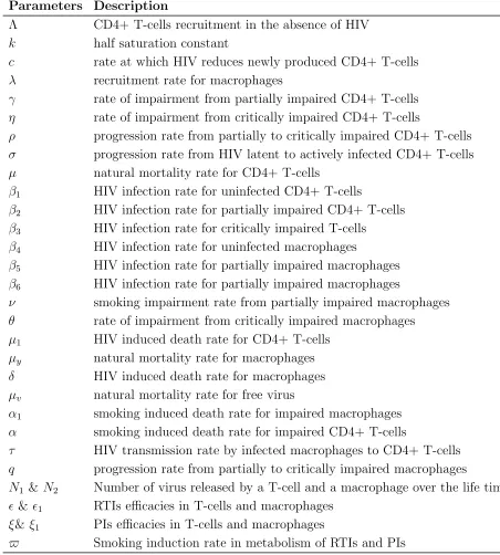
Table 2.2: Parameters descriptions
Parameters Description
Λ CD4+ T-cells recruitment in the absence of HIV
k half saturation constant
c rate at which HIV reduces newly produced CD4+ T-cells
λ recruitment rate for macrophages
γ rate of impairment from partially impaired CD4+ T-cells
η rate of impairment from critically impaired CD4+ T-cells
ρ progression rate from partially to critically impaired CD4+ T-cells
σ progression rate from HIV latent to actively infected CD4+ T-cells
µ natural mortality rate for CD4+ T-cells
β1 HIV infection rate for uninfected CD4+ T-cells
β2 HIV infection rate for partially impaired CD4+ T-cells
β3 HIV infection rate for critically impaired T-cells
β4 HIV infection rate for uninfected macrophages
β5 HIV infection rate for partially impaired macrophages
β6 HIV infection rate for partially impaired macrophages
ν smoking impairment rate from partially impaired macrophages
θ rate of impairment from critically impaired macrophages
µ1 HIV induced death rate for CD4+ T-cells
µy natural mortality rate for macrophages
δ HIV induced death rate for macrophages
µv natural mortality rate for free virus
α1 smoking induced death rate for impaired macrophages
α smoking induced death rate for impaired CD4+ T-cells
τ HIV transmission rate by infected macrophages to CD4+ T-cells
q progression rate from partially to critically impaired macrophages
N1 &N2 Number of virus released by a T-cell and a macrophage over the life time
&1 RTIs efficacies in T-cells and macrophages
ξ& ξ1 PIs efficacies in T-cells and macrophages
From the flow diagram 2.1, the model is governed by the following system of differential equations:
dX
dt = Λ− cV
k+V −(γX1 +ηX3)X−β1V X−τ Y2X−µX,
(1a)
dX1
dt = (γX1+ηX3)X−β2V X1−(ρ+µ)X1,
(1b)
dX2
dt =β1V X+τ Y2X+β2V X1−(σ(1−f ) +µ)X2,
(1c)
dX3
dt =ρX1−β3(1−f1)V X3 −(α+µ)X3,
(1d)
dX4
dt =σ(1−f )X2+β3(1−f1)V X3−(µ1+µ)X4,
(1e)
dY
dt =λ−β4(1−1)V Y −(νY1+θY3)Y −µyY,
(1f)
dY1
dt = (νY1+θY3)Y −β5(1−f 1)V Y1−(q+µy)Y1,
(1g)
dY2
dt =β4(1−1)V Y +β5(1−f 1)V Y1+β6(1−f11)V Y3−(δ+µy)Y2,
(1h)
dY3
dt =qY1 −β6(1−f11)V Y3−(α1+µy)Y3,
(1i)
dV
dt =N1µ1(1−f1ξ)X4+N2δ(1−f1ξ1)Y2−β1V X−β2V X1−β3(1−f1)V X3
−β4(1−1)V Y −β5(1−f 1)V Y1−β6(1−f11)V Y3−µvV, (1j)
subject to initial conditions X(0) = X0, X1(0) = X10, X2(0) = 0, X3(0) = 0, X4(0) = 0,
Y(0) = Y0, Y1(0) =Y10, Y2(0) = 0, Y3(0) = 0, and V(0) =V0.
3. Model Analysis
In this section the region under which the solutions of model (1) are bounded is deduced and we compute equilibrium states, effective reproduction number and determine condition for equilibria stability.
3.1. Boundedness of Solutions.
To prove boundedness of solutions we consider T-cells, macrophages and free virus separately.
If Tt represents sum of T-cells in all compartments, we have:
dTt
dt = Λ−
cV
k+V −µTt−αX3−µ1X4,
dTt
Rearrangement gives the following equation:
(2) dTt
dt +µTt≤Λ
whose general solution is given by
(3) Tt ≤
Λ
µ +
Tt(0)− Λ
µ
e−µt.
Considering the two cases when Tt(0)> Λ
µ and when Tt(0) <
Λ
µ, we have:
(4)
Tt ≤Φt, where
Φt=max
Tt(0),
Λ
µ
.
However, since Tt represents the sum of all T-cells, it follows that:
(5) X4 ≤Φt.
For the case of macrophages if Mtrepresents the sum of macrophages in all compartments and we
apply the same procedures as for T-cells, we have
(6) Mt ≤Φm =max
Mt(0),
λ µy
.
Since Mt is the sum of macrophages in all compartments, it follows that
(7) Y2 ≤Φm.
We now consider equation (1j), so that
dV
dt =N1µ1(1−f1ξ)X4+N2δ(1−f1ξ1)Y2−β1V X−β2V X1−β3(1−f1)V X3
−β4(1−1)V Y −β5(1−f 1)V Y1−β6(1−f11)V Y3−µvV,
dV
dt ≤N1µ1(1−f1ξ)X4+N2δ(1−f1ξ1)Y2−µvV.
Substitution of X4 and Y2 in equation
(8) dV
dt ≤N1µ1(1−f1ξ)X4+N2δ(1−f1ξ1)Y2−µvV,
yields solution which shows that free virus are also bounded. The solution is given by
(9) V(t)≤Ψ01,
where
Ψ01 =M ax
N1µ1(1−f1ξ)Tt(0)
µv
+N2δ(1−f1ξ1)Mt(0)
µv
,N1µ1(1−f1ξ)Λ µµv
+ N2δ(1−f1ξ1)λ
µyµv
.
The solutions of the model system are bounded in the region
(10) Υ =(T, Y, M, V)∈R10
where T and M represent T-cells’ and macrophages’ compartments respectively.
Any solution on the boundary of Υ converges and remains in the region. Existence, uniqueness and continuity of solutions of the model (1) hold in Υ.
3.2. Disease Free Equilibrium and Effective Reproduction Number Ref f.
The disease free equilibrium of the model (1) when there is no tobacco smoking and HIV is given by
(11) χ0(X, X1, X2, X3, X4, Y, Y1, Y2, Y3, V) =
Λ
µ,0,0,0,0, λ µy
,0,0,0,0
We use disease free equilibrium to compute effective reproduction numberRef f in the next section.
3.2.1. Effective Reproduction Number Rf f. If we consider the infected classes in a model system
(1) so that the new infections and transfer terms are defined byMi andNi respectively, the matrix
M and N are defined by
(12) M= ∂Mi
∂Xj
(χ0) and N= ∂Ni
∂Xj (χ0).
According to (29), the effective reproduction number Ref f is given by
(13) Ref f =ρ MN−1
which is the maximum eigenvalue of the matrix MN−1. From the model (1), we define the new
infections and transfer terms to be
(14) Mi =
(γX1+ηX3)X
β1V X+τ Y2X+β2V X1 0
β3(1−f1)V X3 (νY1+θY3)Y
β4(1−1)V Y +β5(1−f 1)V Y1+β6(1−f11)V Y3 0
N1µ1(1−f1ξ)X4+N2δ(1−f1ξ1Y2
and
(15) Ni =
(ρ+µ)X1 (σ(1−f ) +µ)X2
(α+µ)X3−ρX1 (µ1+µ)X4 −σ(1−f )X2
(q+µy)Y1 (δ+µy)Y2 (α1+µy)Y3−qY1
µvV
From equation (13), the effective reproduction number Ref f works out to be:
(16) Ref f =max{Ref f1, Ref f2}
where
Ref f1 =
Λγ µ(ρ+µ)+
Ληρ
µ(ρ+µ)(α+µ),
Ref f2 =
λν µy(q+µy)
+ λνq
µy(q+µy)(α1+µy)
.
The effective reproduction number Ref f is given as the maximum of partial effective reproductive
number due to tobacco smoking in T-cells Rf f1 and partial effective reproductive number due to
tobacco smoking in macrophages Rf f2. Tobacco smoking dominates HIV in producing new
infec-tions. The partial effective reproductive numbers Rf f1 and Rf f2 can be written as the sum of new
infections which are caused by smoking partially impaired cells and those caused by smoking crit-ically impaired cells. If the new infections which are caused by smoking partially impaired T-cells
are defined by ReP T and those caused by smoking critically impaired T-cells by ReCT then
(17)
Ref f1 =ReP T +ReCT,
where ReP T =
Λγ
µ(ρ+µ) and ReCT =
Ληρ
µ(ρ+µ)(α+µ).
Similarly for the case of macrophages, if the new infections which are caused by smoking
par-tially impaired macrophages are defined by ReP M and those which are caused by smoking critically
impaired macrophages by ReCM then
(18)
Ref f2 =ReP M +ReCM, where
ReP M =
λν µy(q+µy)
and ReCM =
λνq
µy(q+µy)(α1 +µy)
.
We use effective reproduction number Ref f to determine stability of disease free equilibrium.
3.2.2. Local stability of a Disease Free Equilibrium χ0. When tobacco smoking impairs less than
one cell (T-cells or macrophages) and HIV infects less than one cell (T-cells or macrophages) a
case in whichRef f <1, disease free equilibrium is locally asymptotically stable. It becomes unstable
when tobacco smoking impairs more than one cell (T-cells or macrophages) and HIV infects more
than one cell (T-cells or macrophages) the case in which Ref f > 1. To find condition for local
stability of disease free equilibrium, we state and prove the following theorem.
To prove the theorem, we linearize the model system (1) at disease free equilibrium to obtain a matrix
(19) J(χ0) =
−µ −γΛ
µ 0 −
γη
µ 0 0 0 −
τΛ
µ 0 −
c k −
β1Λ µ 0 γΛ
µ −w1 0
ηΛ
µ 0 0 0 0 0 0
0 0 −wA 0 0 0 0
τΛ
µ 0
β1Λ µ
0 ρ 0 −w0 0 0 0 0 0 0
0 0 σ(1−f ) 0 −w6 0 0 0 0 0
0 0 0 0 0 −µy −
νλ µy
0 −θλ
µy
−d3
µy
0 0 0 0 0 0 νλ
µy
−w3 0 θλ
µy
0
0 0 0 0 0 0 0 −w4 0 d3
µy
0 0 0 0 0 0 q 0 −w2 0
0 0 0 0 d1 0 0 d2 0 −β1Λ
µ − d3 µy
−µv
where
d1 =N1µ1(1−f1ξ), d2 =N2δ(1−f1ξ1), d3 =β4λ(1−1).
Negative eigenvalues from matrix J(χ0) will mean stable disease free equilibrium. Negative trace
and positive determinant of the matrix J(χ0) also means that the eigenvalues of the matrix J(χ0)
are negative and disease free equilibrium is stable. After identifying two negative eigenvalues −µ
and −µy in first and sixth columns, the matrix reduces to
(20) J1(χ0) =
γΛ
µ −w1 0
ηΛ
µ 0 0 0 0 0
0 −wA 0 0 0
τΛ
µ 0
β1Λ µ
ρ 0 −w0 0 0 0 0 0
0 σ(1−f ) 0 −w6 0 0 0 0
0 0 0 0 νλ µy
−w3 0 θλ
µy
0
0 0 0 0 0 −w4 0 d3 µy
0 0 0 0 q 0 −w2 0
0 0 0 d1 0 d2 0 −β1Λ
µ − d3 µy
−µv
If we denote trace and determinant of matrix J1(χ0) bytrJ1 anddetJ1, then trace and
determi-nant are given by
(21) trJ1 =w1(ReP T −1) +w3(ReM P −1)−
β1Λ
µ −
β4(1−1)
µy
−µv−w0−w2
and
(22)
detJ1 = Φ
β1Λ
µµv
+β4(1−1)λ
µyµv
+ 1−ReH
(1−Ref f1)(1−Ref f2),
where ReH =
(τ β4(1−1) +β1µµyw4)σΛN1µ1(1−f1ξ)(1−f )
µµyµvwAw4w6
+N2δ(1−f1ξ1)β4(1−1)λ
µyµvw4
, Φ =µvwAw0w1w2w3w4w6.
The expressions for ReP T and ReM P are given in (17) and (18) respectively. We find that
(23) trJ1 <0 if and only if ReP T <1 and ReM P <1,
and
(24)
detJ1 >0 if and only if Ref f1 <1, Ref f2 <1 and ReH <
β1Λ
µµv
+β4(1−1)λ
µyµv
+ 1.
Non-negative determinant and negative trace represent a model system with locally asymptotically
stable disease fee equilibrium when Ref f < 1. However since Ref f is the maximum of Ref f1 and
Ref f2, stable disease free equilibrium will not be realized when Ref f1 >1 and Ref f2 >1.
3.2.3. Global Stability of a Disease Free Equilibrium χ0. Global stability analysis of a disease free equilibrium is usually done by Lyaponuv functions as applied in (27), (31), (25) and (26), and by comparison theorem as used in (4; 9) and (32). Since Lyapunov functions are not unique and present a challenge in construction, this work adopts comparison theorem in global stability anal-ysis for disease free equilibrium.
Considering infected classes alone in the model (1), we write the system without uninfected
(25)
X10 X20 X30 X40 Y10 Y20 Y30 V0
= (M−N)
X1 X2 X3 X4 Y1 Y2 Y3 V −
(γX1+ηX3)
Λ
µ −X
(τ Y2+β1V)
Λ
µ −X
0 0
(νY1+θY3)
λ µy
−Y
β4V
λ µy −Y 0
L+β1V
X− Λ
µ
+β4(1−1)V
Y − λ
µy
L=β1V Λ
µ +β4(1−1)V λ µy
+β2V X1+β3(1−f1)V X3+β5(1−f 1)V Y1+β6V(1−f11)Y3.
Matrices M and N represent new infections and transfer terms respectively. For t > 0, X ≤ Λ
µ
and Y ≤ λ
µy
we see that
(26)
X10 X20 X30 X40 Y10 Y20 Y30 V0
≤(M−N)
X1 X2 X3 X4 Y1 Y2 Y3 V
Since the matrix M−N has negative eigenvalues, equation (26) represents a stable disease free
equilibrium whereby (X, Y) →
Λ µ, λ µy
and (X1, X2, X3, X4, Y1, Y2, Y3, V) → (0,0,0,0,0,0,0,0)
as t → ∞. This shows that a disease free equilibrium is globally asymptotically stable. We
summarize this result in Theorem 2.
Theorem 2. : The disease equilibrium χ0 is globally asymptotically stable when (X, Y) →
Λ µ, λ µy
and (X1, X2, X3, X4, Y1, Y2, Y3, V)→(0,0,0,0,0,0,0,0) for which Ref f <1
3.2.4. Global stability of endemic equilibrium. By reverse condition as stated by (29) the endemic
equilibrium Υ∗ is locally stable. Lyapunov functions and LaSalle invariant principle are used to
Lyapunov function by
(27) U2(T, M, V) =b(T −T∗lnT) +c(M −M∗lnM) +d(V −V∗lnV),
T, M and V represent T-cells, macrophages and free virus respectively and T∗, M∗ and V∗
represent T-cells, macrophages and free virus at endemic equilibrium point. In full, function
U2(T, M, V) is written as
(28)
U2(T, M, V) = b1(X−X∗lnX) +b2(X1−X1∗lnX1) +b3(X2−X2∗lnX2) +b4(X3−X3∗lnX3) +b5(X4−X4∗lnX4) +b6(Y −Y∗lnY) +b7(Y1−Y1∗lnY1) +b8(Y2 −Y2∗lnY2) +b9(Y3−Y3∗lnY3) +b10(V −V∗lnV).
Derivative of equation (28) with respect to time, gives
(29)
dU2
dt =b1
1− X
∗
X
dX dt +b2
1−X
∗ 1
X1
dX1
dt +b3
1− X
∗ 2 X2 dX2 dt
+b4
1− X
∗ 3
X3
dX3
dt +b5
1− X
∗ 4
X4
dX4
dt +b6
1−Y
∗
Y
dY dt
+b7
1− Y
∗ 1
Y1
dY1
dt +b8
1− Y
∗ 2
Y2
dY2
dt +b9
1− Y
∗ 3 Y3 dY3 dt
+b10(1−
V∗ V )
V dt,
Substitution of the rate of change for each variable at endemic equilibrium, simplification and rearrangements give
(30)
dU2
dt =−b1µX
1−X
∗
X 2
−b2w1X1
1− X
∗ 1
X1
2
−b3wAX2
1− X
∗ 2
X2
2
−b4w0X3
1−X
∗ 3
X3
2
−b5w6X4
1− X
∗ 4
X4
2
−b6µyY
1−Y
∗
Y 2
−b7w3Y1
1− Y
∗ 1
Y1
2
−b8w4Y2
1−Y
∗ 2
Y2
2
−b9w2Y3
1− Y
∗ 3
Y3
2
−b10µvV
1−V
∗
V 2
where
(31)
F2 =−b1γXX1
1− X
∗
X 1−
X∗X1∗ XX1
−b1ηXX3
1− X
∗
X 1−
X∗X3∗ XX3
−b1β1V X
1−X
∗
X 1−
V∗X∗ V X
−b1τ Y2X
1−X
∗
X 1−
Y2∗X∗ Y2X
−b2β2V X1
1− X
∗ 1
X1
1− V
∗X∗
1
V X
−b4β3(1−f1)V X3
1− X
∗ 3
X3
1− V
∗X∗
3
V X3
−b6β4(1−1)V Y
1− Y
∗
Y 1−
V∗Y∗ V Y
−b6νY Y1
1− Y
∗
Y 1−
Y∗Y1∗ Y Y1
−b6θY Y3
1− Y
∗
Y 1−
Y∗Y3∗ Y Y3
−b7β5(1−f 1)V Y1
1− Y
∗ 1
Y1
1− V
∗Y∗
1
V Y1
−b9β6(1−f11)V Y3
1− Y
∗ 3
Y3
1− V
∗Y∗
3
V Y3
−b10β1V X
1− V
∗
V 1−
V∗X∗ V X
−b10β2V X1
1−V
∗
V 1−
V∗X1∗ V X1
−b10β3V X3
1− V
∗
V 1−
V∗X3∗ V X3
−b10β4V Y
1− V
∗
V 1−
V∗Y∗ V Y
−b10β5V Y1
1− V
∗
V 1−
V∗Y1∗ V Y1
−b10β6V Y3
1− V
∗
V 1−
V∗Y3∗ V Y3
.
Following the approach in (22) and (20), F2 is non-positive. Function
F2 ≤0 for X, X1, X2, X3, X4, Y, Y1, Y2, Y3, V >0. The time derivative
dU2
dt ≤0 when
X, X1, X2, X3, X4, Y, Y1, Y2, Y3, V > 0, for X = X∗, X1 = X1∗, X2 = X2∗, X3 = X3∗, X4 = X4∗,
Y =Y∗, Y1 =Y1∗, Y2 =Y2∗, Y3 =Y3∗, V =V
∗, dU2
dt = 0. This indicates that, the largest invariant
set Υfor which dU2
dt = 0 is a singleton Υ
∗ which is endemic equilibrium. Using LaSalle Invariant
Principle (18), Υ∗ is globally stable in the interior ofΥ whenRef f >1. This result is summarized
in the following theorem
Theorem 3. : If Ref f >1, then the model system (1) has unique endemic equilibrium Υ∗ which
is globally asymptotically stable in the interior of Υ∗.
4. Numerical Analysis
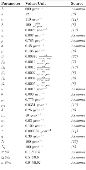
Table 4.1: Parameter values
Parameter Value/Unit Source
Λ 600 year−1 Assumed
k 12 (3)
c 110 year−1 (14)
λ 100 ml yaercells (8)
γ 0.0025 year−1 (10)
η 0.007 year−1 Assumed
ρ 0.785 year−1 Assumed
σ 0.45 year−1 Assumed
µ 0.135 year−1 (8)
β1 0.00876 virus yearml (26)
β2 0.0012 virus yearml (7)
β3 0.0016 virus yearml (10)
β4 0.0002 virus yearml (8)
β5 0.0004 virus yearml (8)
β6 0.0005 virus yearml (8)
ν 0.0016 year−1 Assumed
θ 0.003 year−1 Assumed
µ1 0.775 year−1 Assumed
µy 0.0351 year−1 (10)
δ 0.25 year−1 (8)
µv 50 year−1 Assumed
α1 0.03 year−1 Assumed
α 0.102 year−1 Assumed
τ 0.000365 year−1 (14)
q 0.38 year−1 Assumed
N1 100 year−1 (26)
N2 100 year−1 (8)
$&ϑ 0.1 & 0.5 Assumed
ζ1&ζ2 0.5 &0.6 Assumed
κ1&κ2 0.9 &0.92 Assumed
In this section, we begin by plotting the general dynamics for model (1). Figure 4.1 shows the
at a rate 0.3. The dynamics show the existence of unstable disease free equilibrium between 0
and 2 years. During this time interval, uninfected T-cells and healthy macrophages grow slightly.
However, smoking compartments indicate a fast growth compared to HIV compartments which take over later.
0 5 10 15 20 25
0 100 200 300 400 500 600 700 800
Time[years]
T−cells, macrophages and virus Populations (cells/mm
3)
X X1 X2 X3 X4 Y Y1 Y2 Y3 V
0 5 10 15 20 25
0 100 200 300 400 500 600
Time[years]
Uninfected T−cells and healthy macrophages (cells/mm
3)
Figure 4.1. Variation of cells’ populations in the general dynamics when a HIV
smoker is under therapy.
To show the endemic equilibrium, we plot HIV infected and smoking impaired classes and they
are shown in Figure 4.2. Smoking impaired classes increase between 0 and 5 years and on their
downfall HIV infected classes and free virus increases.
0 5 10 15 20 25
0 100 200 300 400 500 600 700
Time[days]
Smoking impaired classes(cells/mm
3)
X1
X
3
Y
1
Y3
0 5 10 15 20 25
0 100 200 300 400 500 600 700 800
Time[years]
HIV infected classes and free virus (cells/mm
3)
X
2
X4
Y
2
V
Figure 4.2. Variation of HIV infected and smoking impaired classes with time.
ARVs.
In Figures 4.3 and 4.4, HIV actively infected T-cells, HIV infected macrophages and free virus increase correspondingly with increasing in interference of ARVs’ metabolism. This shows that smoking interference in metabolism of ARVs reduces drugs’ efficacy. For HIV latently infected
T-cells as antiretroviral drugs are taken, they increase from 0 to10 years. However from 10years
and above HIV latently infected T-cells decreases as smoking interference with metabolism of ARVs increases. This is the time when ARVs becomes ineffective due to tobacco smoking.
0 5 10 15 20
0 100 200 300 400 500 600 700 800 900 1000
Time[years]
HIV latently infected T−cells (cells/mm
3)
ϖ=0.1 ϖ=0.3 ϖ=0.5 ϖ=0.7
0 5 10 15 20
0 50 100 150 200 250 300 350 400 450 500
Time[years]
HIV actively infected T−cells (cells/mm
3)
ϖ=0.1 ϖ=0.3 ϖ=0.5 ϖ=0.7
Figure 4.3. Variation of HIV actively and latently infected T-cells with respect to
smoking inducing effect.
0 5 10 15 20
0 100 200 300 400 500 600 700
Time[years]
HIV infected Macrophages (cells/mm
3)
ϖ=0.1 ϖ=0.3 ϖ=0.5 ϖ=0.7
0 5 10 15 20
0 100 200 300 400 500 600 700 800 900
Time[years]
Free virus (virus/mm
3)
ϖ=0.1 ϖ=0.3 ϖ=0.5 ϖ=0.7
Figure 4.4. Variation of HIV infected macrophages and free virus with respect to
smoking inducing effect.
already established earlier. Convergence for trajectories indicates that endemic equilibrium exists, and it is globally asymptotically stable whenever it exists.
0 5 10 15 20
0 100 200 300 400 500 600
Time[years]
Uninfected T−cells (cells/mm
3)
0 5 10 15 20
0 50 100 150 200 250
Time[years]
Healthy macrophages (cells/mm
3)
Figure 4.5. Trajectories of uninfected T-cells and healthy macrophages.
0 5 10 15 20
0 100 200 300 400 500 600 700 800 900 1000
Time[years]
Smoking critically impaired T−cells (cells/mm
3)
0 5 10 15 20
0 50 100 150 200 250 300 350 400
Time[years]
Smoking critically impaired macrophages (cells/mm
3)
Figure 4.6. Trajectories of Smoking critically impaired T-cells and macrophages.
0 5 10 15 20
0 50 100 150 200 250 300 350 400 450 500
Time[years]
HIV actively infected T−cells (cells/mm
3)
0 5 10 15 20
0 100 200 300 400 500 600
Time[years]
HIV infected macrophages (cells/mm
Figure 4.7. Trajectories of HIV actively infected T-cells and macrophages.
0 2 4 6 8 10 12 14 16 18 20
0 100 200 300 400 500 600 700 800
Time[years]
Free virus (virus/mm
3
)
Figure 4.8. Trajectories of free virus.
5. Conclusion
A mathematical model to determine the effect of tobacco smoking on antiretroviral therapy and assess stability of equilibrium states is presented and analyzed. The effective reproduction number
Ref f is computed by using next generation approach (29) and it is given as the maximum of partial
effective reproduction numbers due to tobacco smoking in T-cellsRef f1 and macrophagesRef f2. The
disease free equilibrium is shown to be globally asymptotically stable when Ref f <1. However with
the parameters that we have used in simulation, Ref f1 and Ref f2 are not less than unit. SinceRef f
is the maximum of Ref f1 and Ref f2, it will never be less than unity and the classical requirement
of Ref f < 1 for global stability of disease free equilibrium cannot be achieved. Therefore tobacco
smoking affects stability of disease free equilibrium.
Numerical simulation indicates that the unstable disease free equilibrium and stable endemic equilibrium exist. Convergence of trajectories in Figures 4.5, 4.6, 4.7 and 4.8 proves the existence of endemic equilibrium and its stability. Endemic equilibrium is asymptotically stable whenever it
exists when Ref f >1. Simulation indicates that tobacco smoking reduces the efficacy of
antiretro-viral therapy. This is reflected by increase of free virus, HIV infected T-cells and macrophages when smoking induces metabolism of ARVs.
Conflict of interest
The authors thank Mkwawa University College of Education and Nelson Mandela African Insti-tution of Science and Technology for the support. However, the conclusion made in this study is not influenced by any institution.
References
.
[1] B. Adams, H. Banks, M. Davidian, H.-D. Kwon, H. Tran, S. Wynne, and
E. Rosenberg, Hiv dynamics: modeling, data analysis, and optimal treatment protocols,
Journal of Computational and Applied Mathematics, 184 (2005), pp. 10–49.
[2] A. Ande, C. McArthur, A. Kumar, and S. Kumar, Tobacco smoking effect on
hiv-1 pathogenesis: role of cytochrome p450 isozymes, Expert opinion on drug metabolism & toxicology, 9 (2013), pp. 1453–1464.
[3] P. Das, D. Mukherjee, A. Sen, Z. Mukandavire, and C. Chiyaka, Analysis of an
in-host model for HIV dynamics with saturation effect and discrete time delay, Nonlinear Dynamics and Systems Theory, 11 (2011), pp. 125–136.
[4] O. Diekmann, J. A. P. Heesterbeek, and J. A. Metz, On the definition and the com-putation of the basic reproduction ratio R0 in models for infectious diseases in heterogeneous populations, Journal of mathematical biology, 28 (1990), pp. 365–382.
[5] J. G. Feldman, H. Minkoff, M. F. Schneider, S. J. Gange, M. Cohen, D. H.
Watts, M. Gandhi, R. S. Mocharnuk, and K. Anastos, Association of cigarette
smoking with HIV prognosis among women in the HAART era: a report from the women’s interagency HIV study, American Journal of public health, 96 (2006), pp. 1060–1065. [6] B. Goh, Management and analysis of biological Populations, Armsterdam, 1980.
[7] M. Hadjiandreou, R. Conejeros, and V. S. Vassiliadis, Towards a long-term model construction for the dynamic simulation of HIV infection., Mathematical biosciences and engineering: MBE, 4 (2007), pp. 489–504.
[8] E. A. Hernandez-Vargas and R. H. Middleton, Modeling the three stages in HIV
infection, Journal of theoretical biology, 320 (2013), pp. 33–40.
[9] M. Imran, M. Hassan, M. Dur-E-Ahmad, and A. Khan, A comparison of a
deter-ministic and stochastic model for hepatitis c with an isolation stage, Journal of biological dynamics, 7 (2013), pp. 276–301.
[10] J. I. Irunde, L. S. Luboobi, and Y. Nkansah-Gyekye, Modeling the effect of tobacco
smoking on the in-host dynamics of HIV/AIDS, Journal of Mathematical and Computational Science, 6 (2016), pp. 1–31.
[11] R. A. Jamal, A. Chow, and K. Morris, Linearized stability analysis of nonlinear partial differential equations, arXiv preprint arXiv:1509.05792, (2015).
[12] J. C. Kamgang and G. Sallet, Computation of threshold conditions for epidemiological models and global stability of the disease-free equilibrium (DFE), Mathematical biosciences, 213 (2008), pp. 1–12.
[13] M. A. Khan, Z. Ali, L. Dennis, I. Khan, S. Islam, M. Ullah, and T. Gul,
Sta-bility analysis of an svir epidemic model with non-linear saturated incidence rate, Applied Mathematical Sciences, 9 (2015), pp. 1145–1158.
[14] D. E. Kirschner and G. F. Webb, A mathematical model of combined drug therapy of
HIV infection, Computational and Mathematical Methods in Medicine, 1 (1997), pp. 25–34. [15] A. Korobeinikov, Lyapunov functions and global properties for seir and seis epidemic
models, Mathematical Medicine and Biology, 21 (2004), pp. 75–83.
[16] , Global properties of infectious disease models with nonlinear incidence, Bulletin of
Mathematical Biology, 69 (2007), pp. 1871–1886.
[17] A. Korobeinikov and G. C. Wake, Lyapunov functions and global stability for sir, sirs,
and sis epidemiological models, Applied Mathematics Letters, 15 (2002), pp. 955–960. [18] J. P. LaSalle, The stability of dynamical systems, vol. 25, SIAM, 1976.
[19] A. R. Lifson, J. Neuhaus, J. R. Arribas, M. van den Berg-Wolf, A. M. Labriola,
and T. R. Read, Smoking-related health risks among persons with hiv in the strategies for
management of antiretroviral therapy clinical trial, American journal of public health, 100 (2010), pp. 1896–1903.
[20] C. C. McCluskey, Lyapunov functions for tuberculosis models with fast and slow
progres-sion, Mathematical Biosciences and Engineering, (2006), pp. 603–604.
[21] S. C. Mpeshe, L. S. Luboobi, and Y. Nkansah-Gyekye, Stability analysis of the rift
valley fever dynamical model, Journal of Mathematical and Computational Science, 4 (2014), pp. 1–23.
[22] Z. Mukandavire, W. Garira, and J. Tchuenche, Modelling effects of public health
educational campaigns on hiv/aids transmission dynamics, Applied Mathematical Modelling, 33 (2009), pp. 2084–2095.
[23] P. Rao and S. Kumar, Polycyclic aromatic hydrocarbons and cytochrome p450 in hiv pathogenesis., Frontiers in microbiology, 6 (2014), pp. 550–550.
[24] M. R. Roussel, Stability analysis for ODEs, Nonlinear Dynamics, lecture notes, (2005).
[25] H. L. Smith, L. Wang, and M. Y. Li, Global dynamics of an seir epidemic model with
vertical transmission, SIAM Journal on Applied Mathematics, 62 (2001), pp. 58–69.
[26] P. Srivastava, M. Banerjee, and P. Chandra, Modeling the drug therapy for HIV
infection, Journal of Biological Systems, 17 (2009), pp. 213–223.
[27] P. K. Srivastava and P. Chandra, Modeling the dynamics of hiv and CD4+ T cells
during primary infection, Nonlinear Analysis: Real World Applications, 11 (2010), pp. 612– 618.
[29] P. Van den Driessche and J. Watmough, Reproduction numbers and sub-threshold en-demic equilibria for compartmental models of disease transmission, Mathematical biosciences, 180 (2002), pp. 29–48.
[30] C. Vargas-De-Le´on, On the global stability of infectious diseases models with relapse,
Abstraction and Application Magazine, 9 (2014).
[31] L. Wang and M. Y. Li, Mathematical analysis of the global dynamics of a model for hiv
infection of cd4+ t cells, Mathematical Biosciences, 200 (2006), pp. 44–57.
[32] T. Zhang and Z. Teng, Pulse vaccination delayed seirs epidemic model with saturation
incidence, Applied Mathematical Modelling, 32 (2008), pp. 1403–1416.
Jacob Ismail Irunde, Nelson Mandela African Institution of Science and Technology, Tanzania
Livingstone S. Luboobi, Makerere University, Box 7062, Kampala, Uganda