Vol 7, No 7 (2017)

(1)

Research Article

July

2017

Computer Science and Software Engineering

ISSN: 2277-128X (Volume-7, Issue-7)

Modeling on Eco-System Consisting of Two Hosts-One Commensal

with Mortality Rates for the Second and Third Species

B. Hari Prasad, Dr. M. Sunder Ram

Department of Mathematics, Chaitanya Group of Colleges, Hanamkonda, T.S, India

DOI:10.23956/ijarcsse/V7I7/0198

Abstract- In this paper, the system comprises of two hosts S1, S2 and one commensal S3 ie., S1 and S2 both benefit S3,

without getting themselves affected either positively or adversely. Further, S1 and S2 are neutral. Here all the three

species posses limited resources. The model equations constitute a set of three first order non-linear simultaneous differential equations. Criteria for the asymptotic stability of all the eight equilibrium states are established. The system would be stable if all the characteristic roots are negative, in case they are real, and have negative real parts, in case they are complex. The global stability of the system is established with the aid of suitably constructed Liapunov’s functions and the numerical solutions for the growth rate equations are computed using Runge-Kutta fourth order scheme.

Keywords— Asymptotically stable, Commensal, Equilibrium state, Host, Trajectories, Stable, Unstable.

I. INTRODUCTION

Ecology is a branch of life and environment sciences which asserts the existence of diverse species in the same environment and habitat. It is a common observation that the species of the same nature can not flourish in isolation without any interaction with species of different kinds. Syn-ecology is an ecosystem comprised of two or more distinct species. Species interact with each other in one way or other. The Ecological interactions can be broadly classified as Ammensalism, Competition, Commensalism, Neutralism, Mutualism, Predation, Parasitism and so on. Svirezhev et al [1] and Volterra [2] pioneered theoretical ecology significantly and opened new eras in the field of life and biological sciences. The authors Rogers et al [3], Varma [4] and Veilleux [5] discussed prey-predator, competing ecological models. Colinvaux [6] and Smith [7] studied basic concepts of population models in ecology.

Mathematical modeling has been playing an important role for the last half a century in explaining several phenomena concerned with individuals and groups of populations in nature. The general concepts of modeling have been discussed by several authors Kapur [8], Kushing [9], Meyer [10] and Pieiou [11]. Srinivas [12] studied the competitive ecosystem of two species and three species with limited and unlimited resources. Later, Narayan et al [13] studied prey-predator ecological models with partial cover for the prey and alternate food for the predator. Further, Acharyulu et al [14] derived mathematical model of ecological Ammensalism with limited resources. The present author Prasad [15-25] investigated continuous and discrete models on three and four species syn-ecosystems.

II. NOTATION ADOPTED

 

i

N t

: The population strength of

S

_i at time

t

,

i



1, 2, 3

.

t

: Time instant.

i

d

: Natural death rate of

S

i,

i



2, 3

.

1

a

: Natural growth rate of

S

1.

ii

a

: Self inhibition coefficients of

S

i,

i



1, 2, 3

.

13

,

23

a

: Interaction coefficients of

S

1 due to

S

3 and

S

2 due to

S

3.

i i

ii

d

e

a



: Extinction coefficient of

S

_i,

i



2, 3

.

1 1

11

a

k

a



: Carrying capacities of

S

₁.

Further the variables

N N N

1

,

2

,

3 are non-negative and the model parameters

a d d a

1

,

2

,

3

,

11

,

a

22

,

33

,

13

,

23

, ,

1 2

,

3

a

k e e

are assumed to be non-negative constants.

III. BASIC EQUATIONS OF THE MODEL

(2)

ISSN(E): 2277-128X, ISSN(P): 2277-6451, DOI: 10.23956/ijarcsse/V7I7/0198, pp. 215-221





1

1 11 1 1

dN

a

a N N

dt





;





2

2 22 2 2

dN

d

a N

N

dt

 



;





3

3 33 3 13 1 23 2 3

dN

d

a N

N

dt

  



(1)

IV. EQUILIBRIUM POINTS

The system under investigation has eight equilibrium points at

dN

i

0,

1, 2, 3

i

dt



The points given by

0 ,

0 :

1 2 3

1

N



N



N



E

;

E

2

:

N

1



k N

1

,

2



0,

N

3



0

3

:

1

0,

2 2

,

3

0 E

N



N

 

e N



;

E

₄

:

N

₁



0,

N

₂



0,

N

₃

 

e

₃

5

:

1 1

,

2 2

,

3

0 E

N



k N

 

e N



; 6 1 1 2 3 13 1 3

33

:

,

0,

a k

E

N

k

N

e

a





23 2

7 1 2 2 3 3

33

:

0 ,

,

a e

E

N

e N

e

a



 

  

; 8 1 1 2 2 3 13 1 23 2 3

33

:

,

a k

a e

E

N

k N

e N

e

a





 





V. STABILITY OF THE EQUILIBRIUM POINTS

Let

N





N N N

₁

,

₂

,

₃





N



U

(2)

Where

U





u

1

,

u

2

,

u

3



T is a small perturbation over the equilibrium state

N





N

1

,

N

2

,

N

3



.

The basic equations are quasi-linearized to obtain the equations for the perturbed state as

dU

AU

dt



(3)

With

1 11 1

2 22 2

13 3 23 3 3 33 3 13 1 23 2

2

0

2

0

2 a

a N

A

d

a N

d

a N













_

 

_



 









(4)

The characteristic equation for the system is

|

A





I

| 0



(5) The equilibrium state is stable, if all the roots of the equation (5) are negative in case they are real or have negative real

parts, in case they are complex.

5.1 Equilibrium point

E

1

:

N

1



0 ,

N

2



0 ,

N

3



0

In this case the characteristic roots of are

a

₁

,



d

₂

and



d

₃. Since one of these three is positive. Hence the fully washed out state is unstable and the solutions of the equations (3) are given by

1

1 10

;

0

,

2, 3

i

d t a t

i i

u



u e

u



u e



i



(6)

Where

u

10

,

u

20

,

u

30 are the initial values of

u u u

1

,

2

,

3 respectively.

Trajectories of perturbations

The trajectories in

u

₁



u

₂ and

u

₂



u

₃ planes are

1 2 3

1 1 1

3

1 2

10 20 30

a d

_u

d

u









































E

₂

:

N

₁



k N

₁

,

₂



0,

N

₃



0

The characteristic roots are



a

1

,



d

2

and



d

3. Since all the three roots are negative. Hence the state is stable and

the solutions of the equations (3) are

1

1 10

;

0

,

2, 3

i

d t a t

i i

u



u e



u



u e



i



(7)

The trajectories in the

u

₁



u

₂ and

u

₂



u

₃planes are given by

1 2 3

1 1 1

3

1 2

10 20 30

a d

_u

d

u



























(3)

E

3

:

N

1



0,

N

2

 

e N

2

,

3



0

The characteristic roots of (5) are

a d

1

,

2

and

 

d

3

a e

23 2. Since two of these three are positive. Hence the state is

unstable and the solutions of the equations are

 3 23 2

1 2

1 10

;

2 20

;

3 30

d a e t a t d t

u



u e

u



u e

u



u e

  (8)

u

1



u

2 and

u

2



u

3planes are given by

1 2 3 23 2

1 1 1

3

1 2

10 20 30

a d

_u

d a e

u

 







































E

₄

:

N

₁



0,

N

₂



0,

N

₃

 

e

₃

a

₁

,



d

₂

and

d

₃. Since two of these three roots are positive, hence the state is unstable and the equations (3) yield the solutions.

1 2 1 2





3

1 10

;

2 20

;

3 10 1 20 2 30 3

d t

a t d t a t d t

u



u e

u



u e



u



u X e



u X e





u



X

e

(9)

Where 1 13 3 2 23 3 3 1 10 2 20 3 1

3 1 2 3

;

a e

X

X u

d

a

d

a

d











(10)

u

1



u

2 and

u

2



u

3 planes are given by





3 1

2 1

2 2

1 2 2 2

3 1 10 2 2 30 3

10 20 20 20

;

d a

d d

u

X u

u

X

u

  























































E

5

:

N

1



k N

1

,

2

 

e N

2

,

3



0 

a d

1

,

2

and

a k

13 1



a e

13 2



d

3. Since one of these three is positive. Hence the fully

washed out state is unstable and the solutions are

13 1 23 2 3

1 2

1 10

;

2 20

;

3 30

a k a e d t a t d t

u



u e



u



u e

u



u e

  (11)

u

1



u

2 and

u

2



u

3planes are given by

1 2 13 1 23 2 3

1 1 1

3

1 2

10 20 30

a d

_u

a k a e d

u



 







































5.6 Equilibrium point ₆ ₁ ₁ ₂ ₃ 13 1 ₃

33

:

,

0,

a k

E

N

k

N

e

a





 

a

1

,

d

2

and

d

3



a k

13 1.

Case (i) : When

d

3



a k

13 1



0

In this case all the three roots are negative, hence the state is stable. The equations (3) yield the solutions.





3 13 1

1 2 1 2 ( )

1 10

;

2 20

;

3 10 1 20 2 30 3

d a k t

a t d t a t d t

u



u e



u



u e



u



u Y e





u Y e





u



Y e

  (12)

Where ₁ 13 3 13 1 ₂ 23 3 13 1 ₃ _{1 10} _{2 20}

33 1 3 13 1 33 2 3 13 1

(

)

(

)

;

(

)

(

)

a

d

a k

a

d

a k

Y

Y u

a

d

a k

a

d

a k













(13)

With

a

1



d

3



a k

13 1

;

d

2



d

3



a k

13 1 (14)

It can be noticed that

u

1



0,

u

2



0

and

u

3



0

as

t

 

Case (ii) : When

d

3



a k

13 1



0

In this case the state is neutrally stable and the solutions are

1 2

1 10

;

2 20

;

3 30

a t d t

(4)

Case (iii) : When

d

₃



a k

_{13 1}



0

In this case the state is unstable and the solution curves are given by

1 2 1 2





(3 13 1)

1 10

;

2 20

;

3 10 1 20 2 30 3

d a k t

a t d t a t d t

u



u e



u



u e



u



u Y e





u Y e





u



Y e

 (16)

u

₁



u

₂ and

u

₂



u

₃ planes are given by





13 1 3 1

2 1

2 2

1 2 2 2

3 1 10 2 2 30 3

10 20 20 20

;

a k d a

d a

d d

u

Y u

u

Y

u

























































5.7 Equilibrium point ₇ ₁ ₂ ₂ ₃ ₃ 23 2

33

:

0 ,

,

a e

E

N

e N

e

a



 

  

a d

₁

,

₂

and

d

₃



a e

_{23 2}. Since all the three roots are positive, hence the state is unstable and the equations (3) yield the solutions.

1 2 1 2





(3 23 2)

1 10

;

2 20

;

3 10 1 20 2 30 3

d a e t

a t d t a t d t

u



u e

u



u e

u



u Z e



u Z e



u



Z e

 (17)

Where ₁ 13 3 23 2 ₂ 23 3 23 2 ₃ _{1 10} _{2 20}

33 3 23 2 1 33 3 23 2 2

(

)

(

)

;

(

)

(

)

a

d

a e

a

d

a e

Z

Z u

a

d

a e

a

d

a e

d













(18)

With

d

₃



a e

_{23 2}



a d

₁

;

₃



a e

_{23 2}



d

₂ (19)

The trajectories in

u

1



u

3 and

u

2



u

3 planes are given by





23 2 3 1

2 1

2 2

1 2 2 2

3 1 10 2 2 30 3

10 20 20 20

;

a e d a

d a

d d

u

Z u

u

Z

u

























































E

8



N

1

,

N

2

,

N

3





a d

₁

,

₂

and

d

₃



a e

_{23 2}



a k

_{13 1}. Since one of these three is positive. Hence the fully washed out state is unstable and the solutions are

1 2 1 2





( 3 23 2 13 1)

1 10

;

2 20

;

3 10 20 30

d a e a k t

a t d t a t d t

u



u e



u



u e

u



u Xe





u Ye



u



Z e

  (20)

Where 13 3 23 2 13 1 23 3 23 2 13 1 10 20

33 1 3 23 2 13 1 33 3 23 2 13 1 2

(

)

(

)

;

(

)

(

)

a

d

a e

a k

a

d

a e

a k

X

Y

Z

Xu

Yu

a

d

a e

a k

a

d

a e

a k

d



















(21)

With

a

₁



d

₃



a e

_{23 2}



a k d

_{13 1}

;

₃



a e

_{23 2}



a k

_{13 1}



d

₂ (22)

Trajectories in

u

₁



u

₃ and

u

₂



u

₃ planes are given by





3 23 2 13 1 1

2 1

2 2

1 2 2 2

3 10 2 30

10 20 20 20

;

d a e a k a

d a

d d

u

Xu

Yu

u

Z

u

   























































VI. LIAPUNOV’S FUNCTION FOR GLOBAL STABILITY

We discussed the local stability of all eight equilibrium states. From which only the states E2 and E6 are stable. We now

examine the global stability of dynamical systems at these two states by suitable Liapunov’s functions.

Theorem 6.1. The equilibrium state

E k

₂



₁

, 0 , 0



is globally asymptotically stable. Proof׃ Let us consider the following Liapunov’s function

 

1

1 1 1 1

1

ln

N

V N

N









_

_





. (23)

Now, the time derivative of V, along with solution of the first equation in (1) can be written as

1 1 1

1

N

dN

dV

dt

N

dt







 



(5)





2

11 1 1

dV

a

N

dt

 



(24)

Which is negative definite. Hence, the state is globally asymptotically stable.

Theorem 6.2. The equilibrium state

E

₆



N

₁

, 0,

N

₃



is globally asymptotically stable. Proof׃ Let us consider the following Liapunov’s function





1 3

1 3 1 1 1 1 3 3 3

1 3

,

ln

N

ln

N

V N N

N

l

N

















_

_



_



_

_

_













(25)

where

l

₁ is a suitable constant to be determined as in the subsequent steps.

Now, the time derivative of V, along with solutions of the first and third equations in (1) can be written as

3 3 3

1 1 1

1

1 3

N

dN

N

dN

dV

l

dt

N

dt

N

dt















_

_

_{ }

_



























2

11 1 1 1 33 3 3

2

1 11 33 1 13 1 1 3 3

dV

a

N

l a

N

l a a

l a

N

dt

 



















(26)

The positive constant

l

₁ as so chosen that, the coefficient of



N

₁



N

₁



N

₃



N

₃



in (26) vanish.

Then we have 1 11 332 13

4

0 a a

l

a





and, with this choice of the constant

l

1





33





2

11 1 1 3 3

13

2 a

dV

a

N

dt

a





 

_







_





(27)

Which is negative definite. Hence, the steady state is globally asymptotically stable.

VII. NUMERICAL STUDY

The numerical solutions of the growth rate equations computed employing the fourth order Runge-Kutta method for specific values of the various parameters that characterize the model. The results are illustrated in Figures 1 to 4.

Figure 1: Variation of population against time for a1 = 8.14, a11 = 1.2, a13 = 2.46, d2 = 0.8, a22 = 0.46, a23 = 5.82, d3 =

0.46, a33 = 4.7, N1 = 4, N2 = 8, N3 = 12.

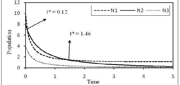
Figure 2: Variation of population against time for a1 = 0.86, a11 = 0.8, a13 = 1.26, d2 = 0.34, a22 = 0.26, a23 = 0.01,

(6)

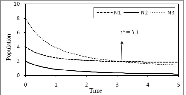
Figure 3: Variation of population against time for a1 = 0.72, a11 = 0.4, a13 = 0.66, d2 = 0.2, a22 = 0.52, a23 = 1.66, d3

= 0.46, a33 = 0.8, N1 = 4, N2 = 2, N3 = 8.

Figure 4: Variation of population against time for a1 = 4.56, a11 = 1.72, a13 = 1.86, d2 = 2.78, a22 = 1.52, a23 = 3.64, d3

= 0.72, a33 = 1.12, N1 = 5, N2 = 3, N3 = 6.

VIII. OBSERVATIONS OF THE ABOVE GRAPHS

Case 1: In this case the self inhibition coefficient of the second species and the natural death rate of the third species are identical. Initially the secondand third speciesdominates overthe firsttill the time instant t* = 0.17 and t* = 0.38 and thereafter the dominance is reversed. Further the initial values of S1, S2, S3 are in increasing order as shown in Figure 1.

Case 2: In this case the natural death rate of S2 is less than of S3. The initial values of S1, S2, S3 are in decreasing order.

Initially the first species is dominant over the second species for a short span and from the instant t* = 0.12 to t* = 1.46 the first species is dominant. This is illustrated in Figure 2.

Case 3: In this case the self inhibition coefficient of S3 is twice of the self inhibition coefficient of S1. Initially the third

species dominates over the first species till the time instant t* = 3.1 and thereafter the dominance is reversed. Further it is evident that all the three species asymptotically converge to the equilibrium point as shown in Figure 3.

Case 4: In this case the third species has the least natural death rate. We notice that the third species has a steep rise initially and then suffers a fall. Further the third species dominates over the other two throughout. (Figure 4).

IX. CONCLUSION

The present paper deals with an investigation on the stability of a syn eco-system consisting of two hosts and one commensal with mortality rate for the second and third species. In this paper we established all possible equilibrium states. It is conclude that, in all eight equilibrium states, only the two states E2 and E6 are stable. Further the global

stability is established with the help of suitable Liapunov’s function and the numerical solutions are computed using Runge-Kutta fourth order method.

REFERENCES

[1] Yu. M. Svirezhev and D. O. Logofet, Stability of Biological Community, MIR, Moscow, 1983.

[2] V. Volterra, Leconssen La Theorie Mathematique De La Leitte Pou Lavie, Gauthier-Villars, Paris, 1931. [3] D. J. Rogers and M. P. Hassell, General models for insect parasite and predator searching behavior:

Interference, Journal Anim. Ecol., 1974, 43, 239 - 253.

[4] V. S. Varma, A note on Exact solutions for a special Prey - Predator or competing species system, Bull. Math. Biol., 1977, 39, 619 - 622.

[5] B. G. Veilleux, An analysis of the predatory interaction between paramecium & Didinium, Journal Anim. Ecol., 1979, 48, 787 - 803.

(7)

ISSN(E): 2277-128X, ISSN(P): 2277-6451, DOI: 10.23956/ijarcsse/V7I7/0198, pp. 215-221 [7] J. M. Smith, Models in Ecology, Cambridge University Press, Cambridge, 1974.

[8] J. N. Kapur, Mathematical Modeling in Biology & Medicine, Affiliated East West,1985.

[9] J. M. Kushing, Integro-Differential Equations and Delay Models in Population Dynamics, Lecture Notes in Bio-Mathematics, Springer Verlag, 1977,20.

[10] W. J. Meyer, Concepts of Mathematical Modeling, Mc.Grawhill, 1985. [11] E. C. Pielou, Mathematical Ecology, John Wiley and Sons, New York, 1977.

[12] N. C. Srinivas, Some Mathematical Aspects of Modeling in Bio-medical Sciences, Kakatiya University, Ph.D Thesis, 1991.

[13] K. L. Narayan and N. Ch. Pattabhiramacharyulu, A Prey-Predator Model with Cover for Prey and Alternate Food for the Predator and Time Delay, Int. Journal of Scientific Computing, 2007, 1, 7 - 14.

[14] K. V. L. N. Acharyulu and N. Ch. Pattabhiramacharyulu, An Enemy- Ammensal Species Pair With Limited Resources - A Numerical Study, Int. Journal Open Problems Compt. Math., 2010,3, 339-356.

[15] B. H. Prasad, A Study on a Four Species Syn-Eco-System Consisting of Host-Commensal, Prey-Predator and Co-Operation with Mortality Rates, Int. Journal of Advanced Research in Computer Science and Software Engineering, 2017, 07(6), 474-479.

[16] B. H. Prasad, A Study on Host Mortality Rate of a Three Species Multi Ecology with Unlimited Resources for the First Species. Journal of Asian Scientific Research, 2017, 07(4), 134-144.

[17] B. H. Prasad, Stability Analysis of a Three Species Syn-Eco-System with Mortality Rates for the First and Third Species. Int. Journal of Physics and Mathematical Sciences, 2016, 06(4), 27-35.

[18] B. H. Prasad, K. S. Rani and P. S. R. Chandra Rao, A Study on Discrete Model of Three Species Syn-Eco-System with Unlimited Resources for the First species. International Journal of Mathematical Sciences. Technology and Humanities, 2016, 6(1), 01-21.

[19] B. H. Prasad, A Study on D iscrete Model of a Prey-Predator Eco-System with Limited and Unlimited Resources. The Journal of Indian Mathematical Society, 2015, 82(3-4), 169-179.

[21] B. H. Prasad, A Study on the Discrete Model of Three Species Syn-Eco-System with Unlimited Resources. Journal of Applied Mathematics and Computational Mechanics, 2015, 14(2), 85-93.

[22] B. H. Prasad, A Study on D iscrete Model of Three Species Syn-Eco-System with Limited Resources. Int. Journal Modern Education and Computer Science, 2014, 11, 38-44.

[23] B. H. Prasad, A Discrete Model of a Typical Three Species Syn- Eco – System with Unlimited Resources for the First and Third Species. Asian Academic Research Journal of Multidisciplinary, 2014, 1, 36-46.

[24] B. H. Prasad, A Discrete Model of Three Species Syn-Eco-System with Unlimited Resources for the Second and Third Species. ZENITH International Journal of Multidisciplinary Research, 2013, 3(12), 42-51.