ISSN: 2278-3369 International Journal of Advances in Management and Economics
Available online at: www.managementjournal.info
RESEARCH ARTICLE
Economic Growth and Foreign Direct Investment: Empirical
Evidence from India during Post-Economic Reforms Era
Singh Surat
1, Singh Dalbir
2*
1 University School of Business, Chandigarh University Mohali, Punjab, India
2Department of Economics, MLN College Yamuna Nagar, Haryana, India.
*Corresponding Author: Email: [email protected]
Abstract
The present study empirically investigates the causality between foreign direct investment (FDI) and economic growth in India over the period 1992-2014, the post economic reforms era. Gross Domestic Product (GDP) has been taken as proxy of economic growth in our study. The study takes into consideration the recent advances in econometric techniques. The study shows the high degree of correlation between GDP and FDI. The variables are tested for stationarity, applying Augmented Dickey-Fuller (ADF) test. The Co-integration test indicates that GDP and FDI are co-integrated time series showing long run equilibrium between the two variables under consideration in India during the study period. To determine the cause and effect relationship between economic growth (GDP) and FDI, Granger Causality test and Vector auto regression (VAR) model have been used. The results suggest that there is bidirectional causality between GDP and FDI. To check the long-run stability the Vector Error Correction Model (VECM) has also been used and the value of the error correction term (ECT) confirms the expected convergence process in the long-run for FDI and economic growth (GDP). The Variance Decomposition also authenticates the cause and effect relationship between GDP and FDI in India.
Keywords:FDI, GDP, India, Correlation, Stationarity, Co-integration, Causality, VECM.
Introduction
In the dynamic age of liberalization, privatization and globalization, foreign direct investment (FDI) which consists of flow of capital, expertise and technology into the host country, has significantly increased in the developing world during the past few decades.
It is considerably true that FDI is one of the most effective ways by which developing economies are associated with rest of the world, as it provides not only capital but also technology and management know-how to the host countries [1]. FDI usually fills up various types of developmental goals as; it reduces saving investment gap by contributing the much needed capital for domestic investment, it reduces foreign exchange gap by generating foreign currency and it reduces tax-revenue gap by accumulating tax revenues [2].FDI may
affect economic growth directly as well as indirectly. Directly, it contributes to capital accumulation and the transfer of advanced technologies to the recipient country whereas indirectly, it enhances economic growth in the recipient country through manpower training, new management practices and organizational arrangements [3].
As far as Indian economy is concerned, after the announcement of liberalized foreign investment policy in 1991, there has been a considerable increase in the FDI inflows. The government of India allowed 100 percent foreign equity participation in high technology and high priority areas like power, drugs and pharmaceuticals, airports, internet service providers, etc. To increase the share of FDI inflows, India eased restrictions on foreign direct investment, strengthened macro-economic stability, instituted domestic financial reforms, capital account liberalization, granted tax incentives and subsidies to attract foreign investors and made the environment conducive for their operations. The inflow of foreign direct investment has increased from US $ 97 million in 1990-91 to US $ 41223 million in 2014-15 (RBI Bulletin). According to the UNCTAD's World Investment Report 2014, India was rated as the fourth most attractive destination for FDI inflows after China, US and Indonesia.
The rising inflows of FDI to India in the post economic reforms era raise the question of how these inflows affect Indian economy and what is the interaction between FDI and economic growth. Therefore this paper has been proposed to explore quantitatively the nature of relationship between FDI and economic growth for India in the post economic reforms era.
Objectives of the Study
This study addresses the following issues:
To analyze the causality between GDP and FDI.
To analyze the stability of equilibrium between GDP and FDI in the long-run.
To examine the Variance Decomposition.Review of Literature
There is a large literature available to address the issue related to the causal relationship between FDI and economic growth [4] examined the relationship between FDI and economic growth for 46 developing countries over the period 1970-1985 and found that the countries which adopted export promotion policy experienced huge economic growth from FDI as compared to those which opted for import substitution strategy. Bende and [5] found in
their study on the impact of FDI through spillover effects on economic growth of ASEAN-5 for the period 1970-1996 that FDI accelerated economic growth either directly or through spillover effects and reported significantly positive impact of FDI on economic growth for Indonesia, Malaysia, and Philippines, while a negative relationship for Singapore and Thailand.
Zhang [6] analyzed the causality between FDI and economic growth for 11 countries in East Asia and Latin America and found five countries, in which economic growth was enhanced by FDI. Campos and Kinoshita [7] analyzed the effects of FDI on economic growth for twenty five Central and Eastern European and former Soviet Union economies and found that FDI had a considerable effect on the economic growth of each selected economy. Liu [8] examined the presence of long run relationship among FDI, economic growth and exports in China during 1981-1997. They found that there is a bi-directional causality among them. A study conducted by Wang [9] on the relationship between FDI and GDP in the sample of twelve Asian economies over the period 1987-1997 suggested that FDI in the manufacturing sector has a significant positive impact on economic growth.
Chowdhury and Mavrotas [10] suggested in their study for causal relationship between FDI and economic growth over the period 1969 to 2000 for Chile, Malaysia and Thailand that GDP caused FDI in the case of Chile and not vice versa, but Malaysia and Thailand both demonstrated a bi-directional Granger causality between the two variables. Hsiao and Shen [11] found a feedback association between FDI and economic growth in China.
through its interaction with the technology gap. A study conducted by Frimpong and Abayie [14] on the causal relationship between FDI and GDP growth for Ghana over the period 1970 to 2005 depicted no causality between FDI and economic growth for the whole sample period and the pre-SAP period. However, FDI caused GDP growth during the post–SAP period. Srinivasanet al. [15] examined the long-run relationship between FDI and GDP for the sample of SAARC nations for the period 1970-2007 and showed a long-run bi-directional causal relationship between GDP and FDI for the sample of SAARC nations excluding India for which they stated unidirectional causal relationship from GDP to FDI.
The present study is an endeavor to investigate the causality and long run relationship between gross domestic product (economic growth) and foreign direct investment in India during the period 1992-2014, the post-economic reforms era, using co-integration test, Granger causality test, VECM and Variance Decomposition under VAR environment.
Data and Research Methodology
The present study is based on secondary data on gross domestic product (GDP) and foreign direct investment (FDI), which has been compiled from Government of India, Economic Survey 2004-05 and 2014-15, Handbook of statistics on Indian Economy 2011-12 and RBI Bulletin, March 2008, June 2014. The study covers the period from 1992-2014, the post-economic reforms era. The aim of this study is to analyze the causality and long-run relationship between economic growth (GDP) and FDI. The recent advances in econometric techniques like the Granger[16] causality test and Vector Autoregression (VAR) techniques have been used to study the cause and effect relationship between GDP and FDI. The major requirement of Granger Causality test is that the variables under consideration must be stationary. To test the non-stationarity in both the variables the unit root test is used.
To examine whether both the time series GDP and FDI are co-integrated, the Johansen co-integration tests have been applied. If the variables are co-integrated, then the model can be estimated at level even if the variables individually are non-stationary. Co-integration confirms that there is long-run relationship (equilibrium) between the variables. To discover the long-term equilibrium and to examine the stability of long run equilibrium between the variables the Vector Error Correction Model (VECM) has been used [17]. To test the normality of the populations from where the samples have been drawn the Jarque-Bera (JB) test is used and to study the correlation between GDP and FDI, the Karl-Pearson’s Correlation Coefficient is computed [18].
Empirical Results
At the outset of the study some preliminary exercises were performed like normality of both the populations GDP and FDI from where the samples have been drawn was checked, correlation between GDP and FDI has been worked out and responsiveness of output (GDP) in relation to FDI has been examined.
Normality: To check normality of both the populations GDP and FDI Jarque –Bera (JB) test of normality is used. The results of (JB) test are presented in Table 1.
Table 1: Results of normality
Mean Std. Dev. Skewness Kurtosis Jarque-Bera CV
GDP 6.44 0.37 0.06 1.95 1.08 0.06
FDI 4.40 0.76 -0.47 2.28 1.36 0.17
Source: Authors’ Calculation
The Jarque-Bera (JB) test follows chi-square distribution for 2 degrees of freedom. The critical value of χ2 at 1 per cent probability level is 10.6. But the calculated values of JB test are 1.08 and 1.36 for GDP and FDI respectively. Since the calculated values of JB test in both the variables are less than the critical value, therefore, we cannot reject
Correlation Analysis: To analyze the
significance of FDI for GDP (economic growth), Pearson’s correlation coefficient has been computed. The results are summarized in Table 2.
Table 2: Results of correlation
GDP FDI
GDP Pearson Correlation 1 0.90*
Significant (2-tailed) .000
FDI Pearson Correlation 0.90* 1
Significant (2-tailed) .000
*Significant at 1% probability level Source: Authors’ Calculation
Since the correlation coefficient between the two variables is fairly high and significant, therefore, the null hypothesis of no correlation between the variables is rejected at 1 per cent probability and the alternative hypothesis of significant correlation between the variables GDP and FDI is accepted. Therefore, the results clearly indicate that there is a significant relationship between
GDP and FDI in India during the study period.
Output Elasticity: Output (GDP) elasticity in relation to FDI has also been examined to know the sensitiveness of output due to the changes in FDI. The double logarithmic analysis has been used. The non-linear function is:
1
. .
u
b t
A FDI e
GDPt t ……… (1)
i. e.,
Log (GDPt) = b0 + b1 Log (FDIt) + ut ……….. (2) Where b0 =Log A
And the elasticity of output is given by:
t
t dLog(GDP )
dLog(FDI )
...(3)
The estimated form of the above equation is:
Log (GDPt) = 4.45 +0.45 FDIt ………(4) S.E = (0.16) (0.04)
t = 27.81 11.25
R2 = 0.89 DW= 1.57
F = 162.43
And
t
t dLog(GDP )
0.45 dLog(FDI )
……….. (5)
This indicates that GDP responds moderately in relation to the changes in FDI. R2= 0.89 being fairly high approves the goodness of fit. The high value of standard F-test indicates that R2 is also significant.
Further in order to analyze the cause and effect relationship and long-run equilibrium between the variables GDP and FDI Granger causality test, Vector
Auto regression (VAR) model and Vector Error Correction Model (VECM) are used. However, before examining the causal relationship between the variables, the first
step is to examine the stationarity of both the time series. The unit root test is used for the purpose.
test at level, first difference and second difference can be written as follows:
1 1
k
t t i t i t
i
Y t Y Y u
……….. (6)1 1
k
t t i t i t
i
Y t Y Y u
………. ....………… (7)1 1
k
t t i t i t
i
Y t Y Y u
………. (8)If =0, then the series is said to have a unit root and is non-stationery. Therefore, if the hypothesis, =0 is rejected for the above equations it can be concluded that the time series does not have a unit root and is
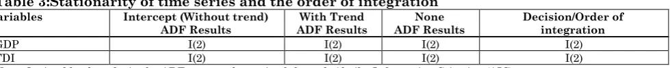
integrated of order zero I(0), i.e. it has stationery properties. The results of ADF test of the concerned series are summarized in Table 3.
Table 3:Stationarity of time series and the order of integration Variables Intercept (Without trend)
ADF Results
With Trend ADF Results
None ADF Results
Decision/Order of integration
GDP I(2) I(2) I(2) I(2)
FDI I(2) I(2) I(2) I(2)
Note: Optimal lag lengths in the ADF test are determined through Akaike Information Criterion (AIC).
Table 3 reveals that both the variables are integrated of order two I(2). In other words, the variables are stationary at second difference. It is quite possible that the two time series share the same common trend (I(1), I(2)….) so that the regression of one on the other will not be necessarily spurious, meaning thereby their linear combination will be integrated of order zero i.e. I(0) and the series will be co-integrated.
Co-integration test: In our study GDP and FDI are found to be integrated of order two i.e. I(2). Under such circumstances, in order to find the long-run relationship between these variables, it becomes imperative to test if these variables are co-integrated. Using the Johansen method of co-integration we test whether the specified variables are co-integrated. The results of the test are being presented in Table 4.
Table 4: Results of johansen Co-integration tests Trend Assumption Co-integration Rank trace
H0 H1 trace
Co-integration Rank max H0 H1 max
Decision/co-integrated Equations
Linear deterministic trend
(unrestricted)
r=0 r>0 27.70*
(15.49)
r1 r>1 4.43*
(3.84)
r=0 r=1 23.27* (14.26)
r=1 r=2 4.43* (3.84)
r = 2
Note: r denotes the number of co-integration(s) exists between the variables. *Significant at 5 per cent probability.
The results of Table 4 reveal that the null hypotheses H0: r=0, H0: r1 against the alternative hypotheses H1: r>0 and H1: r>1 are rejected, because trace statistic exceeds the critical value (in Parenthesis) at 5 per cent probability level implying thereby the null hypothesis of the absence of integration (r=0) and at the most one co-integrating equation (r1) have been rejected at 5% level.
Similarly, H0: r=0, H0: r=1 against the alternative hypotheses H1: r=1 and H1: r=2 are also rejected, because max statistic exceeds the critical value at 5% level. This implies that the null hypothesis of the
absence of co-integration (r=0) and the existence of one co-integrating relation (r=1) appear to be rejected and the existence of two co-integrating relations is accepted at 5% probability level.
inappropriate in the present study because, the variables are found to be co-integrated. However, to authenticate the strong causality between GDP (economic growth) and FDI in India during the study period we discussed the findings of VAR model also.
Therefore, the Granger causality test and VAR model have been used to examine the cause and effect relationship between the variables while Vector Error Correction
Model (VECM) has been used to discover the long-run relationship between the economic variables.
Granger Causality Test: Granger
causality test helps to determine the direction of casualty between the variables under consideration say GDP and FDI in the present model. The test estimates the following pair of regression equations:
1 1 1
1 1
k k
t i t j t t
i j
GDP a FDI b GDP u
……… … (9)1 1 2
1 1
k k
t i t j t t
i j
FDI c FDI d GDP u
……… … (10)Where u1t and u2t are the white noise random disturbance terms and are assumed to be uncorrelated. ‘k' is the maximum number of lags. The optimal lag lengths
have been determined through Akaika’s (1969) information criterion. To test the null hypothesis the following form of standard F-test is used:
1 2 / / k n RSS k RSS RSS F UR UR
R ……… (11)
Where k is the maximum number of lags, n is total number of observations, RSSR is the restricted residual sum of square and RSSUR
is the unrestricted residual sum of squares. The results of Granger causality test are
summarized in Table 5.
Table 5: Results of granger causality
Null Hypothesis F-Statistic P-value
FDI does not Granger Cause GDP 5.10* 0.0193
GDP does not Granger Cause FDI 3.81* 0.0445
*Significant at 5% probability level.
The results indicate that there exists a bi-directional causality between GDP and FDI. The causality runs from FDI to GDP and from GDP to FDI. More precisely, the past-values of FDI significantly contribute to the prediction of present value of GDP even in the presence of past values of GDP. Similarly, the past values of GDP significantly contribute to the prediction of
present value of FDI even in the presence of past values of FDI.
Vector Autoregression (VAR) Model: VAR is another and a better technique to determine the cause and effect relationship between the variables. The test estimates the following pair of regression equations by using OLS method.
k j t k j j t j j t jt a GDP b FDI u
GDP
1
1 1
……….………. (12)
k j t k j j t j j t j
t cGDP d FDI u
FDI
1
2 1
……….……. (13)
The u’s are white noise random disturbance
terms, called impulses, innovations or shocks in the language of VAR. The results of VAR model are presented in Table 6.
Table 6: Vector autoregression estimates
GDP(-1) GDP(-2) FDI(-1) FDI(-2) C R2 F-Statistics GDP SE t-statistic 1.36* (0.19) 6.93 0.33 (0.22) -1.48 -0.45 (0.89) -0.51 3.08* (0.99) 3.11 79196.1 (50930.3)
1.55 0.99 4057.5
FDI SE t-statistic 0.13* (0.05) 2.60 -0.14** (0.06) -2.44 0.51** (0.23) 2.22 0.05 (0.26) 0.20 1464.1 (13318.4)
0.11 0.89 32.86
VAR estimates given in Table 6 reveal that individually, in GDP regression, GDP at lag1 and FDI at lag 2 are statistically significant. This implies that FDI in the presence of lagged values of GDP causes GDP. Similarly, in the FDI regression individually, GDP at lag1 and lag 2 and FDI at lag1 are statistically significant, implying thereby GDP in the presence of lagged values of FDI Causes FDI. Of course, with several lags of the same variables, each estimated coefficient will not be statistically significant possibly because of the presence of multicollinearity in the model. On the basis of standard F-test the null hypothesis that collectively the coefficients may be statistically significant cannot be rejected. In our study the F-value is fairly high, therefore, we cannot reject the hypothesis that collectively all the lagged terms are statistically significant. This implies there is
a strong cause and effect relationship between the variables in the present study.
Vector Error Correction Model (VECM): Co-integration analysis confirms the existence of long-run equilibrium between GDP and FDI in India during the study period. However, it becomes imperative to analyze GDP dynamics following variation in FDI. The variables GDP and FDI are I(2) and co-integrated at level, therefore, the estimation of Vector Error Correction Model (VECM) is pertinent. Further, the stability of the long run equilibrium (relationship) due to the short-run shocks transmitted through FDIt or GDPt can also be studied with the VECM estimation. The model also indicates the speed of adjustment towards the long-run equilibrium after a short-run shock. The model estimates the following regression equations:
1 1 1 3 1 1 1
1 1
n n
t i t i j t i t t
i i
GDP
FDI
GDP
u
………..… (14)2 2 2 4 2 1 2
1 1
m m
t i t j i t j t t
j j
FDI
GDP
FDI
u
………(15)Where GDPt and FDIt are the first differenced series of GDPt and FDIt respectively, u1t-1 and u2t-1 are error correction terms,
1t and
2t are the whitenoise terms. The above equations have been estimated including 2 lags. The results are summarized in Table 7.
Table 7:Results of the VECM estimation GDP
(-1) GDP (-2) FDI (-1) FDI (-2) U1t-1 U2t-1 C R
2 F-
statistic GDP
SE t-statistic
0.36 (0.26) 1.42
0.47*** (0.26) -1.83
-3.26* (1.03) -3.5
-0.44 (1.28) -0.3
0.07* (0.02) 3.35
584575 (166236)
3.52 0.95 56
FDI SE t-statistic
0.42*** (0.22) 1.93
0.93* (0.27) 3.46
0.27* (0.05) 5.05
-0.01 (0.05) -0.19
-0.02* (0.004) -3.84
-126232 (34850)
-3.62 0.67 5.69
*Significant at 1%. **Significant at 5%. ***Significant at 10% probability level.
The findings from the estimated equations (14) and (15) as presented in Table 7 can be interpreted as follows:
The coefficient of error correction term
(ECT) in equation (14) is significant and its sign is positive. This implies GDP is below its equilibrium value, leading GDP to rise in the current year and the speed of rise of GDP in the current year is 7 per cent. In other words, the model suggests that 7 percent of disequilibrium in the previous year is corrected in the current year.
Similarly, the coefficient of error correction
term (ECT) in equation (15) is also significant but possessing negative sign. This implies, FDI is above its equilibrium value, it will start falling in the next period to correct the equilibrium.
Thus the absolute value of 3 and 4 in equation (14) and (15) respectively decides how quickly the equilibrium is restored.
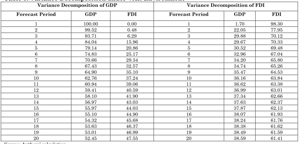
Consequently, the model considers two types of shocks; some shocks are transmitted through FDI channel while others are transmitted through GDP channel. To examine the responses of FDI and GDP to such shocks in the present study the Variance Decomposition under VAR environment is worked out. The Variance Decomposition reflects the proportion of forecast error variance of a variable which is
explained by an unanticipated change in itself as opposed to that proposition attributable to the change in other variables. Variance Decomposition helps to describe the dynamic behaviors of the whole system with respect to shocks. The Variance Decomposition of GDP and FDI variances over 20 years are being presented through the Table 8 given below.
Table 8: Variance Decomposition under VAR Environment
Variance Decomposition of GDP Variance Decomposition of FDI Forecast Period GDP FDI Forecast Period GDP FDI
1 100.00 0.00 1 1.70 98.30
2 99.52 0.48 2 22.05 77.95
3 93.71 6.29 3 29.88 70.12
4 84.04 15.96 4 29.67 70.33
5 79.14 20.86 5 30.52 69.48
6 74.83 25.17 6 32.96 67.04
7 70.66 29.34 7 34.20 65.80
8 67.43 32.57 8 34.74 65.26
9 64.90 35.10 9 35.47 64.53
10 62.76 37.24 10 36.16 63.84
11 60.94 39.06 11 36.62 63.38
12 59.41 40.59 12 36.99 63.01
13 58.10 41.90 13 37.34 62.66
14 56.97 43.03 14 37.63 62.37
15 55.97 44.03 15 37.87 62.13
16 55.10 44.90 16 38.07 61.93
17 54.32 45.68 17 38.24 61.76
18 53.63 46.37 18 38.38 61.62
19 53.01 46.99 19 38.49 61.59
20 52.45 47.55 20 38.59 61.41
Source: Authors’ calculation
The Variance Decomposition of GDP reveals that in the short-run, for example in the third year, impulse or innovation or shock to GDP account for 93.71 percent variation of the fluctuation in GDP (own shock). On the other hand, the shocks transmitted through the channel FDI can cause 6.29 percent fluctuation in GDP.In the long-run, for example in 20th forecast period, the shock to GDP can contribute 52.45 percent variation of the fluctuation in GDP (own shock), while an impulse in FDI can cause 47.55 percent fluctuation in GDP. This implies that the contribution of shock to GDP in the
fluctuation of GDP itself is decreasing in the long-run while that of FDI is increasing. Similarly, the Variance Decomposition of FDI indicates that in the short run say in
the third year, shock to FDI causes 70.12 percent of the fluctuation in FDI (own shock), while the impulse in GDP contributes 29.88 percent of the fluctuation in FDI. In the long-run, that is, in 20th forecast period, the shock to FDI account for 61.41 percent variation of the fluctuation in FDI itself (own shock), while an innovation (impulse) in GDP causes 38.59 percent fluctuation in FDI. This indicates that the contribution of shocks to FDI in the fluctuation of FDI itself decreases in the long-run, however, the contribution of the shocks to GDP in the fluctuation of FDI increases. This further authenticates the feedback (bidirectional) causality between economic growth (GDP) and FDI.
Policy Implications
The findings of the study have important policy implications as follows:
FDI must be attracted to raise the GDP growth rate substantially.
Political stability and good governance is also must to attract more FDI.
The government must device the policy to educate the people and make them to
realize the importance of FDI for the welfare of the nation in general and individuals in particular.
Conclusion
The results of our analysis reveal that boththe populations (GDP) and FDI are normal and significantly correlated with each other. The elasticity of output (GDP) in relation to the changes in FDI is found to be 0.45.The study has found evidence that FDI has a significant role in explaining variations in economic growth (GDP) and vice-versa in India over the study period. It is observed that FDI Granger caused GDP and GDP Granger caused FDI. That is, there is
bidirectional relationship between economic growth (GDP) and FDI during post-economic reforms era. The Vector Error Correction Model (VECM) has explained the dynamic adjustment process and long-run relationship between GDP and FDI over the study period. The Variance Decomposition in VAR environment also testifies that there is bidirectional relationship between GDP and FDI.
References
1. Pradhan, R P (2006) FDI in the Globalization Era: Chinese and Indian Economic Growth, Prajnan, 34: 323-343.
2. Vadlamannati KC, Tamazian A, Irala LR (2009) Determinants of Foreign Direct Investment and Volatility in South East Asian Economies, Journal of the Asia Pacific Economy, 14: 246-261.
3. De Mello, LR (1999) Foreign Direct Investment Led Growth: Evidence from Time Series and Panel Data, Oxford Economic Papers, 51 (1): 133-151.
4. Balasubramanyam VN, Salisu M, Dapsoford D (1996) Foreign Direct Investment and Growth in EP and IS Countries, Economic Journal, 106: 92-105.
5. Bende-Nabebde, A (2001) FDI, Regional Economic Integration and Endogenous Growth, Some evidence from Southeast Asia, Pacific Economic Review, 6(3): 383-399. 6. Zhang K H (2001) Does Foreign Direct
Investment Promote Economic Growth? Evidence from East Asia and Latin America, Contemporary Economic Policy, 19(2):175-1. 7. Campos N F, Kinoshita Y (2002) Foreign
Direct Investment as Technology Transferred: Some Panel Evidence from the Transition Economies, CEPR Discussion Paper 3417. London: Centre for Economic Policy Research. 8. Liu X, Burridge P, Sinclair P J N (2002) Relationships between Economic Growth, Foreign Direct Investment and Trade: Evidence from China, Applied Economics, 34: 1433-1440.
9. Wang M (2002) Manufacturing FDI and Economic Growth: Evidence from Asian Economies, Mimeo: University of Oregon Mimeo.
10. Chowdhury A, Mavrotas G (2003) FDI and Growth: What causes what? World Institute for Development Economics Research (WIDER) Conference on Sharing Global Prosperity.
11. Hsiao C, Shen Y (2003) FDI and Economic Growth: The Importance of Institutions and Urbanisation, Economic Development and Cultural Change, 51(4): 883-896.
12. Marwah K, Tavakoli A (2004) The Effects of Foreign Capital and Imports on Economic Growth, Journal of Asian Economics, 15: 399-413.
13. Li X, Liu X (2003) Foreign Direct Investment and Economic Growth: An Increasingly Endogenous Relationship, World Development, 33(3): 393-407.
14. Frimpong J M, Abayie E F O (2006) Bivariate Causality Analysis between FDI Inflows and Economic Growth in Ghana, International Research Journal of Finance and Economics, Issue 15.
16. Granger C W J (1969) Investigating Causal Relations by Econometric Models and Cross-spectral Methods, Econometrica, 35: 424–438. 17. Engle, R.F. and Granger, C.W.J. (1987),
Cointegration and Error Correction Representation, Estimation and Testing, Econometrica, 55: 251-276.
18. Gujarati D N (1995) Basic Econometrics, 4th Edition, New York: McGraw-Hill.