Thesis

(1)

The Mathematics of Sinking

Through Sharply Stratified

Liquids

An Experimental Approach with Spheres

Jacob Dylan Bruney

An Honors Thesis Presented for the Department of Mathematics at UNC Chapel Hill

Mathematics UNC Chapel Hill

United States 10/9/2015

Approved:

(2)

The Mathematics of Sinking Through

Sharply Stratified Liquids

An Experimental Approach

Jacob Dylan Bruney

Abstract

(3)

Acknowledgments

None of this project would have been possible if not for my amazing adviser, Roberto Camassa. I must have approached him only a few days before the dead-line for submitting a thesis proposal. I had no adviser and no idea of what I was interested in studying. By some spark of insanity, Professor Camassa agreed to help me out, a true testament to his character and interest in the academic am-bitions of his students. As busy of a man as Professor Camassa is, it amazes me how he somehow found the time to meet with me, direct my studies and keep a good tally of my progress (an impressive feat for a man who juggles a small army of graduates). I owe this project to his intelligent and caring guidance. Thank you for everything professor!

In the summer before I started this thesis, I vividly remember a conversation I had with a graduate student. I asked her about the thesis. What is the honors thesis? Is it worth my time? And am I even capable enough to finish it? To which she responded, to the best of my memory, ”Dylan, you should definitely do it! And if it doesn’t work out, which can’t even happen, you will still learn a lot from it. And don’t worry, I’ll be there if you need any help.” That graduate student was Claudia Falcon and that advice gave me the confidence I needed to start this long endeavor and difficult undertaking. Every step of the way, she was always there to offer a helping hand. This testimony doesn’t do her any justice, especially in consideration of the many long hours she would spend with me weekly. Thank you Claudia for everything! If you are ever in need, I will be there as a colleague and a close friend.

I also must mention Professor Richard McLauglin and Professor Daniel Harris. Having no real obligation to help me, they found the time in there busy schedules. You guys are awesome!

Lastly, I should thank Claudia’s little helpers Sabina Iftikhar and Gabriella Stein. Although I can’t overemphasize how many times they helped me in my experiments, their largest contribution, by far, was their great personalities and friendship. They made the lab a fun place to work, and helped me get through the grind of running these long experiments.

(4)

1

2 Introduction

Density stratification is a key process on Earth. It manifests in many natural forms, from governing pollutants in the atmosphere, to oil leaks in the ocean. However, one of the most important and delicate mechanisms that it governs is the carbon cycle of the ocean. As global temperatures rise, the process by which the ocean recycles carbon gas into the atmosphere is changing in currently unpredictable and detrimental ways. In this paper, we will better understand this phenomenon by studying the mathematics that govern the descending of glass spheres in a stratified regime, a substitute for marine ag-gregates/ marine snow in the ocean (a crucial part of the carbon cycle). Of particular interest is the low-Reynolds two-spheres, two-layers regime. This thesis will follow the path of my research. Beginning with a literature review as a basis for my work, the paper will progress from rudimentary mathemat-ical observation, to experiments. The progression of experiments will be in this order: two spheres in water, two spheres in homogenous corn syrup, and lastly two spheres in stratified corn syrup. The paper will be brought full circle with mathematical conclusions from the analyzed observations.

3 Literature Review

Up to this point, there have been great strides in empirically pre-dicting a rigid sphere falling in a homogeneous regime. However, due to the currently unsolved 3-dimensional Navier-Stokes equa-tions, the coefficient of drag has only been empirically derived or approximated with solvable simplifications of Stokes Flow (which is a simplification itself ). These text explore that derivation:

(Clift, R.,Grace, J.R., and Weber, M.E., 1978)- ”Bubbles,Drops, and Particles” is a comprehensive study on predicting rigid objects in low Reynolds regimes. The research, compiled by three chemical engineers, dis-cusses the numerous drag coefficients that had been derived over the years, and offers a new empirically derived equation for the coefficient.

(7)

that could approximate the drag coefficient ”over the entire Reynolds-number range of the available experimental data”, and is developed, then analyzed in this paper.

For predicting the velocities of two spheres in homogeneous low Reynolds solutions there are a number of early papers that provide analytic approximations which they compare to their experimental data:

(Kynch, G. J. 1958) Kynch derives and approximate model for the velocity of two spheres in low Reynolds as a function of separation and radii. He corroborates his model with his own experiments, and finds the match ”favorable”. Most importantly, he states ”Equal spheres falling under gravity fall together with a constant separation, but they only fall vertically when the line of centres is either horizontal or vertical; otherwise they tend to slide downwards along the line of the centres.”

(Davies, G. A. and, Rushton, E., 1973) They try to build upon earlier work, like Kynch’s, by simplifying the situation further and limiting their configurations for the two spheres, specifically to the co-axial (snow-man/stacked) case. They develop a general solution for creeping flow, and believe it agrees with solutions previously published.

For sharply stratified regimes, a lot of the research comes from UNC’s Fluids Lab department:

(Abaid, N., Adalsteinsson, D., Agyapong, A. and McLaughlin, R. M.,2004)

One of the first analysis into the ”floating” effect of a falling sphere due to the entrainment around a sinking sphere of lower density top layer fluids, in a more dense, bottom layer fluid. This paper acts as a starting point for my research into the properties and equations that govern a sphere descending in a sharply stratified low Reynolds regime.

(Roberto, C., Falcon, C., Lin, J., McLaughlin, R., Mykins, N., 2009)

(8)

regime. With the help of a Green’s function formulation, they develop a numerical model of the forces caused by the entrainment of a sphere, and then compare there computational method to experiments ran in the lab. Of particular interest is their investigation into the velocity fields created by the entrainment.

This Paper

This paper is a progression and, ultimately, a union of the aforementioned papers. Attempting to wed the models of two sphere configurations with the effect of entrainment. This paper also reports the first recorded observance of the approach of two spheres in the bottom layer of a sharply stratified due to the force of entrainment.

4 Terminal Velocity of a Single Sphere in Low

Reynolds Free Space

A single sphere’s fall is governed by three forces, Gravity, Buoyancy and Drag:

(Gravity and Buoyancy) 4 3πr

3₍_ρ

particle−ρf luid)g

(Drag) 1 2πr

2_C

dρf luidV2

Likewise Newton’s second law:

(Total Force =M ass·Acceleration) −4

3πr

3_ρ

particle

dV dt

These forces are collectively represented in the equation:

4 3πr 3_ρ particle dV dt = 4 3πr

3₍_ρ

particle−ρf luid)g+sign(V)

1 2πr

2_C

dρf luidV2

(9)

WhereV =Velocity,t=Time,µ=Dynamic Viscosity,r=Radius,ρ=Density, and g =Gravitational Constant.

We can solve for the terminal velocity at low Reynolds (Reynolds 1) by first replacing our coefficient of friction (Cd) with the Reynolds dependent

function for stoke flow 24/Re. Then since terminal Velocity is a constant,

dV

dt = 0, which makes the left hand side of (equation 1) zero. Lastly, by

moving and collecting terms we get:

Vterminal =

2r2₍_ρ

f luid−ρparticle)g

9µ

(Equation 2)

5 Elementary models to predict two spheres

falling:

Suppose we drop two identical spheres lined horizontally and tangential (symmetry and low Reynolds reversibility should guarantee there velocities are identical), whereVt1 is the terminal velocity of one of our spheres andVt2

is the terminal velocity of both our spheres with the respective assumption: (1)What if we just treat this as a sphere with twice the radius?

Vt1 =

2r2(ρf luid−ρparticle)g

9µ Vt2 =

2(2r)2₍_ρ

9µ

= 8r

2₍_ρ

9µ //

= 4(2r

2₍_ρ

9µ )

⇒4Vt1 =Vt2

(10)

”Volume of a single sphere”=v1=

4 3πr

3

1 ⇒r1 =

3v1

4π 1/3

”Volume of hypothetical sphere”=v2=2v1=4 3πr

3 2

⇒r2 =

3(2v1)

4π 1/3

= 21/3₍3v1

4π 1/3

)

⇒21/3r1 =r2 (Substitution)

⇒22/3_V

t1 =Vt2 (Same steps as in (1))

(3) What if we just treat this as a sphere with twice the ra-dius and compensate for the density by calculating the density of a sphere with twice the radius that inscribes the two particles and fill the rest with the surrounding fluid?

Lets first concentrate on how changing the density calculation effects our terminal velocity.

Vt1 =

2r2₍_ρ

f luid−ρparticle1)g

9µ

For the term (ρf luid−ρparticle1) of our second particle:

ρparticle2 =ρparticle1

VtwoP articles

Vtotal

+ρf luid

Vf luid

Vtotal

= ρparticle1

4 +

3ρf luid

4 (Simple volume calculation)

Vt2 =

2(2r)2₍_ρ

f luid−(

ρparticle1

4 +

3ρf luid

4 )g 9µ

= 4(

2r2₍ρf luid−ρparticle1

4 )g

9µ )

= (4·1

4) 2r2₍_ρ

f luid−ρparticle1)g

9µ

⇒Vt1 =Vt2(Substitution)

(11)

Since ρ=mass/volume ⇒ρparticle2 = 2ρparticle1

Thus: Vt2 =

2r2₍_ρ

f luid−2ρparticle)g

9µ

= 2r

2₍_ρ

9µ +

2r2(ρparticle)g

9µ

⇒Vt1+

2r2_g

9µ ρparticle =Vt2

These naive models give us a good understanding of some possible upper bounds, and certainly suggest that two spheres will sink faster then one.

6 Developing a Drag Coefficient for Finite

Reynolds

The crucial, and Reynolds dependent, drag coefficient of our terminal velocity equation has been approximated by various calculations. Although these ap-proximations are nearly identical in Low Reynolds regimes (as they should all converge to Stokes), they tend to diverge from each other at Re > 1. To begin, the simplest and easiest drag coefficient to calculate is just the stokes defined drag coefficient. Since this calculation is straightforward, I will quickly walk us through it:

Fd= 3πµU d(Stokes Definition for Drag Force)

and

Cd =

2Fd

ρU2_A(Definition of Drag Coefficient)

⇒Cd=

µ24

ρU d

Since, Re= ρU d

µ

⇒Cd=

24

(12)

Where, d is our sphere’s diameter, A =πd2/4 is the cross sectional area of our sphere, µ is are dynamic viscosity, ρ is our fluid density, and U is our fluid velocity (relative to sphere)

Stokes drag is accurate only for low-Reynolds flow (at higher Reynolds, stokes equation makes thing impossible to calculate analytically).

In the Early 1900’s, Oseen built upon Stokes calculation by correcting for an originally neglected inertial effect and derived the following approxima-tion:

24[1 + 3Re/16]

Re

Then in 1978 R. Clift, J. Grace, and M. Weber, M.E., did a comprehensive study into all the work that had been produced to approximate the coefficient of drag, across the range of feasible Reynolds values. They even provided a table of the many empirically derived coefficients of drag.

Then presented their own which represented a larger span of empirical data 1< Re <1000:

Cd=

24[1 + 0.15Re0_.₆₈₇ Re

(Clift et al., 1978)

(13)

(14)

(15)

7 Terminal Velocity of a Single Sphere Finite

Reynolds

To continue this investigation, we need to be aware that we are operating on the cusp of what many believe to be low Reynolds versus finite Reynolds. What differentiates the two is the complexity and magnitude of the coeffi-cient of drag. In the low Reynolds case our coefficoeffi-cient of drag was 24/Re, which simplified equation 1 to equation 2, but at this point, it may be more accurate to use different coefficients.

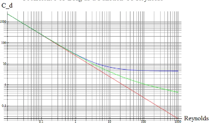
Dr. Faith Morrison from M.I.T. in her paper ”Data Correlation for Drag Coefficient for Sphere” develops a equation for the drag coefficient that uses data correlations from experiments to provide a reasonably accurate data set from low Reynolds flow to high. More specifically, she cites her equations being accurate for low-Reynolds all the way up to Reynolds of 107, cover-ing a large spectrum of the available experimental data. However, as shown in the model graph below, the equation for the drag coefficient is actually piecewise. ForRe < 2 the drag coefficient is 24/Re (creeping Reynolds), the stokes coefficient for low Reynolds. For the range of 1 < Re < 106 (recir-culating) it uses the provided, empirically derived, drag coefficient. Lastly, for 106 < Re < 107 (turbulent) the equation models uniform flow around a sphere with ”a line with slope of 0.80 on a log-log graph”.

To recap, equation 1 for Reynolds: 4 3πr 3_ρ particle dV dt = 4 3πr

3₍_ρ

particle−ρf luid)g−sign(V)

1 2πr

2_C

dρf luidV2

Where Morrison’s coefficient is:

Cd =

24

Re+

2.6(Re 5 ) 1 + (Re

5 )

1.52

+

.411( Re 263000)

−7.94

1 + ( Re 263000)

−8

+ Re

0.8

461000

(16)

Just to make sure, graphing it ourselves:

(17)

Now we can observe how for very large Reynolds values, the slope is almost linear, and less then 1 (drag always reduces velocity). Lets look closer at the left side of that hump:

(18)

So, it appears that the coefficient asymptotically approaches infinity on the y axis, this explains the high numbers for low Reynolds. But what does it approach for certain? Although Morrison advises to use 24/Re for low Reynolds, we should take a moment to see how her experimental coefficient acts around 0.

8 Taylor Approximations:Morrison’s

Coeffi-cient As Reynolds Approaches Zero

Examining How the Equation Acts:

We need to move all parts of this equation that are functions of Reynolds to one side of the equation so that we can observe the behavior as Reynolds approaches zero.

Since we are focusing on terminal velocity, the left hand side of: 4

3πr

3_ρ

particle

dV dt =

4 3πr

3₍_ρ

particle−ρf luid)g−sign(V)

1 2πr

2_C

dρf luidV2

(19)

reorganizing the other two terms, gives us: 8r(ρparticle−ρf luid)g

3ρf luid

=V2Cd

Since velocity can be rewritten as a function of Reynolds:

Re= V rρf luid

µ ⇒V

2 _{= (} Reµ rρf luid

)2 (Substituting into our equation)

⇒ 8r

3_ρ

f luid(ρparticle−ρf luid)g

3µ2 =Re

2_C

d

Now Concentrating on the right side. We get:

Re2_C

d= 24Re+

2.6(Re

3

5 ) 1 + (Re

5 )

1.52

+

.411( Re 263000)

−5.94

1 + ( Re 263000)

−8

+ Re

2.8

461000

To simplify this further lets expand these term by there Taylor series at 0, up to order O[Re]3.

For the first term 24Reit is it’s own Taylor series, so we will leave as is: 24Re

(First Term)

For the second term

2.6(Re

3

5 ) 1 + (Re

5 )

1.52

, we will make a adjustment by assuming

(Re/5)1.52_≈₍_Re/₅₎1.5_{. Now by substituting the powers we get:}

325(Re

3/2

53/2 2

)

1 + (Re

3/2

53/2 )

Taylor expanding this series where x= Re

3/2

53/2 :

(20)

Truncating at O[Re]3 ⇒O[x2] gives us:

325(x2)⇒2.6Re3 (Second Term)

For the third term

.411( Re 263000)

−5.94

1 + ( Re 263000)

−8

, we will make a adjustment by assuming

(Re/263000)−5.94≈(Re/263000)−6. Now substituting the powers we get:

.411∗2630002( Re 263000)

−6

1 + ( Re 263000)

−8

Taylor expanding this series where x= Re 263000:

.411(2630002)(x2−x10 +x18−x26 +...)

Truncating at O[Re]3 _⇒_O_[_x3_{] gives us:}

.411(263000)(x2)⇒.411Re2 (Third Term)

Lastly, for the forth term: Re

2.8

461000, we will make a adjustment by assuming (Re)2.8 _≈ ₍_Re₎3_{. Now we end up with} Re

3

461000, which would combine with our second term. But since the coefficient 1/461000 = 2.169∗10−6 ₂_.₆

(the coefficient of the second term),we will neglect this term. Thus our final Taylor Approximation for Reynolds around 0 is:

⇒ 8r

3_ρ

f luid(ρparticle−ρf luid)g

3µ2 = 24Re+.411Re

2_{+ 2}_.₆_Re3

(equation 4)

(21)

that the particle would remain stationary in the liquid. This means that velocity at this point is also zero. As expected once you consider that

0 = Re = V rρf luid

µ , since the density of the fluid and the radius of the

particle are non zero for any given scenario, the velocity must be zero. This then agrees with our conclusion.

Examining how Cd acts

To observe Cd’s behavior we nullify multiplying through by the Re2

con-tributed by theV2 term by dividing the RHS of equation 4 byRe2, giving us: 24/Re+.411 + 2.6Re=Cd

which approaches infinity as Reynolds approaches zero. This is in agreement with our graph.

9 Boundary Condition

Before we begin our experiments, there remains one essential caveat for pre-dicting the terminal velocity; a boundary condition to account for not being in free space (these experiments will be conducted in cylindrical tanks). This boundary condition has a well known derivation [available in (Camassa et. al.) paper if curious), that uses the Faxen’s law. Faxen’s law, developed much later in this paper, relates the forces of sphere from the flow in the tank. This addition can compensate for the addition of walls using the ”method of reflections”. This compensation for flow using Faxen’s Law is called the ”Faxen correction”. For Newtonian fluids, a sphere falling through a cylin-drical tank will have the following Faxen Correction (where R is radius and

a is the radius of the sphere:

KN(

a

R) = [1−2.10444( a

R)+2.08877 a R 3

−0.94813(a

R) 5₋

1.372(a

R) 6

+3.87(a

R) 8₋

4.19(a

R) 10

(22)

10 Experiment Setup and Analysis:Visual

(23)

Analysis

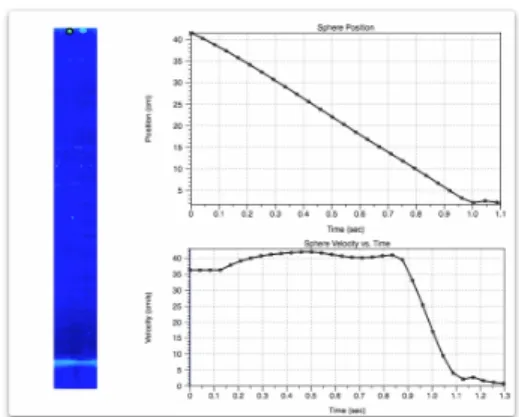
This is just a brief note on how analysis was conducted. To extract data from the videos, I used a program for data processing (especially videos) called DataTank. Developed in large by a UNC professor, and available on Apple iOS, DataTank was used for constructing all velocity profiles that you will see throughout this paper. The method of tracking used depended on the exper-iment, but was predominately through a technique called ”color distance”. Basically, the program takes a single frame of the video and assign a nu-meric value to each pixels color. By specifying a specific color and tolerance, DataTank would be able to differentiate colors within that tolerance from the rest of the frame. After finding those pixels within the tolerance, and as long as ”enough” are in one spot, the program finds the ”center” of these pixels and records its location. As the video evolves, the color moves with the object I am tracking, and thus new locations are recorded at different times. Using this location value and time, it creates a discrete velocity profile from which, using familiar computational methods, creates a continuous velocity profile from which I gather my data.

(24)

(25)

11 Experiment One: Two Identical Spheres

in Homogeneous Water

Date:10/6/2015

Problem and Purpose: To begin my investigation, I started with the simplest case that would still exhibit the behavior we were after, dropping two identical spheres through a homogeneous solution of salt water. This experiment would provide me the opportunity to become familiar with lab protocol, the equipment and material available to me in the lab, and the process of performing experiments of this type. This experiment will also confirm some basic equations and most importantly, it will guide further de-velopment of this paper.

Materials:

-D7000 Camera (Video Mode Recording)

-Large Plastic Cylinder Tank with Diameter of Approximately 19.2 cm -Salt Water of Density 1.1774 g/cm3, Assumed viscosity (mP a.s)_≈1 -Ruler (12 inch)

-Giant Plastic Spoon for Retrieval -Camera Mount

-Sphere Red, Radius(cm)=0.296545, Density(g/cm3)_≈2.26 -Sphere Black, Radius(cm)=0.296545, Density(g/cm3₎

≈2.26

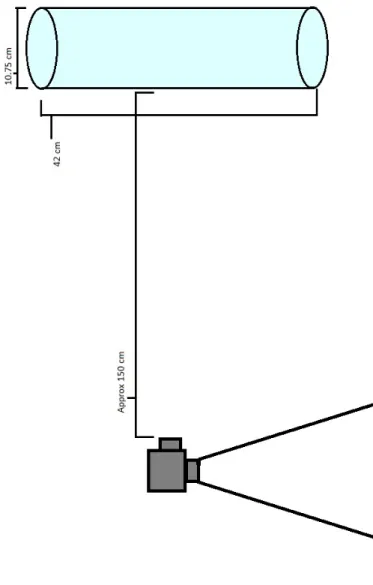
Set-up:The experiment was performed by first filling up the cylindrical tank with the saltwater from the lab’s reservoir tank. The density of the wa-ter was then checked with the portable density mewa-ter. The tank was moved to the table where I then placed a grided backdrop. Using adhesive putty, I stuck a ruler to the side of the tank so that the side with measurement notches would be facing the camera. I then set up the camera on the stand, focused it on the ruler (the plane where the sphere would be dropped) and stabilized at an appropriate height. Lastly, I set up the lighting apparatus on a rig behind the camera.

(26)

drops of a single red then black sphere, so as to have three videos for each situation.

Results:

Type Terminal Velocity* Error

Single Sphere Predicted (Morrison’s Coeff.)) 39.5845 NA

Single Sphere (Red) 41.93188 5.93%

Single Sphere (Black) 39.63765 .134%

Double Sphere (Horizontal)(Red) 40.74412 NA Double Sphere (Horizontal)(Black) 41.33375 NA

* Calculated by average of the maximum velocity from tracking and the two velocity points beside it.

(27)

Figure 7: Double Sphere (Horizon-tal) (Red)

Figure 8: Double Sphere (Horizon-tal)(Black)

Issues: As observed by the lack of data, the lighting needs to be improved as to minimize shadows, so that more positions can be tracked. It should also be mentioned that a sinusoidal falling pattern created a poor data set of the ”true” velocity since DataTank was only tracking the vertical descent (would have been higher). As recommend by Doctor Camassa and Graduate Claudia Falcon, a more viscous fluid will prevent this behavior, creating a less deviated linear path from top to bottom by minimizing/removing the ”vortex rings” that it creates on its descent. Likewise, the more vicious sub-stance will allow for more data points as the sphere takes longer to fall from top to bottom. Also, the camera was not focused enough and adjustments could be made to the aperture and shutter speed.

(28)

12 Experiment Two: Two Identical Spheres

in Homogeneous Corn Syrup

Date:10/12/2015

Problem and Purpose: So now that I had some experience in the lab and some clear evidence of two spheres falling faster then one, I followed the recommendation of my adviser, and transitioned to corn syrup, where the dampening of the sinusoidal behavior, the low Reynolds domain, and presence of more data will allow for a more accurate representation of this effect. Likewise, I will be performing multiple analysis on each configuration, experimenting with different methods of releasing the sphere and trying new configurations. This shall be the precursor to moving to a stratified regime and the actual behavior we are trying to observe.

Materials:

-D7000 Camera (Manual Mode Button Press Interval Shooting)

-Small Plastic Cylinder Tank with Diameter of Approximately 10.75cm -Corn Syrup of Density of Approximately 1.36672 g/cm3 at 22.65 C (Den-sity, Viscosity and Temperature was measured four days after experiment), Viscosity 22.1281 P a.s

-Camera Mount -Plastic Wrap -Metal Mixing Pot

-Giant Plastic Spoon for retrieval and stirring

-Sphere Red, Radius(cm)=0.296545, Density(g/cm3₎

≈2.26

-Sphere Black, Radius(cm)=0.296545, Density(g/cm3₎

≈2.26

(29)

camera on the ruler (the plane that the sphere should fall in).

Procedure: The experiment was performed in the following manner. First I alternately dropped a single black sphere, then a single red. This, pattern was repeated three times, however, only two videos of the black sphere and one of the red where suitable for keeping after later analysis. I then conducted three drops with the ”Snowman” configuration of vertical aligned tangential spheres, only one of which were appropriated for analysis. Lastly, I performed four videos of a vertical alignment, only two of which were suitable for analysis. After each drop, the spheres were removed from the bottom using the giant plastic spoon, partially submerging my hand, then quickly cleaning the apparatus and the sphere. The camera was set to a manual mode, where it would take 1 second photos as long as I held the button. After dropping the spheres I would immediately press the button and wait till they reached the bottom of the tank to release.

Results:

Type Terminal Velocity Average Prediction Error

Single Sphere Predicted 0.740808 NA NA

(30)

Figure 9: Single Sphere (Red)

Figure 10: Single Sphere (Black)

(31)

Figure 12: Double Sphere (Hori-zontal) (Red)

Figure 13: Double Sphere (Hori-zontal) (Black)

Figure 14: Double Sphere (Hori-zontal) (Red)(2)

(32)

Figure 16: Double Sphere (Vertical/Red-on-Black)(Red)

Figure 17: Double Sphere (Vertical/Red-on-Black)(Black)

Issues: The cameras lighting looked good on digital display while record-ing, but during analysis it became apparent it could have been brighter. Shadows from the top of the tank and the reflection of the light prevented good tracking for the first part of the drop. Likewise, the bottom part of the drop remained unanalyzed due to some finicky lighting behavior toward the bottom. The markers coloration on the spheres was slowly eroded as tests where performed, and although I recolored it twice during the exper-iments, it would have been much easier to track with a darker, even coat that didn’t remove itself. When I would retrieve the sphere with the spoon, I would introduce bubbles and get my hand extremely sticky. Also, on a couple occasions after cleaning the spoon in a nearby wash pot, I introduced water into the upper levels of the corn syrup. Although I settled on my fin-gers, the funnel and two pieces of cardboard (acted as a vice) that I used for dropping, caused very horrendous looking drops that ultimately could not be used. Even still, my fingers were very much imperfect and the boundary layer they created caused a uneven drop. Also, since I had to hold the camera button down while shooting, I couldn’t replace the plastic wrap as the video ran, meaning the top part of the corn syrup was evaporating and becoming more dense then it should have. Lastly, there should have been more pictures taken and used. There was simply not enough data points, that covered to little of the range of the corn syrup in the tank, and not enough videos of each method of dropping.

(33)

elimi-nated the sinusoidal falling behavior as predicted, got more data points, and produced precise and consistent plots and data. However, we have a huge discrepancy in our theoretically predicted terminal velocity and our experi-mentally observed. As noted by Claudia Falcon, the camera is inconsistent with interval shooting, so we will be using video mode next time. Likewise, we will be taking viscosity the day of.

13 Error Propagation

Ultimately, the tools that I am using to perform measurements are inaccurate to some mechanical degree, and small deviations from the true measurements can grow exponentially while using the high order and many termed equa-tions that I am using for predicting terminal velocity of a single particle. As of such, it is of utmost importance that we look at how these errors can prop-agate and contribute for each function for our Coefficient of Drag: Stoke’s, Oseen’s, and Morrison’s.

Errors from Each Tool

Scale error = 5∗10−4 _{grams as stated by manufacturer’s website}

Caliper error =.0001 inches from observation

Density meter error =.00001g/cm3 as stated by manufacturer’s website Viscometer error = .5 percent of dynamic viscosity as stated by manufac-turer’s website

How that Showed in Experiment Two

Mass =.247033 (Measured Mass in grams)

Radius =.2975991 (Converted Measured Radius in cm) Fluid Density= 1.36672 (Measured Density ing/cm3₎

(34)

can be achieved with that error in mind. Stoke’s

This is the easiest to start with as the Cd = 24/Re simplifies equation 1

dramatically, to equation 2.

With Measured Values:VT erminal= 0.795702

With Maximum Error:VT erminal = 0.801771

At values:

-Mass = 0.247533 grams

-Radius= 0.2974721 centimeters -Density of fluid= 1.33671 g/cm3

-Dynamic Viscosity of Liquid = 21.13 pascal seconds Oseen’s

At values:

-Dynamic Viscosity of Liquid = 21.13 pascal seconds Morrison’s

At values:

(35)

Conclusion: So it seems that instrument error can’t account for the massive discrepancy. Although this was calculated for a particular experi-ment, this could have readily been generalized. Whats important is that the order of this error will remain constant across the experiments of this paper and thus, negligible compared to the error we are seeing. This leaves two possibility in my mind, either I messed up as an experimenter, or the camera was inaccurately taking interval shots (suggested by mentor Claudia Falcon). Either way, a retest is in order that will attempt to anticipate and eliminate these possibilities.

14 Experiment Three: Re-Test Two

Identi-cal Spheres in Homogeneous Corn Syrup

Date:11/11/2015

Problem and Purpose: In an attempt to find the source of the dis-crepancy between the calculated and the experimental terminal velocity, a re-test was needed. To eliminate some errors: this test will be performed by multiple experimenters and tracked with video shooting to get more frames, all density and samples will be collected the day of the experiment, we will be concentrating on replacing the plastic wrap covering between test to prevent evaporation, and we will attempt to reduce foreign liquids and air bubbles from entering the corn syrup. This test will have a focus on single drop and double vertical drop tests with different distances to provide a stronger tran-sition to a two layered regime.

Materials:

-Small Plastic Cylinder Tank with Diameter of Approximately 10.75cm -Corn Syrup of Density 1.36902g/cm3 _{at 22}_.₉₀_C _{with a Dynamic Viscosity}

of 23.632 Pascal Seconds -Camera Mount

-Plastic Wrap -Metal Mixing Pot

(36)

≈2.26

-Sphere Black, Radius(cm)=0.296545, Density(g/cm3)_≈2.26

Set-up: Corn syrup from Experiment Two was poured into the metal mixing pot and a small amount of additional corn syrup was added from the stored containers. It was then stirred for 40 minutes, poured back into the cylinder, covered in two layers of plastic wrap to prevent evaporation, and left over two nights. The day of the experiment (with the assistance of Gabbi and Claudia Falcon), the density was taken, as well as a sample for the viscometer. The camera was mounted, balanced and focused. Lastly, paper towels were procured from the bathrooms and the sphere were recolored with marker.

(37)

Type Terminal Velocity Predicted Error Single Sphere (Red)(1) 0.795560 0.639114 24.47% Single Sphere (Black)(1) 0.826212 0.639114 29.27% Single Sphere (Red)(2) 0.807280 0.639114 26.31% Single Sphere (Black)(2) 0.808012 0.639114 26.42% Single Sphere (Red)(3) 0.794257 0.639114 24.27% Single Sphere (Black)(3) 0.826110 0.639114 29.26% Double Sphere

(Vertical/Red-on-Black/0.10cm)(Red)(1)

1.208318 0.999232 20.92%

Double Sphere

(Vertical/Red-on-Black/0.10cm)(Black)(1)

1.194725 0.999232 19.56%

Double Sphere

0.875607 0.723706 20.99%

Double Sphere

0.858294 0.723706 18.60%

Double Sphere

1.126024 0.915641 22.98%

Double Sphere

1.107042 0.915641 20.90%

Double Sphere (Vertical/Black-on-Red/0.87cm)(Red)(4)

1.019809 0.8281 23.15%

Double Sphere (Vertical/Black-on-Red/0.87cm)(Black)(4)

1.046783 0.8281 26.41%

Double Sphere (Vertical/Black-on-Red/4.02cm)(Red)(4)

0.826242 0.700571 17.94%

Double Sphere (Vertical/Black-on-Red/4.02cm)(Black)(4)

(38)

Figure 18: Single Sphere (Red)(1) Figure 19: Single Sphere (Red)(2)

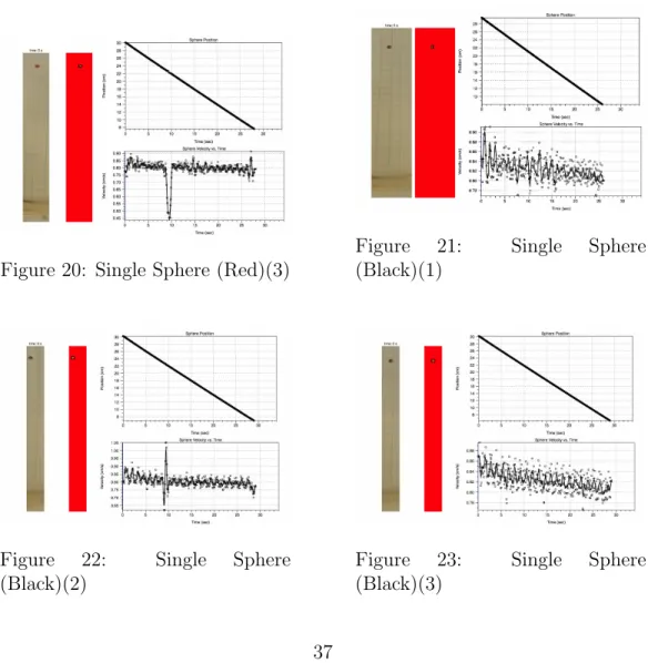
Figure 20: Single Sphere (Red)(3)

Figure 21: Single Sphere (Black)(1)

Figure 22: Single Sphere (Black)(2)

(39)

Figure 24: (Vertical/Red-on-Black/0.10cm)(Red)(1)

Figure 25: (Vertical/Red-on-Black/0.10cm)(Black)(1)

Figure 27: (Vertical/Red-on-Black/2.75cm)(Black)(2)

(40)

Figure 30: (Vertical/Black-on-Red/0.87cm)(Red)(4)

Figure 31: (Vertical/Black-on-Red/0.87cm)(Black)(4)

Figure 32: (Vertical/Black-on-Red/4.02cm)(Red)(4)

(41)

Issues: The focus should had been checked between test. By coloring over the already dried marker on the spheres, the old marker coloration be-came wet and easily be-came off during experiments. After each run, the sphere would have to be cleaned and recolored, making for very poor coloring over-all. In most of the tracking, a glob of corn syrup on the outside of the tank messed up the tracking for several frames creating dramatic jumps in the velocity tracking and the graph. This implies that the tank should be more thoroughly cleaned between experiments. The vertical drops were near im-possible to get to drop tangentially. Likewise, for other vertical drops, the distance couldn’t be controlled for and was calculated post experiment. The retrieving mechanism had a crevice between the spoon, the rod and the duct tape that held the two together. This led to a constant stream of giant bub-bles entering the corn syrup. Like usual, the plastic wrap was hard to get back on without affecting the initial fall of the sphere. More paper towels were needed.

Conclusion: The experiment succeeded in reasonably eliminating the two assumed possibilities of error that the experiment was designed to elim-inate: human error and time measurement issues with interval shooting, but all the same, still produced the frightening discrepancy in experimental ver-sus model. In other words, the error is neither from the measurement tools (unless they are broken or not calibrated correctly) nor from the experi-menters, indicating that we need to look into other possibilities.

15 Issues with the Viscometer and

Alterna-tives

Viscometer Issues

(42)

the corn syrup. This led to the exploration into its behavior around zero (Taylor Expansion) and me switching to Stokes drag. After finding out that the equation wasn’t an issue, we looked into instrumental error. After con-cluding that even that was not substantial enough to account for the error, we thought it may have been experimental [note all the issues in experiment two]. My prediction was that the cameras picture timer was off and wasn’t accurately taking one second interval photos or that I had messed up as an experimenter. So in consequence, experiment three was ran to compensate for this and other possible issues by having multiple experimenters present, and using video recording instead of interval photos. Yet still we had discrep-ancy between the predicted and the experimentally observed. Finally, after beginning a retesting of the devices for error, it struck me how strange it was that there was such a large deviation between even and odd measurement by the viscometer. To elaborate, the viscometer runs multiple measurements by rotating a glass capillary with a gold bead suspended in the to be measured fluid, then tracks the beads descent using electro-conductivity. Using this data, and a standard of calibration, and a density it can measure viscosity. thus measurements are formed in pairings with the starting orientation being the odd measurements (the 1st, 3rd, etc.), and the flipped orientation being the even. So after a quick look into previous data charts, it became apparent that this large deviation of up to 9 Pascal Seconds was non-existent prior to two measurements ran earlier before my measurements where recorded.

From 2008:

(43)

Alternative: Viscosity Cups

While we attempted to fix the viscometer, we needed to find an alterna-tive way to measure the viscosity for experiment three before the corn syrup in the tank begins to evaporate and change viscosity. Adviser Camassa rec-ommended that I try using ”Viscosity Cups”. These are metal cups with different volumes and sized holes in the bottom for different ranges of veloc-ities. After filling them up with the liquid you want to measure, your record the amount of time it takes for the fluid to run out (for the falling stream to have a definite break). Based off of the time and a table, you can retrieve a viscosity.

11/25/2015

Averaging 5 separate measurements from viscosity cup number 5, we aver-aged at 60.13 seconds. The table gave us a measurement of 1401 centiStokes, which with a density of 1.36902 g/cm3_{, gives us 19.18 Pascal Seconds. This}

(44)

Results:

Type Terminal Velocity Predicted Error Single Sphere (Red)(1) 0.795560 0.787463 1.03% Single Sphere (Black)(1) 0.826212 0.787463 4.92% Single Sphere (Red)(2) 0.807280 0.787463 2.52% Single Sphere (Black)(2) 0.808012 0.787463 2.61% Single Sphere (Red)(3) 0.794257 0.787463 0.86% Single Sphere (Black)(3) 0.826110 0.787463 4.91% Double Sphere

(Ver-tical) (Red-on-Black) 0.10cm(Red)(1)

1.208318 1.23117 11.58%

Double Sphere (Ver-tical) (Red-on-Black) 0.10cm)(Black)(1)

1.194725 1.23117 10.33%

Double Sphere (Ver-tical) (Red-on-Black) 2.75cm)(Red)(2)

0.875607 0.89169 8.45%

0.858294 0.89169 6.31%

1.126024 1.12818 12.68%

1.107042 1.12818 10.78%

1.019809 1.02032 11.85%

1.046783 1.02032 14.81%

0.826242 .863185 5.36%

(45)

Amazingly, considering the 12 day separation, these numbers are remark-ably close to what we predicted. Providing more evidence toward a faulty viscometer.

Fixing the Viscometer:

After a couple week span of calling Anton Paar, being told we had a bad belt and needed to send it in for repairs, attempting to schedule with other universities to minimize travel cost for repairman, then lastly fixing the viscometer with the assistance of a technician over phone, we were finally able to both confirm that the viscometer was providing false reading and get it in working order.

16 Dropping Apparatus

To control drop separation and provide precise positioning for different con-figurations I have developed a dropping apparatus:

Objects:

-Disassembled mechanical pencil green plastic casing -Two Doweling Rods

(46)

(47)

Pros: Is a great improvement on retrieval (as opposed to the spoon), punctures the evaporated surface interface without tainting the sphere(s), drops very consistently, is easier to manipulate orientation and separation of spheres, less of a mess for hands.

Cons: Has to be cleaned after each run, requires a separate holding beaker of top layer, it is hard not to tilt tool when dropping (no structure to keep everything aligned in tank).

(Note:Is approximately a three feet long)

17 Experiment Four: Second Re-Test of Two

Identical Spheres in Homogeneous Corn

Syrup

Date:12/15/2015

Problem and Purpose: Although experiment three looked incredible after taking the velocity cups into consideration, we still need two things before we make the big step into a stratified regime: more data points, a viscosity taken from an instrument that is both precise and built to measure at the viscosity of our fluid. In other words, this experiment is just a reas-surance before we continue into the stratified regime.

Materials:

-Small Plastic Cylinder Tank with Diameter of Approximately 10.75cm

-Corn Syrup of Density of Approximately 1.37440g/cm3_{and Viscosity 24}_.₅₁₉₀_{P a.s}

Viscometer Cups, and Density of 1.37537 g/cm3 and Viscosity 26.3997P a.s

Viscometer (12/18/2015) -Camera Mount

-Giant Plastic Spoon for stirring

-Designed Tool for Retrieval and Dropping

≈2.26

(48)

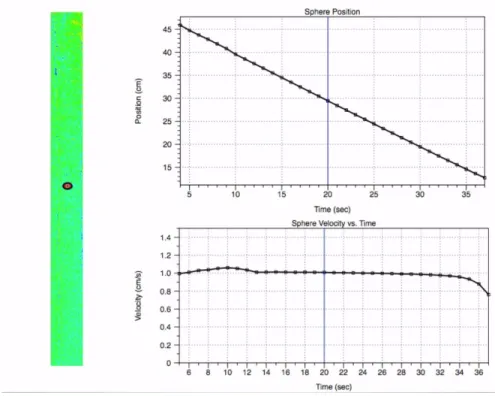
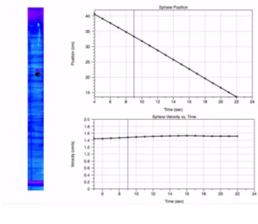
Set-up: Corn syrup from Experiment Three was poured into the metal mixing pot and additional corn syrup was added from the stored containers. It was then stirred for 40 minutes, poured back into the cylinder, covered in two layers of plastic wrap to prevent evaporation, and left over two nights. The day of the experiment, the spheres were recolored with marker, the den-sity was taken, the viscoden-sity was measured with the viscoden-sity cups (with the help of Claudia Falcon), and a sample for the viscometer (still not working at this point) was taken. The camera was mounted, balanced and focused. A large beaker full of corn syrup from the tank that is used for holding the retrieval tool, priming it for the drop, and holding the spheres was put beside the tank. The netal mixing pot is palced beside the tank, full of wa-ter, for cleaning. Lastly, paper towels were procured from the bathrooms. (Note: Viscosity was taken again three days later after viscometer was fixed). Procedure: The experiment consisted of 18 drops, of which, 14 were considered suitable for analysis. An experiment was performed in the follow-ing manner, spheres are submerged in holdfollow-ing beaker. Focus and orientation of camera is checked. Record button is pressed. Tool is submerged in holding beaker, and sphere are sucked up. Tool is lifted from beaker and hand cups bottom to prevent dripping on table and tank. Tool is submerged. Orienta-tion of tool in liquid is checked. Spheres are slowly pushed out and distance adjusted. Slowly tool is removed and I back away as to prevent shadows. I wait for spheres to stop falling, then Stop the recording. Retrieve spheres using tool. Drop spheres in metal pot full of water. Clean tool, then dry tool. Clean spheres under water, then dry spheres. Put spheres into holding beaker. Repeat.

(49)

Type Distance Terminal Velocity Stand. Dev. from Terminal Predicted Error Single Sphere (Red)(1)

NA 0.5763203 0.03101 0.571759 .7915 %

Single Sphere (Black)(1)

NA 0.578095 0.00904 0.571759 1.09601%

Verticle Double Sphere BR(Red)(1)

0.069428 0.8397748 0.01663 0.904367 7.69%

Verticle

Dou-ble Sphere

BR(Black)(1)

0.069428 0.8365177 0.01884 0.904367 8.11%

Verticle Double Sphere (Red)(2)

0.0971035 0.821565 0.02923 0.894898 8.93%

Verticle Double Sphere (Black)(2)

0.0971035 0.8176483 0.02268 0.894898 9.45%

0.236437 0.8101529 0.0260 0.852232 5.19%

0.236437 0.8063606 0.01942 0.852232 5.69%

0.258821 0.7655826 0.03126 0.846182 10.53%

0.258821 0.7649389 0.02393 0.846182 10.62%

0.269877 0.7859402 0.02851 0.843272 7.29%

0.269877 0.7812826 0.02529 0.843272 7.93%

0.40301 0.7037796 0.02845 0.811997 15.38%

0.40301 0.700383 0.01794 0.811997 15.94%

0.841339 0.6991079 0.02829 0.74401 6.42%

0.841339 0.6976924 0.02093 0.74401 6.64%

0.882405 0.693005 0.03190 0.739486 6.71%

(50)

Type Distance Terminal Velocity Stand. Dev. from Terminal Predicted* Error Verticle Double Sphere (Red)(9)

1.07381 0.6862634 0.02646 0.721115 5.08%

1.07381 0.6779655 0.01782 0.721115 6.36%

1.55623 0.6434068 0.02345 0.688587 7.02%

1.55623 0.6424083 0.01964 0.688587 7.19%

1.99998 0.6156543 0.02247 0.668984 8.66%

1.99998 0.611132 0.01884 0.668984 9.47%

2.22849 0.6192461 0.02786 0.661232 6.78%

2.22849 0.6160281 0.01593 0.661232 7.34%

3.31512 0.5912805 0.03625 0.636585 7.66%

3.31512 0.5907453 0.02128 0.636585 7.76%

4.4378 0.5855548 0.02463 0.622195 6.26%

(51)

[p]

(52)

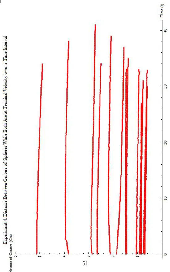
[p]

Figure 35: As predicted by Camassa, the distance between the spheres are relatively fixed with minor variance (This is corroborated by previous

(53)

Figure 36: Single Sphere Red Figure 37: Single Sphere Black

Figure 38: Double Sphere Red 0.069428 (cm)

Figure 39: Double Sphere Black 0.069428 (cm)

(54)

(55)

Figure 50: Double Sphere Red 0.841339(cm)

(56)

(57)

Figure 63: Double Sphere Black 3.31512(cm)

(58)

Issues: The test went well and the only issues, as in previous experi-ments, was the necessity of better tracking and dropping. The tool that is used to drop the spheres does not compensate for the angle between the two spheres. It is still up to the experimenter to perfectly align them coaxially.

Conclusion: The experiment succeeded in providing a clear and definite result for coaxial spheres in low Reynolds, homogeneous fluid. The data looks great plotted, as when error is taken into account, seems completely within reason. It also show the issues with the Kynch prediction, seeming more like an upperbound for the experiment (although a vertical shift well aligns it with the points). With all this said, I think we have a strong enough of an experiment to move into our next regime: sharply stratified solutions.

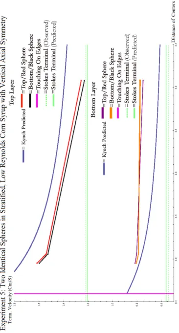
18 Experiment Five: Two Identical Spheres

in Stratified Corn Syrup (NaCl)

Date:12/18/2015

Problem and Purpose: Now we are moving into a stratified regime to act as a basis for our theory and to develop rudimentary observations. This experiment will also give us an understanding of what complications may arise from testing in a stratified regime and how a colored die effects our tracking.

Materials:

-Small Plastic Cylinder Tank with Diameter of Approximately 10.75cm -Top Corn Syrup of Density 1.36133 g/cm3 _{and Viscosity 12}_.₇₀₈_{P a.s}

Vis-cometer

-Bottom Corn Syrup of Density 1.38183 g/cm3 _{and Viscosity 26}_.₆₄₂₇_{P a.s}

Viscometer -Camera Mount -Plastic Wrap -Metal Mixing Pot

(59)

≈2.26

(60)

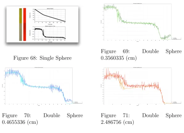
Results:

Type Single Red Red-on-Black (1) Red-Black

Red-on-Black (2) Red-Black

Red-on-Black (3) Red-Black

Distance NA 0.3560335 0.4655336 2.486756

Terminal Velocity Top

1.20654 1.617611 — 1.59913 1.54164 — 1.528434 1.256683 — 1.230643

Stand. Dev. of Terminal Velocity Top

0.02035 0.06656 — 0.01364 0.09729 — 0.01956 0.09803 — 0.01533

Predicted Top

1.218262 1.752060 1.70338 1.39313

Error Top .97% 8.31% — 9.56% 10.49% — 11.45% 10.86% — 13.20% Terminal

Velocity Bot

0.56246 0.80601 — 0.81688 0.78888 — 0.80304 0.77535 — 0.75132

Stand. Dev. of Terminal Velocity Bot

0.00944 0.02346 — 0.01308 0.09700 — 0.01326 0.05993 — 0.01400

Predicted Bot

0.5439585 0.7823 0.760565 0.622036

(61)

(62)

(63)

Figure 68: Single Sphere

Figure 69: Double Sphere 0.3560335 (cm)

Issues: The test should have been performed at an earlier hour in the day. Being around 1am, the experimenter was tired and only able to run the few test he did and was inhibited in performance. Likewise, the interface could have been more gently penetrated by the device, and the dying of the top layer did seem to help much and could have very well, had the opposite effect, making tracking more difficult. Overall a success, and when we run a future test to gather more data points, we can address these issues.

(64)

19 Experiment Six: Re-Test Two Identical

Spheres in Stratified Corn Syrup (NaCl)

Date:1/08/2016

Problem and Purpose: This will be larger more expansive undertak-ing then experiment 5 (similar to how experiment 4 was to experiment 3), providing enough data points to establish a trend and behavior. We will also be using the data gathered from experiment 5 to improve testing and hopefully give us a good data set to begin developing theory.

Materials:

-Small Plastic Cylinder Tank with Diameter of Approximately 10.75cm -Top Corn Syrup of Density 1.38748 g/cm3 and Viscosity 28.8448P a.s Vis-cometer @23.62 Celsius

-Bottom Corn Syrup of Density 1.37718 g/cm3 _{and Viscosity 34}_.₆₅₁₁_{P a.s}

Viscometer @23.62 Celsius -Camera Mount

≈2.26

(65)

full of corn syrup from the tank that is used for holding the retrieval tool, priming it for the drop, and holding the spheres was put beside the tank. The metal mixing pot was placed beside the tank, full of water, for cleaning. Lastly, paper towels were procured from the bathrooms. The corn syrup mixed with table salt was poured into the tank first. Then, with the help of Claudia Falcon, the next layer of corn syrup, mixed with water, was poured into the tank, slowly, so as to create a sharp stratification. The ruler was stuck to the side of the tank via putty, the outside surface of the tank cleaned, and the liquid covered in plastic wrap.

Procedure: The experiment consisted of 12 drops, of which 6 were con-sidered suitable for analysis. An experiment was performed in the following manner. First, the spheres are submerged in the holding beaker. The focus and orientation of the camera is checked. Record button is pressed. The tool is submerged in holding beaker, and the spheres are sucked up. The tool is lifted from beaker with my hand cupping under the tool as to prevent corn syrup dripping on the table or the tank. The tool is submerged a few cen-timeters under the surface. Orientation of the tool in the liquid is checked. The spheres are slowly pushed out and distance adjusted. Slowly, the tool is removed and I back away as to prevent shadows. I wait for the spheres to stop falling, then stop the recording. Retrieve spheres using tool, being very careful to minimize damage to the interface. Drop spheres in a metal pot full of water. Clean the tool,and then the dry tool. Clean the spheres under water, then dry spheres. Put the spheres into a holding beaker. Repeat.

Results/Issues/Conclusion:

(66)

ex-periment, this indicates something related to the only two parameters that changed, the density and the viscosity. Lastly, I have a hunch the reduction in approach distance is strongly related to the viscosity since the difference in top and bottom viscosity is large in experiment 5 (difference of approx. 14 Pa.s) and small in experiment 6 (difference of approx. 6 Pa.s). Whereas the difference in density was approximately .01 in experiment 5 and .02 in ex-periment 6. Since the change in viscosity seems more dramatic, I’m inclined to see it as the main contributor.

20 Experiment Seven: New Salt, Two

Identi-cal Spheres in Stratified Corn Syrup (KI)

Date:1/26/2016

Problem and Purpose: As noted in experiment 6, this will be larger more expansive undertaking then experiment 5 (similar to how experiment 4 was to experiment 3), providing enough data points to establish a trend and behavior. We will also be using the data gathered from experiment 5 to improve testing and hopefully give us a good data set to begin develop-ing theory. Also, with the advice of Professor Camassa, we will be usdevelop-ing KI (Potassium Iodide) to create a larger density separation to see a more dramatic entrainment effect.

Materials:

-Small Plastic Cylinder Tank with Diameter of Approximately 10.75cm -Top Corn Syrup of Density 1.37781g/cm3 _{and Viscosity 30}_.₇₇₄₄₀₀_{P a.s}

Vis-cometer @23.05 Celsius

-Bottom Corn Syrup of Density 1.41578g/cm3 and Viscosity 26.494800P a.s

(67)

≈2.26

Set-up: Corn syrup from storage was poured into the metal mixing pot. After 40 minutes of mixing, the density was taken and the corn syrup poured into a 2000 ml container and covered with plastic wrap. After cleaning the pot corn syrup from storage was added in along with approximately 55 ml of KI salt. After 40 minutes of stirring, taking a density and looking into the solubility of KI in water, I inferred that another 50 ml of KI would be safe to mix into solution without fear of over saturation. Then, after 40 minutes of mixing, the corn syrup was poured into a 2000 ml container and covered with plastic wrap. The solution was left for five days. Then on the day of the experiment, the viscosity and density of both corn syrups was gathered. The spheres were recolored with marker. The camera was mounted, balanced and focused. A large beaker full of corn syrup from the tank that is used for holding the retrieval tool, priming it for the drop, and holding the spheres was put beside the tank. The metal mixing pot was placed beside the tank, full of water, for cleaning. Lastly, paper towels were procured from the lab. The corn syrup mixed with KI was pored into the tank first. Then, with the help of Claudia Falcon, the next layer of corn syrup was poured into the tank, slowly, so as to create a stratification. The ruler was stuck to the side of the tank via putty, the outside surface of the tank cleaned, and the liquid covered in plastic wrap.

(68)

Results*:

Type Distance Terminal

Velocity)

Stand. Dev. from Terminal

Predicted

Single Red 1 NA 0.5129926 — 0.5554601 0.009147 — 0.008163 0.485941 — 0.540139

Single Black 1 NA 0.5091437 — 0.5535152 0.02646 — 0.013252 0.485941 — 0.540139 Double Red-on-Black 1 Red

1.84107 0.5666663 — 0.5739903 0.011689 — 0.01015 0.680448 — 0.756339 Double Red-on-Black 1 Red-on-Black

1.84107 0.5690487 — 0.5792552 0.011062 — 0.010401 0.680448 — 0.756339 Double Red-on-Black 2 Red

0.57177 0.7407136 — 0.7897054 0.018860 —0.018160 0.900967 — 1.00145 Double Red-on-Black 4 Red-on-Black

(69)

Double Red-on-Black 5 Red

2.28915 0.5553703 — 0.5778868 0.011431 —0.010663 0.655545 — 0.728659 Double Red-on-Black 6 Red

2.04872 0.5636054 — 0.5791662 0.016237 —0.012141 0.667612 — 0.742072 Double Red-on-Black 6 Red-on-Black

2.04872 0.5661987 — 0.5792844 0.012655 —0.015428 0.667612 — 0.742072

(70)

(71)

(72)

(73)

Figure 75: Single Sphere

(74)

(75)

Issues: The test was a success and the only issues, as in previous ex-periments, is the constant need for better tracking and dropping. Also, the deviation from predicted terminal was higher then expected, but may be due to temperature variations. It would be nice to pin down why exactly the pre-dicted is slower then what we observe in almost every experiment. Lastly, at the advice of Dr. Camassa, to create a simpler scenario to observe behavior and to have data tat can be run in Claudia’s simulation, I will need to get nearly identical viscosity.

Conclusion: The experiment providing some amazing conclusions. First, and foremost, the spheres are now separating from each other. Is this a con-sequence of the different salt? Second, we are noticing a very consistent behavior/shape on the distance plots. Can we predict that? The third and least understood observation is that within a certain range, the top sphere is going slower then the bottom sphere. Why are they flip flopping?. This needs to be looked into further.

21 Experiment Eight: Test Two Identical Spheres

in Stratified Corn Syrup (KI) with

Simi-lar Viscosity

Date:2/10/2016

(76)

simulation code for single particle through a stratified fluid require identi-cal viscosity. So by satisfying this, we will be able to simulate and test our experiments against those simulations. As before, more data is always a good thing, and since we are adding water to the top layer to create similar viscosity, the density separation will be greater, allowing for more dramatic stratification.

Materials:

-Small Plastic Cylinder Tank with Diameter of Approximately 10.75cm -Top Corn Syrup of Density 1.42608 g/cm3 _{and Viscosity 26}_.₇₉₄₄_{P a.s}

Vis-cometer @23.05 Celsius

-Bottom Corn Syrup of Density 1.37560 g/cm3 _{and Viscosity 2641}_.₉₄_{P a.s}

≈2.26

(77)

(78)

(79)

Procedure: The experiment consisted of 11 drops of the 2.6 density spheres, of which, none were considered suitable for analysis. An experiment was performed in the following manner. First, the spheres are submerged in the holding beaker. The focus and orientation of the camera is checked. Record button is pressed. The tool is submerged in holding beaker, and the spheres are sucked up. The tool is lifted from beaker with my hand cupping under the tool as to prevent corn syrup dripping on the table or the tank. The tool is submerged a few centimeters under the surface. Orientation of the tool in the liquid is checked. The spheres are slowly pushed out and distance adjusted. Slowly, the tool is removed and I back away as to pre-vent shadows. I wait for the spheres to stop falling, then stop the recording. Retrieve spheres using tool, being very careful to minimize damage to the interface. Drop spheres in a metal pot full of water. Clean the tool,and then dry the tool. Clean the spheres under water, then dry spheres. Put the spheres into a holding beaker. Repeat.

(80)

(81)

Unfortunately, after attempting to analyze the videos, it became obvious that there was a linear stratification in the bottom layer. I theorize that the undissolved salt (since it was grounded), had lied in the bottom of the tank and then, between the initial mixing and test day, slowly dissolved into the bottom. This then created a lower higher density in the bottom of the bottom layer.

22 Experiment Nine: Re-Test Two Identical

Spheres in Stratified Corn Syrup (KI)

Date:2/27/2016

Problem and Purpose: Experiment 8 was a failure that still resulted in some interesting observations. Regardless, we still need similar viscosity. As noted before, this will eliminate some variables, making understanding the basic behavior easier and satisfies the parameters for Claudia’s simulation. Also as noted, more data is always a good thing, and since we are adding water to the top layer to create the similar viscosity, the density separation will be greater, allowing for more dramatic stratification. Lastly, and most importantly, this will provide the parameters necessary to apply the obser-vations made on the velocity sphere from a UNC student

Materials:

(82)

Vis-cometer @22.48* Celsius

-Bottom Corn Syrup of Density 1.37419 g/cm3 and Viscosity 26.9517P a.s

Viscometer @22.48* Celsius -Camera Mount

-Sphere Red, Radius(cm)=0.296545, Density(g/cm3)_≈2.26 -Sphere Black, Radius(cm)=0.296545, Density(g/cm3₎

≈2.26

Set-up: After borrowing a mortar and pestle from the neighboring lab, is spent 45 minutes grinding 160 ml of granualted KI. corn syrup from storage was poured into the metal mixing pot. After 40 minutes of mixing, the den-sity was taken and the corn syrup poured into a 800ml container and covered with plastic wrap. After cleaning the pot corn syrup from storage was added in along with approximately 120 of KI salt. After 40 minutes of stirring, I took the density and viscosity of both. Then the corn syrup mixed with KI was poured into the experimental tank and covered with plastic wrap. The solution was left for four days. Then on the day of the experiment, the viscosity and density of both corn syrups was taken again. The spheres were recolored with marker. The camera was mounted, balanced and focused. A large beaker full of corn syrup from the tank that is used for holding the re-trieval tool, priming it for the drop, and holding the spheres was put beside the tank. The metal mixing pot was placed beside the tank, full of water, for cleaning. Lastly, paper towels were procured from the lab. Then the next layer of corn syrup mixed with water was poured from the 800ml container into the tank, slowly, so as to create a stratification. The ruler was stuck to the side of the tank via putty, the outside surface of the tank cleaned, and the liquid covered in plastic wrap.

Thesis

The Mathematics of Sinking

Through Sharply Stratified

Liquids

An Experimental Approach with Spheres

The Mathematics of Sinking Through

Sharply Stratified Liquids

An Experimental Approach

Jacob Dylan Bruney

Abstract

1

Table of Contents

Contents

2

Introduction

3

Literature Review

4

Terminal Velocity of a Single Sphere in Low

Reynolds Free Space

5

Elementary models to predict two spheres

falling:

6

Developing a Drag Coefficient for Finite

Reynolds

7

Terminal Velocity of a Single Sphere Finite

Reynolds

8

Taylor Approximations:Morrison’s

Coeffi-cient As Reynolds Approaches Zero

9

Boundary Condition

10

Experiment Setup and Analysis:Visual

11

Experiment One: Two Identical Spheres

in Homogeneous Water

12

Experiment Two: Two Identical Spheres

in Homogeneous Corn Syrup

13

Error Propagation

14

Experiment Three: Re-Test Two

Identi-cal Spheres in Homogeneous Corn Syrup

15

Issues with the Viscometer and

Alterna-tives

16

Dropping Apparatus

17

Experiment Four: Second Re-Test of Two

Identical Spheres in Homogeneous Corn

Syrup

18

Experiment Five: Two Identical Spheres

in Stratified Corn Syrup (NaCl)

19

Experiment Six: Re-Test Two Identical

Spheres in Stratified Corn Syrup (NaCl)

20

Experiment Seven: New Salt, Two

Identi-cal Spheres in Stratified Corn Syrup (KI)

21

Experiment Eight: Test Two Identical Spheres

in Stratified Corn Syrup (KI) with

Simi-lar Viscosity

22

Experiment Nine: Re-Test Two Identical

Spheres in Stratified Corn Syrup (KI)