1
The Impact of State Government Partisan Composition on Health Outcomes
through Taxation and Healthcare Spending
Honors Thesis
Paul Archimedes Kushner April 2017
Economics Department
The University of North Carolina at Chapel Hill Thesis Advisor: Professor Patrick Conway
Faculty Advisor: Professor Klara Peter
Approved: ______________________________________________ Professor Patrick Conway
A further thanks to all the students of the economics honors thesis program who gave me much
appreciated feedback throughout the crafting of this paper as well as all my economics
instructors at the University of North Carolina at Chapel Hill. A special added thanks to Michael
Aguilar who first introduced me to economics research and has most influenced my time as an
2 I. Abstract
This paper examines the relationship between the partisan composition of state
governments and healthcare in that state. It first shows the theoretical conditions which impact taxation and healthcare spending policies. This theory supports the notion that divided
governments produce better healthcare outcomes for individuals than unified state governments. These theoretical conditions are then tested empirically in four iterations. The first iteration considers the direct relationships posited by the theoretical model as stand-alone equations. The second iteration adds variables designed to control for demographic and economic conditions in each state and evaluates the impact of a state’s decision to expand Medicaid. The third iteration of these relationships is a simultaneous estimation of the first iteration. Simultaneous estimation addresses the existence of several variables as both dependent variables in certain equations and independent variables in others. The fourth iteration simultaneously estimates the relationships with the inclusion of state level control variables and an analysis of whether or not a state chose to expand Medicaid. The theoretical results suggest that health outcomes can be altered on a short time horizon by state governments through policy. However, this assertion fails to hold up when properly modeled and the results suggest that state governments do not have a discernable effect on the health outcomes of their citizens on Medicaid. The only finding of the theoretical model that holds up to rigorous econometric examination is that government complexion significantly impacts the tax rate in a state as unified state governments increase taxes in the states they control.
II. Introduction, Background Information, Motivation and Contribution
3
from 2000-2014. Ultimately, this research focuses on health outcomes for Medicaid enrollees as determined by the taxation and health policies of state governments. The political complexion is also crucial in determining the extent of healthcare coverage in each state. Healthcare coverage refers to the Medicaid program in each state. From state level healthcare spending and coverage under Medicaid, this research will then examine the effect on individuals on Medicaid in terms of their health outcomes.
A key motivating factor for this study was the fact that the topic of income inequality has increasingly permeated American politics in both parties. Correspondingly, income inequality has emerged as an economic topic of study. At each stage of this discussion, the focus has been on the federal government’s power to either correct or unintentionally exacerbate income inequality through various actions, particularly tax policy and spending on various programs. This focus on the federal government has overlooked the role of state governments. This paper sets up a framework to review and then examine the effects of the complexion of state
governments on health outcomes within the state. Income inequality is not examined as an explicit portion of the relationships between political complexion and health outcomes, but it does feature in the models when accounting for the conditions in each state.
Republicans and Democrats have each talked about income inequality as a pressing national issue throughout the past few years. At the same time, the federal government has been divided and enacted very few policies. With that as a backdrop, state governments have been incredibly active over the past few years, passing far more legislation that the federal
government.1,2 As such, I wanted to explore how states have approached inequality since the year
1 Govtrack. (2017)
4
2000. This research evolved from that initial desire and quickly incorporated healthcare as the principal lens through which to analyze this topic. From there it was quickly obvious that examining Medicaid and various factors relating to Medicaid would both be a unique topic, but also highlight how a state government could make specific choices relating to the healthcare outcomes of its citizens and whether or not this changed in states with different levels of income inequality.
This paper focuses on healthcare coverage and health outcomes. This is due to the fact that states can set their own policies on healthcare through the Medicaid program. In the United States, the federal government sets a great deal of the health policy, but cedes the states a great deal of flexibility in how to structure their Medicaid programs within each state. Medicaid is a public insurance program which covers the healthcare of poor citizens in the United States. Medicaid eligibility is determined on a state—by—state basis, with some baseline requirements for eligibility determined by the federal government. These requirements are both income-based and condition-based. All children through age 18 in families with an income below 138% of the federal poverty line, pregnant women with income at or below 138% of the federal poverty line, and some seniors and disabled people are eligible for the program. States have a great deal of freedom in determining whom else they choose to cover under the Medicaid program. Under the Affordable Care Act, some states have expanded Medicaid to cover all adults with incomes up to 138% of the federal poverty line and have adopted other changes to increase eligibility. Other states have declined to expand Medicaid under the Affordable Care Act which highlights the drastic impact that a state government can have on Medicaid in the state. The variation in
5
which services to cover under the Medicaid program, which further highlights the importance of state governments in determining healthcare across the nation.3
To further break down and analyze how each state’s decisions and preferences impact the Medicaid program in each state, the states Alabama, California and North Carolina will be considered as case studies. Each of these states has taken a different approach to Medicaid and these approaches outline how different each state’s program can be. Alabama has a simple structure for eligibility and benefits. In Alabama, the state government declined to expand Medicaid and as such not many people are eligible for the service. In Alabama, those on Medicaid are children in families with income up to 141% of the federal poverty line, pregnant women with incomes up to 141% of the poverty line and parents with incomes up to 13% of the federal poverty line.4 Further, individuals with incomes that do not exceed $755 per month ($1,123 for a couple) are eligible for Medicaid in Alabama if they are 65 or older, blind or disabled.5 Within its Medicaid program, Alabama imposes strict caps on the number of times a year that an individual can receive health services. The program limits enrollees to 14 doctor visits each calendar year and three outpatient hospital visits. Another quota embedded in the program is the cap on eye care services stating that enrollees can only have eye exams and eye glasses covered once every three years. The state’s program also features multiple differences in services covered depending on the age of the enrollee. For instance, dental services are only covered for enrollees under the age of 21 and psychiatric hospital services are available to enrollees under the age of 21 and over the age of 65.6 Each facet of Alabama’s Medicaid program is determined by the state government. The eligibility thresholds are set by the state
3 Center on Budget and Policy Priorities. (2017) 4 HealthInsurance.org. (2017). “Alabama Medicaid”
5 State of Alabama. (2017). “Medicaid Income Limits for 2017”
6
government as are the services covered and for which enrollees those services are provided. The program in Alabama is not restarted each year anew, rather it is augmented gradually over the time period. This paper will theorize that the change in the government complexion in the state over the time horizon of 2000-2014 will alter the state’s Medicaid program and these changes have observable consequences on taxation, the size of the state’s Medicaid subsidy, Medicaid coverage, and health of their Medicaid enrollees.
The state of California faces similar choices to the state of Alabama when deciding how to construct its Medicaid program but has made radically different decisions as to how to
structure it. In California those eligible for Medicaid are children from birth through age 18 with family incomes of up to 266% of the federal poverty line, pregnant women with incomes up to 213% of the federal poverty line, and adults with or without children with incomes up to 138% of the federal poverty line. These eligibility requirements are markedly different from the requirements in Alabama with the most notable difference being the fact that Alabama limits eligibility among nonelderly adults to those with incomes less than or equal to 13% of the federal poverty line for parents while California allows all adults independent of their parental status to enroll in the program if their income is less than or equal to 138% of the federal poverty line.7 The differences in eligibility standards come directly from decisions that the state government of California has made. The state government, influenced by partisan complexion, chose to adopt these eligibility standards as well as to accept a mostly federally funded expansion of Medicaid. The benefits of Medicaid in California are also significantly different than those in Alabama. In California enrollees have access to a generous set of services as medically necessary without the quotas seen in Alabama. California covers all medically necessary physician services including
7
inpatient and outpatient care. Furthermore, the state covers all hospitalization services with no annual limit on services provided including any necessary organ and tissue transplantation
services. In an additional clear contrast to Alabama’s program California provides dental benefits to all enrollees ranging from basic preventative care to emergency dental services to dentures while Alabama refrained from offering such services to enrollees. California also offers eye exams once every two years as opposed to Alabama offering those services every three years.8 Once again, the state’s decisions have a clear impact on the construction of the Medicaid program. California has opted to extend a far more generous benefits package to its Medicaid participants and its participants face much more generous admissions criteria. In determining both eligibility criteria and benefits offered, the state government of California has made very different choices compared to the state of Alabama.
The final state whose Medicaid program will be considered as a case study is North Carolina. As a student at the University of North Carolina at Chapel Hill, the decisions of the state government of North Carolina are of particular interest to me. North Carolina, as in
Alabama, opted to decline to expand Medicaid under the Affordable Care Act. The state of North Carolina has confined Medicaid eligibility to the blind, aged, disabled, parents with dependent children with household incomes up to 45% of the federal poverty line, children with family incomes less than or equal to 211% of the federal poverty line, and pregnant women with incomes up to 196% of the federal poverty line.9 These standards are more restrictive than California but more generous than the standards for eligibility in Alabama. This intermediate standard of eligibility highlights the fact that states face a clear choice when setting eligibility guidelines. States have a whole spectrum of eligibility options available to them when they set
8
eligibility guidelines. The eligibility criteria a state chooses to set are decisions that each state government must make when structuring their Medicaid program.
North Carolina has a benefits system that is very similar to the Alabama program. In North Carolina, benefits are tied to age, income, and health status (blind, disabled, etc.). The Medicaid benefits that a person is entitled to are not universal like in California; instead, depending on where on the spectrum of eligibility an individual is, their benefits change with their individual status and characteristics. An illustrative example of this phenomenon is once again seen in the dental benefits that a person receives. In North Carolina, Medicaid only covers dental care for children under the age of 21.10 The coverage under Medicaid in North Carolina is more conservative on benefits, and is much more similar to Alabama’s system than California’s. However, the state has elected to adopt more generous admissions criteria than Alabama which showcases the fact that even though states can have similar benefits covered by their Medicaid programs, their decisions on who is covered by Medicaid are equally important to the actual benefits offered. These decisions on eligibility and benefits offer clear points of contrast between the states which this study theorizes results in empirically observed relationships between
government complexion and a host of other factors related to Medicaid in the states.
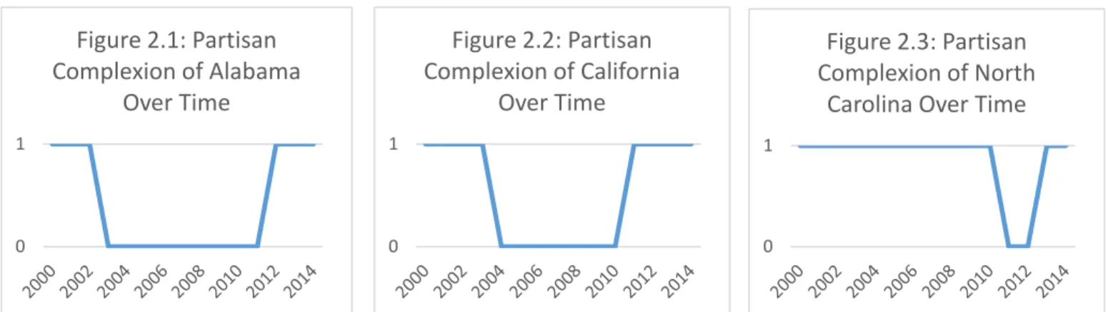
These states not only differ in the benefits that they offer to their Medicaid enrollees, but also in their government complexions over the course of the sample, the years 2000-2014. Each state experiences both divided and unified state government during the sample period. The three figures below display how this study will treat government complexion.
Figures 2.1-2.3:
9
Note: These figures highlight how the partisan complexion of each state over time. This is a dummy variable, a value of 1 represents a unified government while 0 represents a divided government.
The partisan complexion of each state government is a dummy variable. Therefore, in the above figures, the years with a value of one are the years where the state has a unified
government while the times with a divided government are represented with a value of zero. It should also be noted that while these three states which are examined in this Medicaid case study all have graphs of a similar shape, there is a much wider amount of variety when the entire nation is examined later in this paper. The figures show that Alabama has a divided government the most frequently, during 60% of the sample. California has unified government slightly more frequently, 53.3% of the time, the state has a unified government. North Carolina rarely has a divided government during the sample period, with a unified government occurring 86.6% of the time. This research therefore looks at how government complexion can act as a driving force behind the health outcomes and coverage of its citizens through the policy choices of a state with a focus on the decisions the state makes on healthcare spending and taxation. This research attempts to explore the outcomes of that flexibility to determine if partisan government complexion has any impact on healthcare coverage and outcomes for a state’s citizens.
This research is a fairly unique contribution to existing literature. To date, there have been no significant examinations of state level policies on healthcare outcomes. Most economic analysis looks at national or county level statistics. By pursuing this type of research, state
0 1
Figure 2.3: Partisan Complexion of North
Carolina Over Time
0 1
Figure 2.1: Partisan Complexion of Alabama
Over Time
0 1
Figure 2.2: Partisan Complexion of California
10
government choices are typically neglected. Medicaid is another frequently researched topic, but typically this research focuses on the idiosyncrasies of the program and its effects on various individuals. There is also a significant amount of research devoted to how Medicaid works in individual states. However, there is much less research on Medicaid coverage across states. There is a further dearth of research on political complexion. Political complexion of state legislatures is primarily studied in political science rather than in economics. Even then, it is rarely used as an independent variable, but rather a dependent variable. This research is therefore unique on several fronts, filling in gaps by providing a framework for how to investigate state level effects on the health outcomes of its citizens. This is also a new application of data from the Centers of Medicare and Medicaid as well as the Current Population Survey. The remainder of this paper will proceed in six parts, a literature review, thesis and theoretical model, empirical model, results and analysis, conclusion and bibliography. There is also an appendix containing data tables and equations mentioned in the text.
III. Literature Review
“North Carolina’s Employment Record: What role did Unemployment Insurance Reform play?” and “Poverty in North Carolina since 2000: Structural and Cyclical Components” by Dr. Patrick Conway are two of the few examples in current literature of state level studies of policy. Each of these papers deal with factors which features prominently in this research; though not directly, they establish analytical frameworks which are useful for this analysis. North
Carolina’s Employment Record looks at the effect of state level policy decisions on individuals, a key component of this research. Poverty in North Carolina looks at a single state, North Carolina, at the county level. This is different than the analysis in this study as this study
11
level poverty and provided an important framework for looking at the poverty component of this analysis.
The implications of state partisan composition are explored in Robert Jay Dilger’s 1998 paper “Does Politics Matter? Partisanship’s Impact on State Spending and Taxes, 1985-95”. This analysis covers a time period significantly before the timeframe examined in this study, but this paper is an important examination of partisan composition. The critical finding of this paper is the fact that economic factors control state spending and that partisan complexion of states did not have a significant impact on most levels of spending. This paper looked at data from 1985-1995 and looked explicitly at political affiliation rather than the question of unified versus divided government. Furthermore, the paper looked specifically at education in terms of
spending and separated the governorship from the state legislature when looking at complexion. My research, significantly differs in those aspects from the Dilger paper. The most important difference between that analysis and the research presented in this paper is the fact that Dilger’s research was conducted from 1985-1995. Since then, the political ideology of the country has shifted substantially. Additionally, the Medicaid program did not exist at the state level when Dilger wrote his analysis. This paper will almost exclusively focus on Medicaid and therefore has substantially different points of emphasis.
12
13
of the determination of some of the independent variables. When modeling the state’s welfare, the size of the Medicaid subsidy and percent of the population of the state below the poverty line are each crucial independent variables. This paper provided the framework for including these in the model since the paper explored how they impact the well-being of a state.
The other critical paper is David Cutler and Jonathan Gruber’s "The Effect of Medicaid Expansions on Public Insurance, Private Insurance, and Redistribution." This paper examines the evolution of Medicaid over time. Specifically, it looks at the ways in which the various expansions of Medicaid impact how people receive healthcare coverage as well as how the various benefits reach people below and around the eligibility thresholds. The paper finds that the structure of Medicaid expansions greatly alters the impact of the expansion. States operate Medicaid within federal guidelines which give the states wide latitude in determining individual eligibility requirements as well as the services covered by the program. The authors note this and its impact upon their findings, as the different state eligibility thresholds determine who is
14
no matter if they are barely eligible for the program or if their income is well below the poverty thresholds. As a future alternative, the authors advocate for enrollees in the program receiving a larger subsidy if they are poorer and a smaller subsidy if they are wealthier. The paper is relevant to the research presented in this paper as it explores the structure of and decision making process around Medicaid. This analysis will heavily feature Medicaid, its size and the decisions
individuals make around enrollment in that program. As such, it is important to examine
literature on the structure of the program and how that structure effects enrollment. This paper is particularly prescient in its observation of the importance of the size of the subsidy enrollees receive. A critical part the analysis presented in the following sections will be the actions of individuals on the fringe of Medicaid eligibility. This paper notes that individuals barely eligible for the subsidies still receive the full value of the benefit and that benefit’s deterrent to those individuals seeking private insurance coverage. Essentially, the Medicaid subsidy’s size is fixed for all people no matter where on the spectrum of eligibility an individual finds themselves. The fixed size of the subsidy prominently features in the theoretical model in the utility calculations. The authors also note how this transfer away from private insurance is a wealth transfer to these poor families. Both of these facets of Medicaid are important to the analysis in the following sections and this paper establishes a robust framework within which this type of analysis can be done. The key shortcoming of the extant literature which this study will confront is the paucity of rigorous studies of the impact of state governments on Medicaid. There is a further lack of any study of partisan complexion’s impact on these issues.
IV. Thesis, Definitions and Theoretical Model
15
Divided state government refers to the partisan complexion of each state’s legislature and governorship. The partisan complexion refers to which political party controls each part of the state government. All the states in this study possess a bicameral (i.e. two body) state legislature and a governorship. All of these states have partisan offices in both their legislative and
executive branch, that is, when a candidate runs for office they must declare their party
affiliation. After these elections, control of each legislative chamber is determined by whichever party can form a majority out of its members. Partisan control of the governorship is determined by the governor’s political affiliation. Taken together it can be determined if the state has divided or unified government. If one party has majorities in both chambers of the legislature and
16
compromise between the parties which theoretically has a positive benefit for poor citizens. Taken together, the thesis is that divided state governments improve health outcomes of the Medicaid enrollees in states compared to unified governments.
The complexion of the state governments refers to the partisan makeup of the executive branch and legislative branch of state governments. Each state has a similarly constructed executive branch with a governor possessing similar powers and all states except Nebraska have a bicameral legislature. The lack of a partisan state legislature in Nebraska resulted in the dropping of all Nebraska-based data in this analysis.
The following is a table of political complexion by state over the course of the sample: Table 4.1 The Average Political Complexion of Each State from 2000-2014:
State
Political Complexion
Mean State
Political Complexion
Mean
Alabama 0.400 Montana 0.333
Alaska 0.467 Nebraska 0.000
Arizona 0.533 Nevada 0.000
Arkansas 0.467 New Hampshire 0.533
California 0.533 New Jersey 0.533
Colorado 0.667 New Mexico 0.533
Connecticut 0.267 New York 0.400
Delaware 0.467 North Carolina 0.866
Florida 1.000 North Dakota 1.000
Georgia 0.867 Ohio 0.733
Hawaii 0.467 Oklahoma 0.400
Idaho 1.000 Oregon 0.533
Illinois 0.800 Pennsylvania 0.467
Indiana 0.267 Rhode Island 0.267
Iowa 0.333 South Carolina 0.800
Kansas 0.467 South Dakota 1.000
Kentucky 0.000 Tennessee 0.400
Louisiana 0.467 Texas 1.000
Maine 0.800 Utah 1.000
17
Massachusetts 0.533 Virginia 0.133
Michigan 0.467 Washington 0.800
Minnesota 0.133 West Virginia 0.933
Mississippi 0.467 Wisconsin 0.467
Missouri 0.333 Wyoming 0.467
Note: The above table contains information on the government complexion of each state throughout this time period. The variable is a binary dummy variable where every value is a one or a zero. Therefore the mean shown in this table is the expected value of the government complexion in each state at any point during the entire sample.
This table highlights the vast variety of state government complexions seen since 2000. In this dataset, a unified government is shown by having a value of one while a divided
government has a value of zero. A state is given a value for complexion each year so the mean is the average of the state’s complexion for all years of the sample. Since this variable has binary outcomes, each state with a non-integer value for their mean highlights how there have been changes in government complexion over time since the data reported above is the average seen for each state over the entire time period (2000-2014). In fact, very few states have had a divided government or a unified government for every year in the sample. Instead states see the
complexion of their state governments change over the course of the sample. The wide variation seen in government complexion is ideal for this analysis as it means that there are many
observations with both unified and divided governments which increases the strength of the empirical model.
Taxation is another critical aspect addressed in this paper. For the purpose of this
research, state-level taxation will be defined as the average tax rate that each state imposes on its citizens. Each state collects tax revenues in a unique way. Some states rely on a taxation
18
is calculated by taking the total tax revenue that the state collects each year and then dividing it by the state’s population. From this per capita tax revenue value, the tax rate is calculated by dividing per capita tax revenue by the per capita income in a state.
From the examination of taxes and the complexion of the state government, this research will then examine how the state government approaches healthcare spending on the poor. For the period under examination, this will be the amount of money that the state spends on Medicaid. The amount of money the state spends on Medicaid will not include any of the money allocated to the state from the federal government, but rather just the money that the state has collected in taxes and then spends on Medicaid. This is an important distinction because a large portion of funding for Medicaid comes from the federal government rather than the state governments. Since this research and analysis will focus on the impact of state governments, the federal money must be excluded from the analysis. Therefore this research will only consider Medicaid
spending that comes from the state directly as appropriated by the state legislature as a share of income.
19
healthcare and enrollment in Medicaid which enables the construction of the healthcare
outcomes variable. There is a potential source of error introduced into the model at this point as the health status variable is not absolute since it is a measure from one to five. To further refine this variable, the factor included in this analysis will be the percent of a state’s citizens who report a health status of either one or two which is defined as the “bad health” variable. Further mitigating the error in this term is the fact that the data is from the Current Population Survey which reaches thousands of individuals in each state. Despite the fact that the variable has this potential source of error, this still corresponds to the best dataset that could be used for this analysis since it measures everything that is needed for the analysis with thousands of observations in each state.
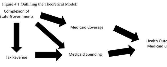
To encapsulate all this in an outline, the following figure roughly displays the theoretical model: Figure 4.1 Outlining the Theoretical Model:
As the figure shows, the complexion of state governments directly affects taxation policy, and together these impact state level healthcare spending on Medicaid. Complexion also impacts Medicaid coverage. Healthcare spending then impacts health outcomes with Medicaid coverage also playing a significant role in determining the health outcomes for Medicaid enrollees. It is important to note here that government complexion does not impact the health outcomes of
Complexion of State Governments
Tax Revenue Medicaid Spending
20
(1)
Medicaid enrollees directly; rather, the impact of partisan complexion on outcomes is seen within the impact that government complexion has on Medicaid coverage and Medicaid spending and then those two factors each impact health outcomes for Medicaid enrollees.
For the empirical framework to reflect this theory, it is important to keep the relationships theorized in the overall context of decisions made by both the state and the individual. In taking this approach, both the state governments and the individuals are treated as utility maximizers. For the individuals, they are governed by an equation that looks like the following Lagrangian with the premise that they will each try to maximize their individual utility (individual subscripts are omitted for simplicity, the assumption is that this equation governs all individuals, the first product is the utility function for the representative individual):
𝐿𝑎𝑔𝑟𝑎𝑛𝑔𝑖𝑎𝑛 𝑓𝑜𝑟 𝑈(𝑐, 𝑙, ℎ) =
𝑐𝑡𝛼∗ (𝐿
𝑡− 𝑙𝑡)(1−𝛼−𝛽)∗ ℎ𝑡𝛽 + 𝜇(𝑤𝑡∗ 𝑙𝑡∗ (1 − 𝜏𝑡) − 𝑃ℎ,𝑡∗ ℎ𝑡− 𝑃𝑐,𝑡∗ 𝑐𝑡)
Where 𝜇 is a Lagrangian multiplier and 𝛼 and 𝛽 are positive with a sum less than one. The consumption for the individual is 𝑐𝑡, the healthcare the individual consumes is ℎ𝑡, the wage earned is 𝑤𝑡, 𝐿𝑡 is the total hours an individual has available while 𝑙𝑡 is number of hours worked, the tax rate is 𝜏𝑡, and the price of healthcare and consumption are indicated by 𝑃𝑐,𝑡and 𝑃ℎ,𝑡 respectively. The price of consumption goods, 𝑃𝑐,𝑡, is not observed and is assumed to be one for both simplification and illustrative purposes to index the price of healthcare relative to the price of consumption goods. Therefore, the individual is subject to the following budget constraint:
𝑤𝑡∗ 𝑙𝑡∗ (1 − 𝜏𝑡) = 𝑃ℎ,𝑡∗ ℎ𝑡+ 𝑃𝑐,𝑡∗ 𝑐𝑡= 𝑃ℎ,𝑡∗ ℎ𝑡+ 𝑐𝑡
This leads to the following first order conditions which focus on the three choices that the individual makes:
21
𝑑𝐿
𝑑𝑐𝑡 = 𝛼𝑐𝑡
𝛼−1∗ (𝐿
𝑡− 𝑙𝑡)1−𝛼−𝛽∗ ℎ𝑡𝛽− 𝜇 = 0
𝑑𝐿 𝑑𝑙𝑡
= −(1 − 𝛼 − 𝛽) ∗ 𝑐𝑡𝛼∗ (𝐿𝑡− 𝑙𝑡)−𝛼−𝛽∗ ℎ𝑡𝛽+ 𝜇 ∗ 𝑤𝑡∗ 𝑙𝑡∗ (1 − 𝜏𝑡) = 0
𝑑𝐿
𝑑ℎ𝑡 = 𝛽 ∗ 𝑐𝑡
𝛼∗ (𝐿
𝑡− 𝑙𝑡)1−𝛼−𝛽∗ ℎ𝑡𝛽−1− 𝜇 ∗ 𝑃ℎ,𝑡 = 0
With the budget constraint in place, these equations lead to an understanding of the structure of the individual’s ability to maximize their utility. This shows the relationship between the changes in healthcare prices compared to the change in the prices of other consumption goods. With an expansion of Medicaid, the individual is able to move to a higher indifference curve due to the increase in the benefit each person receives. In this model it is clear that
healthcare decreases with an increase in taxes, increases with an increase in the subsidy from the state and further increases as income, represented by 𝑤𝑡∗ 𝑙𝑡, increases. When the above
equations are solved, the following is the equation for ℎ𝑡:
ℎ𝑡 =
𝛽 ∗ (𝑤𝑡∗ 𝑙𝑡∗ (1 − 𝜏𝑡))
𝛼 ∗ 𝑃ℎ,𝑡∗ (1 +𝛽𝛼)
Equation 2.4 shows that the individual’s health choice is influenced directly by after tax personal income, the price of healthcare to that individual, and the individual’s unique utility function (through unique 𝛼 and 𝛽). The critical aspect of these models for the individual is how the state impacts the outcome for the individual through the decisions the state makes. In this model, the actions of the state are reflected in the price of healthcare, 𝑃ℎ,𝑡. This model features prices for both healthcare and consumption goods. The aspect of individual choices where the decisions of the state have an effect is the relative price of healthcare. The state level Medicaid program acts as a reimbursement service for enrolled citizens. The reimbursement means that
(2.1-2.3)
22
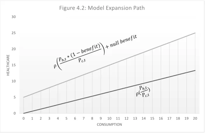
these enrollees pay a price of 0 for those services covered by Medicaid. States have a crucial effect on each person’s price of Medicaid because the state both determines the size of the subsidy given to citizens as well as which services are covered. Therefore each state has a great deal of impact on the healthcare decisions of their poorest citizens each year. It is further important to note that this subsidy for provided services is not a cash payment to citizens or a voucher program of some cash value. Instead, Medicaid is structured as a reimbursement system where the healthcare providers are transferred payments by the government. As such, Medicaid outlays can only be sent to the healthcare providers and individuals can only use this subsidy on healthcare goods. Below is a model expansion path for a generic individual before and after the subsidy.
In this model case, this individual has a generic demand for two units of healthcare for every three units of other consumable goods due to the relative prices of healthcare and
0 5 10 15 20 25 30
0 1 2 3 4 5 6 7 8 9 10 11 12 13 14 15 16 17 18 19 20
H
EA
LT
H
CA
R
E
CONSUMPTION
23
consumption goods. The figure highlights how, as its income expands, the individual consumes more of each good type in fixed proportions, here those proportions are the same and
independent of the subsidy. Here, the individual is a utility maximizer. The top line clearly shows that the individual immediately is able to and will purchase more healthcare when they have Medicaid. The design of the Medicaid program is such that individuals with zero income are allowed an allotment of healthcare goods such as doctor’s visits free of charge. Therefore, the individual enrolled on Medicaid can consume a nonzero amount of healthcare goods while having no income and no consumption goods. The services an enrolled individual receives here are set at five units as an example, but that benefit reflects a critical decision of the state. Further, the top line has a slope of one which highlights how enrolling in Medicaid alters the relative prices for the individual. Previously health was relatively more expensive, but Medicaid
enrollment lowers the price that the individual observes for healthcare goods and they therefore purchase more healthcare goods as a result of enrollment in Medicaid. The theory of this study is that the state’s government complexion causes significant differences in the state’s decisions which leads to a different benefit size and utilization. The changes to the benefit then impact the individual’s health as increased or decreased access to health services result in an increase or decrease in the health of that person. The decision of the state with respect to the benefits of Medicaid is one of the key aspects of state level decisions examined below.
24
maximizing their income, it is in the individual’s interest to refrain from maximizing their income as losing the subsidy results in a decrease in the healthcare goods that they can purchase and by the utility function, a decrease in their overall utility. Furthermore, this figure does not visually demostrate the impact that quotas may have on individuals. As referenced in the case study, some states cap the benefits that an individual may receive under Medicaid. If an
individual was in one of those states where the program’s benefits are limited, then their price of healthcare ceases to be augmented at the point where they have consumed the entirety of the Medicaid benefit. Visually, this would alter the slope of the top line in figure 4.2 to having the same slope as the line for the individual not enrolled in the Medicaid program.
The state faces a welfare calculation similar to a utility framework where the state’s goal is to maximize welfare. The state faces the following Lagrangian which consists of the state’s welfare function and a Lagrangian multiplier multiplied by the state’s budget constraint:
𝐿𝑎𝑔𝑟𝑎𝑛𝑔𝑖𝑎𝑛 𝑓𝑜𝑟 𝑊𝑠,𝑡 =
(𝑤𝑠,𝑡∗ 𝐿𝑠,𝑡∗ (1 − 𝜏𝑠,𝑡))𝛽1∗ 𝐸𝑠,𝑡1−𝛽1−𝛽2∗ 𝐻𝑠,𝑡𝛽2+ 𝜑 ∗ (𝑤𝑠,𝑡∗ 𝐿𝑠,𝑡∗ 𝜏𝑠,𝑡− 𝑆𝑠,𝑡− 𝑅𝑠,𝑡)
Where s and t are the subscripts for the state and time while 𝑤𝑠,𝑡 is the wage across the state for total labor hours 𝐿𝑠,𝑡 (the sum of all 𝑙𝑠,𝑡), 𝜏𝑠,𝑡 is the tax rate, 𝑆𝑠,𝑡 is the total Medicaid subsidy in the state which is equivalent to Medicaid spending, 𝐸𝑠,𝑡 is the employment seen by a state’s citizens, 𝐻𝑠,𝑡 is the healthcare coverage in the state, 𝜑 is a Lagrangian multiplier, and 𝑅𝑠,𝑡
represents the rest of the state’s spending that is not related to Medicaid. The exponents 𝛽1 and
𝛽2 are both constrained to values between zero and one with a sum of less than one. For the purposes of this paper, healthcare coverage 𝐻𝑠,𝑡 can be further refined to be a function of 𝑆𝑠,𝑡, the state’s total spending on Medicaid. The literature on Medicaid expansions indicates that
25
𝑤𝑠,𝑡∗ 𝐿𝑠,𝑡∗ 𝜏𝑠,𝑡
(3.1.1)
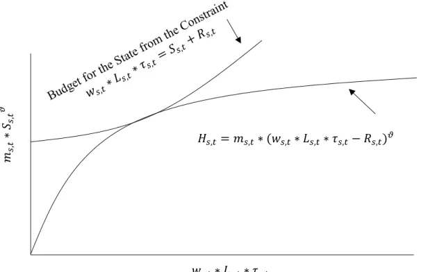
Figure 4.3.1: Example of Healthcare Coverage in a Given State
𝑚𝑠
,𝑡
∗
𝑆𝑠,𝑡
𝜗
𝐻𝑠,𝑡 = 𝑚𝑠,𝑡∗ (𝑤𝑠,𝑡∗ 𝐿𝑠,𝑡∗ 𝜏𝑠,𝑡− 𝑅𝑠,𝑡)𝜗
Medicaid coverage is a function of spending with decreasing marginal returns, therefore it will be modeled thusly:
𝐻𝑠,𝑡= 𝑚𝑠,𝑡∗ 𝑆𝑠,𝑡𝜗 with 𝑑𝐻
𝑑𝑆 > 0 and 𝑑2𝐻 𝑑𝑆2 ≤ 0
Where 𝜗 is greater than 0 but less than or equal to 1 and 𝑚𝑠,𝑡 is a constant. Equation 3.1.1 can be illustrated in the following figure:
26
state’s welfare maximizing point is seen where the 𝐻𝑠,𝑡 curve is tangent to the budget line. This assumes that the state is a welfare maximizer while attempting to minimize their expenditure level which is equivalent to the state minimizing the tax rate. The tangency of the two curves therefore reflects the optimal, welfare maximizing, value of 𝐻𝑠,𝑡. Furthermore, the subsidy can be recalibrated as a function of taxes. Each state devotes a certain amount of their tax revenue to their Medicaid program, the above theoretical model can be redefined in terms of this “Medicaid subsidy” which is equal to the percent of each dollar of personal income in the state that the state collect as tax to specifically pay for Medicaid. This is related by the following equations where
𝑠𝑠,𝑡 is the Medicaid subsidy.
𝑆𝑠,𝑡 = 𝑤𝑠,𝑡∗ 𝐿𝑠,𝑡∗ 𝑠𝑠,𝑡 and so (𝑤𝑠,𝑡∗ 𝐿𝑠,𝑡∗ 𝜏𝑠,𝑡− 𝑆𝑠,𝑡− 𝑅𝑠,𝑡) = (𝑤𝑠,𝑡∗ 𝐿𝑠,𝑡∗ (𝜏𝑠,𝑡− 𝑠𝑠,𝑡) − 𝑅𝑠,𝑡)
This means that the state’s welfare Lagrangian can be related as:
𝐿𝑎𝑔𝑟𝑎𝑛𝑔𝑖𝑎𝑛 𝑓𝑜𝑟 𝑊𝑠,𝑡 = (𝑤 ∗ 𝐿𝑠,𝑡∗ (1 − 𝜏𝑠,𝑡))
𝛽1
∗ 𝐸𝑠,𝑡1−𝛽1−𝛽2 ∗ (𝑚𝑠,𝑡∗ (𝑤𝑠,𝑡∗ 𝐿𝑠,𝑡∗ 𝑠𝑠,𝑡) 𝜗)𝛽2
+ 𝜑 ∗ (𝑤𝑠,𝑡∗ 𝐿𝑠,𝑡∗ (𝜏𝑠,𝑡− 𝑠𝑠,𝑡) − 𝑅𝑠,𝑡)
The aspects of this equation over which the state government can exercise control are the critical parts of this analysis presented in Section VII. The state government has control over 𝑠𝑠,𝑡 and 𝜏𝑠,𝑡 while being constrained by the revenue the state brings in 𝑊𝑠,𝑡∗ 𝐿𝑠,𝑡∗ 𝜏𝑠,𝑡 less the amount the state spends which for simplicity are viewed as spending on either Medicaid or on all other programs. When the state government maximizes its utility with respect to what it may control, the following are the first order conditions:
(3.1.2)
27
𝑑𝐿𝑎𝑔𝑟𝑎𝑛𝑔𝑖𝑎𝑛
𝑑𝜏𝑠,𝑡 = −𝑤𝑠,𝑡∗ 𝐿𝑠,𝑡∗ 𝛽1∗ (𝑤𝑠,𝑡∗ 𝐿𝑠,𝑡∗ (1 − 𝜏𝑠,𝑡))
𝛽1−1
∗ 𝐸𝑠,𝑡1−𝛽1−𝛽2
∗ (𝑚𝑠,𝑡∗ (𝑤𝑠,𝑡∗ 𝐿𝑠,𝑡∗ 𝑠𝑠,𝑡) 𝜗)𝛽2 + 𝜑 ∗ 𝑤𝑠,𝑡∗ 𝐿𝑠,𝑡 = 0
𝑑𝐿𝑎𝑔𝑟𝑎𝑛𝑔𝑖𝑎𝑛 𝑑𝑠𝑠,𝑡
= 𝜗 ∗ 𝛽2∗ 𝑚𝑠,𝑡∗ 𝑤𝑠,𝑡∗ 𝐿𝑠,𝑡∗ 𝐸𝑠,𝑡1−𝛽1−𝛽2 ∗ (𝑤𝑠,𝑡∗ 𝐿𝑠,𝑡∗ 𝑠𝑠,𝑡)𝜗−1
∗ (𝑚𝑠,𝑡∗ (𝑤𝑠,𝑡∗ 𝐿𝑠,𝑡∗ 𝑠𝑠,𝑡)𝜗)𝛽2−1∗ (𝑤𝑠,𝑡∗ 𝐿𝑠,𝑡∗ (1 − 𝜏𝑠,𝑡))𝛽1− 𝜑 ∗ 𝑤𝑠,𝑡∗ 𝐿𝑠,𝑡= 0
The states also face the following budget constraint:
𝑤𝑠,𝑡∗ 𝐿𝑠,𝑡∗ 𝜏𝑠,𝑡= 𝑤𝑠,𝑡∗ 𝐿𝑠,𝑡∗ 𝑠𝑠,𝑡+ 𝑅𝑠,𝑡
When solved for the equilibrium value of the Medicaid subsidy, the above equations yield the following equation:
𝑠𝑠,𝑡=
𝜗 ∗ 𝛽2∗ (1 − 𝜏𝑠,𝑡) 𝛽1
The state derives its welfare from three key factors: income, employment and healthcare coverage. The definition of the equation for healthcare coverage indicates that as 𝑠𝑠,𝑡 and income increase, so does 𝐻𝑠,𝑡. The state also sees an increase in healthcare spending when the Medicaid subsidy increases as well as when incomes increase. When looked at in relative isolation as seen in equation 4.2 in the appendix, the Medicaid subsidy decreases as the tax rate increases, the tax rate is not the sole driver of the Medicaid subsidy as the values of 𝜗, 𝛽1 and 𝛽2 each impact the Medicaid subsidy.
A key factor in both the theoretical and empirical model of this paper is the complexion of state governments. It is important to note that complexion does not directly appear in the state’s utility calculation. However, government complexion is important to the relationships
(3.5)
(3.6) (3.3)
28
Welfare for a given State with a Unified Government
Welfare for that same State under the same Conditions with a
Divided Government
above. Different state government complexions alter the composition of the Medicaid program in each state. Namely, the government complexion of the state alters the utility function by altering the corresponding 𝜗, 𝛽1 and 𝛽2 values within the utility function. The thesis presented earlier posits that a movement towards unified government, numerically defined as a positive increase in government complexion, results in a negative change in health outcomes which is represented as ℎ𝑡. This implies that a shift towards unified government complexion increases the tax rate, decreases healthcare spending and decreases healthcare coverage. These connections allow for the relationships including government complexion to be modeled since the above expression highlights the theorized relationship between government complexion and the rest of the model.
The following figure depicts how this relationship posited by the thesis comes to fruition in the welfare functions of the states:
Figure 4.3.2: Welfare Differences Caused by Government Complexion
𝑤𝑠
,𝑡
∗
𝐿𝑠,𝑡
∗
(1
−
𝜏𝑠,𝑡
)
29
As reflected in the thesis, when a state has a unified government, that state’s welfare function places a much larger point of emphasis on maximizing the citizen’s post tax income (the values on the y-axis). Divided governments pay much more heed to healthcare coverage (the values of the x-axis). In turn, healthcare coverage has a positive direct relationship with the health outcomes, completing the thesis. As in the previous figure, the state faces a budget constraint. This constraint has multiple key features, one of these is the fact that each state’s set of indifference curves run tangential to the budget curve when the state maximizes its welfare. Another key feature is the fact that the Medicaid subsidy 𝑠𝑠,𝑡 and the general tax rate 𝜏𝑠,𝑡 have an impact on each other. In the outline of the theoretical model this was expected. The outline highlights that general tax rate increases impact Medicaid spending, specifically that divided state governments increase taxes which increases Medicaid spending (which is seen in an increase in Medicaid subsidies). This relationship is accounted for in the calculation of the Medicaid subsidy seen in equation 3.6, but the relationship between the overall tax rate and Medicaid subsidies is also in the budget constraint of equation 3.5. The fact that these variables appear twice in the equations above adds complexity to the estimation of these relationships. This is more fully explored in the discussion on the empirical model and the results of the estimation.
30
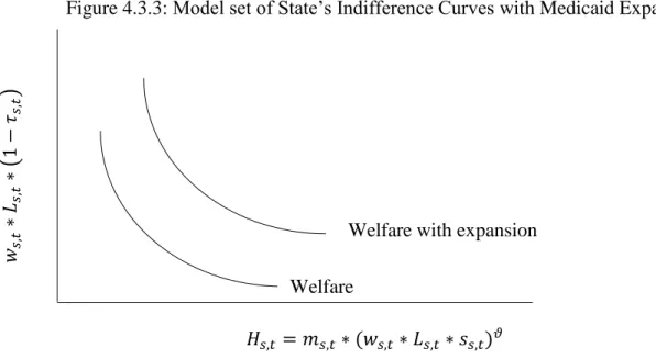
of the costs of the new enrollees while changes made in 2014 would be paid for by the federal government. The states also receive no reimbursement from the federal government for the additional administrative costs of enrolling more individuals nor for the costs associated with enticing the newly eligible to sign up for the program. As such, the states faced a key choice to make for the years at the end of the sample that is independent of their complexion for the rest of the period. This choice will be modeled in later iterations of the model to highlight the impact that the decisions states make have on their Medicaid programs. Below is a model indifference curve for a state who faces the choice to expand Medicaid:
This figure highlights the welfare balance a state attempts to maintain while employment is held constant. This figure is not one that all states would see or experience. In this sample case, the expansion designed by the Affordable Care Act, the states are presented with an opportunity to move to a higher indifference curve due to an influx of federal dollars to fund Medicaid expansions. However, this change is not entirely one way as the states still have an added cost to expanding the program which would need to be paid for by increasing Medicaid subsidies slightly. The states therefore face another choice, whether to expand Medicaid at a
Welfare with expansion Welfare
𝑤𝑠
,𝑡
∗
𝐿𝑠,𝑡
∗
(1
−
𝜏𝑠,𝑡
)
𝐻𝑠,𝑡= 𝑚𝑠,𝑡∗ (𝑤𝑠,𝑡∗ 𝐿𝑠,𝑡∗ 𝑠𝑠,𝑡)𝜗
31
greatly reduced cost or to stand pat throughout this time period and incur no additional program costs. In the figure above, the state would be able to move to a higher indifference curve but their move is not at a direct horizontal shift. The state will still have a tradeoff with the Medicaid expansion which will require an increase in taxes. This decision is why, under this framework, not all states choose to expand Medicaid. Some states will have a welfare function that favors low taxes much more than healthcare coverage. In other words, those states have 𝛽1values which are substantially larger than their 𝛽2 values. Therefore, it is possible for some states to face a net decrease in their welfare when given an opportunity to expand Medicaid. The theory of this study is that the states with welfare curves of this shape are the states with a unified government. Whether or not this decision is influenced in any way by partisan complexion in reality is
unclear, but this relationship is an interesting facet of this data which will be explored in forthcoming sections.
Figure 4.3.3 has further implications for the empirical model of the theoretical
relationships. The state’s welfare indifference curves underscore the fact that the state is acting as an economic agent making decisions within an established framework. The state faces a key tradeoff between maximizing their citizen’s incomes and maximizing their healthcare coverage. Most importantly, the state’s preferences which are motivated by government complexion determine the shape of and position on the state’s welfare indifference curve. Taken all together, the theoretical model clearly establishes the data necessary for the estimation of these
relationships.
V. Data Sources and Summary Statistics of Key Variables
32
their welfare status, income, healthcare coverage and health condition. The particular data used for this analysis will consist of Current Population Survey data from 1999-2014. The focus will be from 2000-2014, but some 1999 data is needed to determine the impact of lagged effects. This data is curated by the University of Minnesota Population Center’s Integrated Public Use
Microdata Series (IPUMS) center. The year 2000 reflects the best starting point for the data as Medicaid was significantly altered in the 1990s by the Clinton administration. As part of a larger welfare reform package, a large part of Medicaid’s funding and discretionary allocations was transferred to the states from the federal government. By the year 2000, these changes had fully taken place which precludes any of the administrative aspects of the transfer of the program to the states from introducing error into a model. The final year of the dataset being 2014
corresponds to the last year of complete data available from both the Current Population Survey and other ancillary data sources. These ancillary data sources correspond to the sources for the complexion of state government data, the information on state taxation and the information on state Medicaid expenditures. The complexion of state government data is widely available from a variety of sources that curate the information from the states themselves. The specific dataset used in this analysis of state government complexion is from the National Conference of State Legislatures which covers the entire time period in question. Despite the fact that that
organization is focused on state legislatures, the dataset also includes information on the
33
the state spending on Medicaid closely. Supplemental data on participation rates not found in the data from the Centers for Medicare and Medicaid Services will come from the Kaiser Family Foundation’s Commission on Medicaid and the Uninsured.
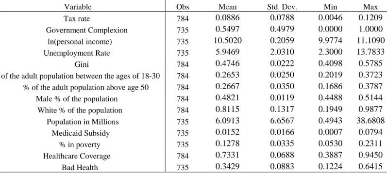
Each of the variables used in the estimation is shown in the table below. These variables either directly relate to the theoretical model or are components of the vector which controls for the characteristics of each state to increase the accuracy of the estimation. Below is a summary of the key variables:
Table 5.1: Summary Statistics of Key Variables
Variable Obs Mean Std. Dev. Min Max
Tax rate 784 0.0886 0.0788 0.0046 0.1209
Government Complexion 735 0.5497 0.4979 0.0000 1.0000
ln(personal income) 735 10.5020 0.2059 9.9774 11.1090
Unemployment Rate 735 5.9469 2.0310 2.3000 13.7833
Gini 784 0.4746 0.0222 0.4098 0.5785
% of the adult population between the ages of 18-30 784 0.2653 0.0250 0.2019 0.3723
% of the adult population above age 50 784 0.2667 0.0350 0.1686 0.3787
Male % of the population 784 0.4821 0.0119 0.4488 0.5144
White % of the population 784 0.8115 0.1317 0.1949 0.9877
Population in Millions 735 6.0913 6.6567 0.4943 38.6808
Medicaid Subsidy 735 0.0152 0.0166 0.0007 0.0794
% in poverty 735 0.1278 0.0335 0.0530 0.2311
Healthcare Coverage 784 0.7331 0.0688 0.3887 0.9450
Bad Health 735 0.3429 0.0883 0.1224 0.6415
Note: The above table contains simple summary statistics for all of the variables to be used in the regressions in the following sections.
34
35
tax revenue that the state extracts from each individual divided by average personal income in the state. The Medicaid subsidy is calculated in a similar fashion, as the total Medicaid spending per person in the state divided by average personal income. The Medicaid subsidy will be how this analysis will approach healthcare spending from the state on the Medicaid enrolled
population. When this is calibrated, federal Medicaid dollars are excluded from the analysis. For most of the timeframe this data examines, the share of all Medicaid funding from the federal government is consistent. In the last years of the sample, the share of all Medicaid dollars from the federal government decreases because, when states expanded Medicaid as part of the Affordable Care Act, the federal government bore a larger share of the cost than normal. To confront potential error source, estimations of the empirical models possess variables which control for the Medicaid expansion. These variables which control for the Medicaid expansion will be further explored in the results section when they are introduced. The Medicaid subsidy variable creates a subsidy size in every year which is proportional to the size of the Medicaid program in a state in a given year.
VI. Empirical Model
The empirical model will capture the relationship between each phase of the theoretical model. The first two equations highlighted below display the relationship between the
complexion of the state government and taxation and then the effect of each of those on revenue collection specifically for healthcare spending. Each of these equations will feature unique coefficients and unique error terms. Using the same variables as defined earlier in the discussion of the theoretical model:
𝜏𝑠,𝑡 = 𝛽1+ 𝛽2% 𝑏𝑒𝑙𝑜𝑤 𝑝𝑜𝑣𝑒𝑟𝑡𝑦 𝑙𝑖𝑛𝑒𝑠,𝑡+ 𝛽3𝐺𝐶𝑠,𝑡+ 𝜀1,𝑠,𝑡
𝑠𝑠,𝑡 = 𝛾1+ 𝛾2𝜏𝑠,𝑡+ 𝛾3% 𝑏𝑒𝑙𝑜𝑤 𝑝𝑜𝑣𝑒𝑟𝑡𝑦 𝑙𝑖𝑛𝑒𝑠,𝑡+ 𝛾4𝐺𝐶𝑠,𝑡 + 𝜀2,𝑠,𝑡 (6.1)
36
Each of these equations needs to account for external factors not inherently related to the theoretical model but captured in the welfare maximization for the state. Therefore each equation includes the percent of the population below the poverty line. This variable will proxy for how wealthy a state is. It is important that this variable is used here rather than personal income for mechanical reasons. The calculation of the tax rates in both equations is as a share of personal income in a state. If personal income were used as an independent variable in the estimation of variables constructed with personal income as factor then the estimation would yield biased coefficients. The first dependent variable is the tax rate. The overall tax variable, 𝜏𝑠,𝑡, refers to the tax rate on each marginal dollar earned in the state calculated in the first equation. It is designed to capture the size of the tax burden that each state puts on its citizens. This factor is related to personal income as richer states can levy a lower tax rate and still reap substantial revenues. The final variable in equation 6.1, 𝐺𝐶𝑠,𝑡, is the government complexion at time t in each state. In the second equation, the independent variable is the Medicaid subsidy, a reflection of how much that only the state spends on Medicaid. If this relationship is estimated in a simple OLS-style framework, then the second equation in this form has a large amount of bias. This bias originates from the fact that the overall tax rate and the Medicaid subsidy are tied together by the state’s budget constraint. In future estimations outside of an OLS-type framework, this direct relationship will be explored but in the initial estimation of the second equation, the general tax rate variable will be omitted. From there, the next two equations will look at the effect of the Medicaid subsidy on coverage and then the combination of those two upon healthcare outcomes.
𝐻𝑠,𝑡= 𝜌1+ 𝜌2𝐺𝐶𝑠,𝑡+ 𝜌3𝐻𝑠,𝑡−1+ 𝜌4ℎ𝑠,𝑡−1+ 𝜀3,𝑠,𝑡
ℎ𝑠,𝑡 = 𝜔1+ 𝜔2𝑠𝑠,𝑡+ 𝜔3ℎ𝑠,𝑡−1+ 𝜔4𝐻𝑠,𝑡+ 𝜔5𝑝𝑒𝑟𝑠𝑜𝑛𝑎𝑙 𝑖𝑛𝑐𝑜𝑚𝑒𝑠,𝑡+ 𝜀4,𝑠,𝑡 (6.3)
37
Health coverage (variable 𝐻𝑠,𝑡) is the percent of all enrolled citizens in Medicaid compared to the number of people eligible in that state at that time. This essentially becomes the Medicaid participation rate. The third equation features a lag of that same variable, the same government complexion factor seen in the other equations and a lagged physical health factor. The final equation determines health outcomes of those enrolled in Medicaid. This projects health (variable ℎ𝑠,𝑡) as a function of the Medicaid subsidy, lagged health and health coverage and income in the current time. The lagged variables are included here in equations 6.3 and 6.4 because these factors are clearly influenced by the value they had in the prior period. For equation 6.3, healthcare coverage in the current year is impacted by the share of eligible people who had coverage last year, these citizens would roll over their program benefits from one year to the next. Healthcare coverage is also impacted by how sick the state was in the previous period since, if the state is sicker, those eligible for powerful healthcare subsidies are more likely to enroll in Medicaid and drive up future enrollments. In equation 6.4 the variable for health outcomes has a one year-lag because health in the current time period is highly correlated with health in the previous time period. This study makes several assumptions about the lagged variables. If someone is currently sick, there is an increased likelihood that they were sick in the past and will be in the future, therefore the one year lag must be included. These lagged variables are only a one year lag as opposed to a multiyear lag since the changes to healthcare coverage are believed to appear quickly in the data. Further, for the lagged variables in each equation, the variable’s value in the previous year contains all of the information contained in all the other prior periods’ data as well. Therefore the previous year is the only necessary lag.
38
optimal model, the equations for taxation revenue, healthcare spending and health should be simultaneously solved as a system of equations rather than solved for independently. When estimated simultaneously, these equations will be estimated in a two stage least squares process. This process is selected rather than three stage least squares as two stage least squares is more robust in this situation due to the fact that it is less sensitive to the precision of the model’s calibration. 11 Another important factor to account for when solving these equations is to ensure that they are grouped into their proper state and time subscripted groups. This will be done by controlling for the fixed state and year effects when conducting the estimations.
Beyond simple econometric controls for fixed state and year effects, the background
conditions of each state deserve consideration in the estimation of these models. Therefore there are two key vectors added to the models in some iterations of the estimation of these equations. The model needs to control for the background demographic conditions in each state. To make this possible the estimations will feature a controls vector containing information about the state in that given time. The second key vector added for some estimations is whether or not the state chose to expand Medicaid as part of the Affordable Care Act.
VII. Results, Modelling and Discussion
Due to the nature of the empirical models, four iterations of the estimations of the models are produced. The first iteration of the model is a simple iteration where each of the equations is estimated separately with none of the control factors present and no time lags in the model outside of what was detailed in the empirical model. The estimation technique for the first iteration is a cross-sectional time-series FGLS regression with generalized least squares
39
coefficients and heteroskedastic panels. Further, the estimation controls for both state and year fixed effects. The first iteration of the first equation is as presented in the empirical model section and is as follows:
𝜏𝑠,𝑡 = 𝛽1+ 𝛽2% 𝑏𝑒𝑙𝑜𝑤 𝑝𝑜𝑣𝑒𝑟𝑡𝑦 𝑙𝑖𝑛𝑒𝑠,𝑡+ 𝛽3𝐺𝐶𝑠,𝑡+ 𝜀1,𝑠,𝑡
The results of this equation are in table 7.1.1 in the appendix. The results of the first regression support the theoretical model. Government complexion has a positive and statistically significant impact on the tax rate. The coefficient on government complexion is 0.0065 which means that unified governments increase the tax rate by 0.65 percentage point in the aggregate. This coefficient has a statistically significant z score of 3.94 which affirms the impact of state government complexion on tax rates in this estimation of the model. The theoretical model in section four posited that this would be the relationship observed and that it would have this sign. This equation also displays the expected relationship between percent in poverty and taxation. The percent of a state’s citizens in poverty has a statistically significant coefficient of 0.2171 with a z score of 4.93. The implication of this, that for each one percentage point increase in the share of a state’s population in poverty there is a 0.22 percentage point increase in the tax rate, is also aligned with the theoretical model. The theoretical model stated that if a state were
wealthier, here shown as an increase in personal income, then the state would experience a lower tax rate. This is because a rich state can sustain the same programs as a poor one with a lower tax rate due to the larger income present in the state.
The first iteration of the second equation is as follows:
𝑠𝑠,𝑡= 𝛾1+ 𝛾2% 𝑏𝑒𝑙𝑜𝑤 𝑝𝑜𝑣𝑒𝑟𝑡𝑦 𝑙𝑖𝑛𝑒𝑠,𝑡+ 𝛾3𝐺𝐶𝑠,𝑡+ 𝜀2,𝑠,𝑡 (7.1.2)
40
The results of this equation are in table 7.1.2 in the appendix. This equation produces statistically significant results for both government complexion and the percent of a state’s residents in poverty. This result is a refutation of a key part of the theoretical model. The
theoretical model posited that there was an inverse relationship between government complexion and the Medicaid subsidy. This estimation suggests the opposite is true. The government
complexion variable has a statistically significant positive coefficient of 0.0011 with a z score of 2.34. This effect implies that a shift in the state’s government complexion to unified from
divided results in a 0.11 percentage point increase in the Medicaid subsidy. This is a breakdown of the theoretical model in that the theoretical model posited the opposite relationship between the two. This result instead states that unified governments have a positive effect on the Medicaid subsidy. It was expected that the coefficient on government complexion would be negative and that it would be large as it was posited that the effect on spending was substantial. The poverty rate in the state also has a statistically significant relationship with a z score of 3.19 and a coefficient of 0.0416. This result states that as the poverty rate increases by one percentage point, the state’s Medicaid subsidy increases by 0.0416 percentage points. This result is expected to be significant because an impoverished population should increase a state’s healthcare
spending. Since Medicaid is a program for low income Americans, as the poverty in a state increases, the spending on Medicaid should increase. The materialization of that finding here lends credence to the theoretical model as it comports with the intuition of the study.
The largest sources of variation in Medicaid subsidy are the state effects and the year effects. These are contained in table 7.1.2.1. In all of the analysis of state effects contained in this section, the state effects view Alabama as the base case due to the fact that it is first in the
41
results imply that on aggregate Kentucky has the highest Medicaid subsidy after controlling for government complexion and the percent of residents in poverty while Tennessee has the
smallest. The state of Kentucky provided a Medicaid subsidy 2.07 percentage points above the base case on all income in the state for allocations on Medicaid, the largest such extra levy in the nation. By contrast, Tennessee has a subsidy 2.08 percentage points lower than the base case on aggregate for their Medicaid funding. North Carolina has a 0.23 percentage point subsidy
reduction compared to the base case. The z score of the North Carolina state effect is -0.31 which implies that it is not possible to affirm the existence of this relative reduction at a reasonable level of statistical confidence. California, another state considered in the overview of state Medicaid programs, has a 1.34 percentage point subsidy cut relative to the base case.
California’s state effect has a z score of -1.91 which is not significant at the 95% confidence level but it is significant at the 90% confidence level.
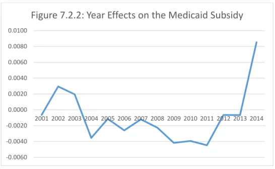
To illustrate the growth of the Medicaid program over time, the year effects are graphed below:
-0.0040 -0.0020 0.0000 0.0020 0.0040 0.0060 0.0080 0.0100 0.0120
42
The year effect is statistically significant in nine of the years in the record. Most notably, the year effect is larger at the start and the close of the sample. The Medicaid subsidy decreases to a relatively stable rate below the base case of the year 2000 from 2004 to 2011. The recession clearly negatively impacts Medicaid subsidies for a four year period as there are statistically significant negative year effects for 2008-2011. However, spending on Medicaid resumes increasing from 2011 to 2012 and continues to increase until 2014. The coefficients on the year effects are large, especially when compared with the coefficients on the variables. This rapid increase, and largest year effect, coincides with the passage of the Affordable Care Act. Further, as part of that law, the Medicaid expansion in many states fully opened in 2014 which appears to have impacted the Medicaid subsidy as this year has the largest increase of any year, resulting in a 0.96 percentage point increase in the Medicaid subsidy in the aggregate. This suggests that the state’s decision to expand Medicaid is crucially important to the Medicaid subsidy. This supports the theoretical model by showcasing the importance of the policy decisions that states make with respect to healthcare policy. It is important that the Medicaid subsidy still only addresses the state’s allocations to Medicaid. The size of the state’s Medicaid subsidy is significantly impacted by the decision to expand Medicaid even though much of the funds for the expansion comes from the federal government. This result also underscores a key precept of the theoretical model, that the decisions that states make matter and have an impact on their citizens.
The initial iteration of equation three is as follows:
𝐻𝑠,𝑡= 𝜌1+ 𝜌2𝐺𝐶𝑠,𝑡+ 𝜌3𝐻𝑠,𝑡−1+ 𝜌4ℎ𝑠,𝑡−1+ 𝜀3,𝑠,𝑡
The results of this estimation are seen in table 7.1.3. The theoretical model is supported by the results of this estimation. The theoretical model hypothesized that unified government would decrease Medicaid coverage in a state. That result is borne out by this estimation as the