Part II:
Sequential Problems
Up to this point, we have assumed that we make a single decision at one point in time, but many important problems require that we make a series of decisions. The same principle of maximum expected utility still applies, but optimal decision making in a sequential context requires reasoning about future sequences of actions and observations. This part of the book will discuss sequential decision problems in stochastic environments. We will focus on a general formulation of sequential decision problems under the assumption that the model is known and that the environment is fully observable. We will relax both of these assumptions later. Our discussion will begin with the introduction of theMarkov decision process, the standard mathematical model for sequential decision problems. We will discuss several approaches for inding exact solutions. Because large problems sometimes do not permit exact solutions to be eiciently found, we will discuss a collection of both oline and online approximate solution methods along with a type of method that involves directly searching the space of parameterized decision policies. Finally, we will discuss approaches for validating that our decision strategies will perform as expected when deployed in the real world.
7 Exact Solution Methods
This chapter introduces a model known as a Markov decision process to represent sequential decision problems where the efects of our actions are uncertain.1
1Such models were originally stud-ied in the 1950s. R. E. Bellman, Dy-namic Programming. Princeton Uni-versity Press, 1957. A modern treat-ment can be found in M. L. Put-erman,Markov Decision Processes: Discrete Stochastic Dynamic Program-ming. Wiley, 2005.
We begin with a description of the model, which speciies both the stochastic dynamics of the system as well as the utility associated with its evolution. Diferent algorithms can be used to compute the utility associated with a decision strategy and to search for an optimal strategy. Under certain assumptions, we can ind exact solutions to Markov decision processes. Later chapters will discuss approximation methods that tend to scale better to larger problems.
7.1 Markov Decision Processes
In aMarkov decision process(MDP), we choose actionatat timetbased on
observ-ing statest. We then receive a rewardrt. Theaction spaceAis the set of possible
actions, and thestate spaceSis the set of possible states. Some of the algorithms assume these sets are inite, but this is not required in general. The state evolves probabilistically based on the current state and action we take. The assumption that the next state depends only on the current state and action and not on any prior state or action is known as theMarkov assumption.
A1 A2 A3
R1 R2 R3
S1 S2 S3
Figure 7.1. Markov decision pro-cess decision diagram.
At
Rt
St St+1 Figure 7.2. Stationary Markov de-cision process dede-cision diagram. An MDP can be represented using a decision network as shown in igure 7.1.
There are information edges (not shown in the igure) fromA1:t−1andS1:ttoAt.
The utility function is decomposed into rewardsR1:t. We focus onstationaryMDPs
in whichP(St+1 | St,At)andP(Rt | St,At)do not vary with time. Stationary
MDPs can be compactly represented by a dynamic decision diagram as shown in igure 7.2. Thestate transition modelT(s′ | s,a)represents the probability of transitioning from statestos′after executing actiona. Thereward functionR(s,a) represents the expected reward received when executing actionafrom states.
The reward function is a deterministic function ofsandabecause it represents an expectation, but rewards may be generated stochastically in the environment or even depend upon the resulting next state.2Example 7.1 shows how to frame
2For example, if the reward de-pends on the next state as given byR(s,a,s′), then the (expected)
reward function would be
R(s,a) =
∑
s′T(s′|s,a)R(s,a,s′)
a collision avoidance problem as an MDP.
The problem of aircraft collision avoidance can be formulated as an MDP. The states represent the positions and velocities of our aircraft and the intruder aircraft, and the actions represent whether we climb, descend, or stay level. We receive a large negative reward for colliding with the other aircraft and a small negative reward for climbing or descending.
Given knowledge of the current state, we must decide whether an avoid-ance maneuver is required. The problem is challenging because the positions of the aircraft evolve probabilistically and we want to make sure that we start our maneuver early enough to avoid collision but late enough so that we avoid unnecessary maneuvering.
Example 7.1. Aircraft collision avoidance framed as an MDP. struct MDP γ # discount factor � # state space � # action space T # transition function R # reward function
TR # sample transition and reward end
Algorithm 7.1. Data structure for an MDP. We will use theTRield later to sample the next state and reward given the current state and action:s′, r = TR(s, a).
The rewards in an MDP are treated as components in an additively decomposed utility function. In ainite horizonproblem withndecisions, the utility associated with a sequence of rewardsr1:nis simply
n
∑
t=1
rt (7.1)
The sum of rewards is sometimes called thereturn.
In anininite horizonproblem in which the number of decisions is unbounded, the sum of rewards can become ininite.3There are several ways to deine utility
3Suppose strategyAresults in a reward of1per time step and strat-egyBresults in a reward of100 per time step. Intuitively, a ratio-nal agent should prefer strategyB
over strategyA, but both provide
the same ininite expected utility. in terms of individual rewards in ininite horizon problems. One way is to impose
7.1. markov decision processes 129 adiscount factorγbetween0and1. The utility is given by
∞
∑
t=1
γt−1rt (7.2)
This value is sometimes called thediscounted return. So long as0≤γ<1and the rewards are inite, the utility will be inite. The discount factor makes it so that rewards in the present are worth more than rewards in the future, a concept that also appears in economics.
Another way to deine utility in ininite horizon problems is to use theaverage rewardgiven by lim n→∞ 1 n n
∑
t=1 rt (7.3)Thisaverage returnformulation can be attractive because we do not have to choose a discount factor, but there is often not a practical diference between this for-mulation and discounted return with a discount factor close to1. Because the
discounted return is often computationally simpler to work with, we will focus on the discounted formulation.
Apolicytells us what action to select given the past history of states and actions. The action to select at timet, given thehistoryht= (s1:t,a1:t−1), is writtenπt(ht).
Because the future states and rewards depend only on the current state and action (as made apparent in the conditional independence assumptions in igure 7.1), we can restrict our attention to policies that depend only on the current state.
In ininite horizon problems with stationary transitions and rewards, we can further restrict our attention tostationary policies, which do not depend on time. We will write the action associated with stationary policyπin statesasπ(s), without the temporal subscript. In inite horizon problems, however, it may be beneicial to select a diferent action depending on how many time steps are remaining. For example, when playing basketball, it is generally not a good strategy to attempt a half-court shot unless there are only a couple seconds remaining in the game.
The expected utility of executingπfrom statesis denotedUπ(s). In the context
of MDPs,Uπis often referred to as thevalue function. Anoptimal policyπ∗is a
policy that maximizes expected utility:4 4Doing so is consistent with the
maximum expected utility princi-ple introduced in section 6.4. π∗(s) =arg max
π
for all statess. Depending on the model, there may be multiple policies that are optimal. The value function associated with an optimal policyπ∗is called the
optimal value functionand is denotedU∗.
An optimal policy can be found by using a computational technique called dynamic programming,5 which involves simplifying a complicated problem by
5The term dynamic programming was coined by the American math-ematician R. Bellman (1920–1984). Dynamic refers to the fact that the problem is time-varying and pro-gramming refers to a methodology to ind an optimal program or deci-sion strategy. R. Bellman,Eye of the Hurricane: an Autobiography. World Scientiic, 1984.
breaking it down into simpler sub-problems in a recursive manner. Although we will focus on dynamic programming algorithms for MDPs, dynamic pro-gramming is a general technique that can be applied to a wide variety of other problems. For example, dynamic programming can be used in computing a Fi-bonacci sequence and inding the longest common subsequence between two
strings.6In general, algorithms that use dynamic programming for solving MDPs 6T. H. Cormen, C. E. Leiserson, R. L. Rivest, and C. Stein, Intro-duction to Algorithms, 3rd ed. MIT Press, 2009.
are much more eicient than brute force methods.
7.2 Policy Evaluation
Before we discuss how to go about computing an optimal policy, we will irst dis-cusspolicy evaluation, where we compute the value functionUπ. Policy evaluation
can be done iteratively. If the policy is executed for a single time step, the utility isUπ
1(s) =R(s,π(s)). Further steps can be obtained by applying thelookahead equation:
Uπk+1(s) =R(s,π(s)) +γ
∑
s′
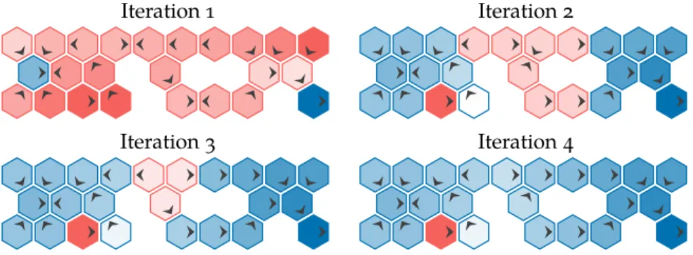
T(s′ |s,π(s))Ukπ(s′) (7.5) This equation is implemented in algorithm 7.2. Iterative policy evaluation is implemented in algorithm 7.3. Several iterations are shown in igure 7.3.
function lookahead(�::MDP, U, s, a)
�, T, R, γ = �.�, �.T, �.R, �.γ
return R(s,a) + γ*sum(T(s,a,s′)*U(s′) for s′ in �)
end
function lookahead(�::MDP, U::Vector, s, a)
�, T, R, γ = �.�, �.T, �.R, �.γ
return R(s,a) + γ*sum(T(s,a,s′)*U[i] for (i,s′) in enumerate(�))
end
Algorithm 7.2. Functions for com-puting the lookahead state-action value from a statesgiven an action ausing an estimate of the value functionUfor the MDP�. The sec-ond version handles the case when Uis a vector.
The value functionUπcan be computed to arbitrary precision given suicient
iterations. For an ininite horizon, we have Uπ(s) =R(s,π(s)) +γ
∑
s′
7.2. policy evaluation 131
function iterative_policy_evaluation(�::MDP, π, k_max)
�, T, R, γ = �.�, �.T, �.R, �.γ U = [0.0 for s in �] for k in 1:k_max U = [lookahead(�, U, s, π(s)) for s in �] end return U end
Algorithm 7.3. Iterative policy evaluation, which iteratively com-putes the value function for a pol-icyπfor MDP�with discrete state and action spaces usingk_max iter-ations.
Iteration 1 Iteration 2
Iteration 3 Iteration 4
−10 −8 −6 −4 −2 0 2 4 6 8 10
Figure 7.3. Iterative policy eval-uation used to evaluate an east-moving policy on the hex world problem (appendix F.1). The ar-rows indicate the direction recom-mended by the policy (i.e., always move east), and the colors indi-cate the values associated with the states. The values change with each iteration.
at convergence. Convergence can be proven using the fact that the update in
equation (7.5) is acontraction mapping(reviewed in appendix A.15).7 7See exercise 7.11. Policy evaluation can be done without iteration by solving a system of equations
in matrix form:
Uπ=Rπ+γTπUπ (7.7)
whereUπ andRπ are the utility and reward functions represented in vector form with|S| components. The|S| × |S|matrix Tπ contains state transition probabilities whereTπ
ij is the probability of transitioning from theith state to the jth state.
The value function is obtained as follows:
Uπ−γTπUπ=Rπ (7.8)
(I−γTπ)Uπ=Rπ (7.9)
Uπ= (I−γTπ)−1Rπ (7.10)
This method is implemented in algorithm 7.4. Solving forUπ in this way requiresO(|S|3)time. The method is used to evaluate a policy in igure 7.4.
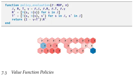
function policy_evaluation(�::MDP, π) �, R, T, γ = �.�, �.R, �.T, �.γ R′ = [R(s, π(s)) for s in �] T′ = [T(s, π(s), s′) for s in �, s′ in �] return (I - γ*T′)\R′ end
Algorithm 7.4. Exact policy eval-uation, which computes the value function for a policyπfor an MDP � with discrete state and action spaces.
Figure 7.4. Exact policy evaluation used to evaluate an east-moving policy for the hex world problem. The exact solution contains lower values than what was contained in the irst few steps of iterative pol-icy evaluation in igure 7.3. If we ran iterative policy evaluation for more iterations, it would converge to the same value function.
7.3 Value Function Policies
The previous section showed how to compute a value function associated with a policy. This section shows how to extract a policy from a value function, which we later use when generating optimal policies. Given a value functionU, which
7.3. value function policies 133 may or may not correspond to the optimal value function, we can construct a
policyπthat maximizes the lookahead equation introduced in equation (7.5): π(s) =arg max a R(s,a) +γ
∑
s′ T(s′ |s,a)U(s′) ! (7.11) We refer to this policy as agreedy policywith respect toU. IfUis the optimal value function, then the extracted policy is optimal. Algorithm 7.5 implements this idea.An alternative way to represent a policy is to use theaction value function, sometimes called theQ-function. The action value function represents the expected return when starting in states, taking actiona, and then continuing with the greedy policy with respect toQ:
Q(s,a) =R(s,a) +γ
∑
s′
T(s′ |s,a)U(s′) (7.12) From this action value function, we can obtain the value function,
U(s) =max
a Q(s,a) (7.13)
as well as the policy,
π(s) =arg max
a
Q(s,a) (7.14)
StoringQexplicitly for discrete problems requiresO(|S| × |A|)storage instead ofO(|S|)storage forU, but we do not have to useRandTto extract the policy. Policies can also be represented using theadvantage function, which quantiies the advantage of taking an action in comparison to the greedy action. It is deined in terms of the diference betweenQandU:
A(s,a) =Q(s,a)−U(s) (7.15) Greedy actions have zero advantage, and non-greedy actions have negative advan-tage. Some algorithms that we will discuss later in the book useUrepresentations, but others will useQorA.
struct ValueFunctionPolicy � # problem U # utility function end function greedy(�::MDP, U, s) u, a = _findmax(a->lookahead(�, U, s, a), �.�) return (a=a, u=u) end function (π::ValueFunctionPolicy)(s) return greedy(π.�, π.U, s).a end
Algorithm 7.5. A value function policy extracted from a value func-tionUfor an MDP�. Thegreedy function will be used in other algo-rithms.
7.4 Policy Iteration
Policy iteration(algorithm 7.6) is one way to compute an optimal policy. It in-volves iterating between policy evaluation (section 7.2) and policy improvement through lookahead (algorithm 7.5). Policy iteration is guaranteed to converge given any initial policy. It converges because there are initely many policies and every iteration improves the policy if it is possible to be improved. Figure 7.5 demonstrates policy iteration on the hex world problem.
struct PolicyIteration π # initial policy
k_max # maximum number of iterations end
function solve(M::PolicyIteration, �::MDP)
π, � = M.π, �.� converged = false for k = 1:M.k_max U = policy_evaluation(�, π) π′ = ValueFunctionPolicy(�, U) if all(π(s) == π′(s) for s in �) break end π = π′ end return π end
Algorithm 7.6. Policy iteration, which iteratively improves an ini-tial policyπto obtain an optimal policy for an MDP�with discrete state and action spaces.
7.5. value iteration 135
Iteration 1 Iteration 2
Iteration 3 Iteration 4
Figure 7.5. Policy iteration used to iteratively improve an initially east-moving policy on the hex world problem to obtain an optimal pol-icy. In the irst iteration, we see the value function associated with the east-moving policy and the arrows indicating the policy that is greedy with respect to that value function. Policy iteration converges in four iterations; if we ran for a ifth itera-tion, we would get the same policy. Policy iteration tends to be expensive because we must evaluate the policy in
each iteration. A variation of policy iteration is calledmodiied policy iteration,8 8M. L. Puterman and M. C. Shin, ‘‘Modiied Policy Iteration Algo-rithms for Discounted Markov De-cision Problems,’’Management Sci-ence, vol. 24, no. 11, pp. 1127–1137, 1978.
which approximates the value function using iterative policy evaluation instead of exact policy evaluation. A parameter in the modiied policy iteration algorithm is the number of policy evaluation iterations to perform between steps of policy improvement. If this parameter is1, then this approach is identical to value
iteration.
7.5 Value Iteration
Value iterationis an alternative to policy iteration that is often used because of its simplicity. Unlike policy improvement, value iteration updates the value function directly. It begins with any bounded value functionU, meaning that|U(s)|<∞ for alls. One common initialization isU(s) =0for alls.
The value function can be improved by applying theBellman equation:9 9Named for one of the pioneers of the ield of dynamic programming. R. E. Bellman, Dynamic Program-ming. Princeton University Press, 1957. Uk+1(s) =maxa R(s,a) +γ
∑
s′ T(s′ |s,a)Uk(s′) ! (7.16) This backup procedure is implemented in algorithm 7.7.function backup(�::MDP, U, s)
return maximum(lookahead(�, U, s, a) for a in �.�)
end
Algorithm 7.7. The backup proce-dure applied to an MDP�, which improves a value functionUat state s.
Repeated application of this update is guaranteed to converge on an optimal policy. Like iterative policy evaluation, we can use the fact that the update is a
contraction mapping to prove convergence.10This optimal policy is guaranteed 10See exercise 7.12. to satisfy: U∗(s) =max a R(s,a) +γ
∑
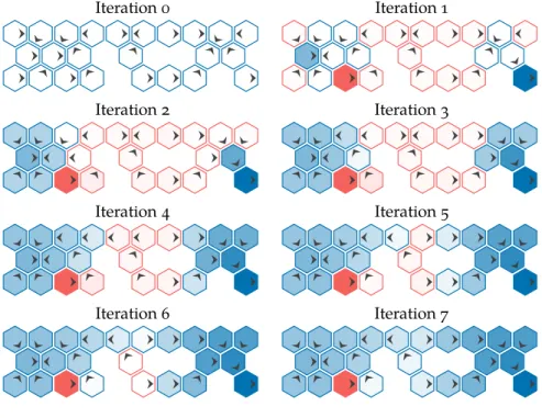
s′ T(s′|s,a)U∗(s′) ! (7.17) Further applications of Bellman’s equation once this equality holds do not change the policy. An optimal policy can be extracted fromU∗using equation (7.11). Value iteration is implemented in algorithm 7.8 and is applied to the hex world problem in igure 7.6.The implementation in algorithm 7.8 stops after a ixed number of iterations, but it is also common to terminate the iterations early based on the maximum change in value called theBellman residual,kUk+1−Ukk∞. If the Bellman residual
drops below some thresholdδ, then the iterations terminate. A Bellman residual ofδguarantees that the optimal value function obtained by value iteration is
withinǫ=δγ/(1−γ)ofU∗.11Discount factors closer to1signiicantly inlate 11See exercise 7.8. this error, leading to slower convergence. If we heavily discount future reward (γ
closer to0), then we do not need to iterate as much into the future. This efect is
demonstrated in example 7.2.
Knowing the maximum deviation of the estimated value function from the optimal value function,kUk−U∗k∞ < ǫ, allows us to bound the maximum deviation of reward obtained under the extracted policyπfrom an optimal policy π∗, thepolicy losskUπ−U∗k
∞. The policy loss is bounded by2ǫ.12 12To see why, see exercise 7.9.
struct ValueIteration
k_max # maximum number of iterations end
function solve(M::ValueIteration, �::MDP)
U = [0.0 for s in �.�] for k = 1:M.k_max U = [backup(�, U, s) for s in �.�] end return ValueFunctionPolicy(�, U) end
Algorithm 7.8. Value iteration, which iteratively improves a value functionUto obtain an optimal pol-icy for an MDP�with discrete state and action spaces. The method ter-minates afterk_maxiterations.
7.5. value iteration 137
Iteration 0 Iteration 1
Iteration 2 Iteration 3
Iteration 4 Iteration 5
Iteration 6 Iteration 7
Figure 7.6. Value iteration on the hex world problem to obtain an op-timal policy. Each hex is colored ac-cording to the value function and arrows indicate the policy that is greedy with respect to that value function.
Consider a simple variation of the hex world problem consisting of a straight line of tiles with a single consuming tile at the end producing10reward. The
discount factor directly afects the rate at which reward from the consuming tile propagates down the line to the other tiles, and thus how quickly value iteration converges.
γ=0.9 γ=0.5
Example 7.2. An example showing the efect of the discount factor on convergence of value iteration. In each case value iteration was run until the Bellman residual was less than1.
7.6. asynchronous value iteration 139
7.6 Asynchronous Value Iteration
Value iteration tends to be computationally intensive, as every entry in the value functionUkis updated in each iteration to obtainUk+1. Inasynchronous value itera-tion, only a subset of the states are updated in each iteration. Asynchronous value iteration is still guaranteed to converge on the optimal value function provided that each state is updated ininitely often.
One common asynchronous value iteration method,Gauss-Seidel value iteration (algorithm 7.9), sweeps through an ordering of the states and applies the Bellman update in place: U(s)←max a R(s,a) +γ
∑
s′ T(s′ |s,a)U(s′) ! (7.18) The computational savings lies in not having to construct a second value function in memory in each iteration. Gauss-Seidel value iteration can converge morequickly than standard value iteration depending on the ordering chosen.13In 13A poor ordering in Gauss-Seidel value iteration cannot cause the al-gorithm to be slower than standard value iteration.
some problems, the state contains a time index that increments deterministically forward in time. If we apply Gauss-Seidel value iteration starting at the last time index and work our way backwards, this process is sometimes calledbackwards induction value iteration. An example of the impact of the state ordering is given in example 7.3.
struct GaussSeidelValueIteration
k_max # maximum number of iterations end
function solve(M::GaussSeidelValueIteration, �::MDP)
�, �, T, R, γ = �.�, �.�, �.T, �.R, �.γ U = [0.0 for s in �] for k = 1:M.k_max for (s, i) in enumerate(�) u = backup(�, U, s) U[i] = u end end return ValueFunctionPolicy(�, U) end Algorithm 7.9. Asynchronous value iteration, which updates states in a diferent manner to value iteration, often saving com-putation time. The method termi-nates afterk_maxiterations.
Consider the linear variation of the hex world problem from example 7.2. We can solve the same problem using asynchronous value iteration. The ordering of the states directly afects the rate at which reward from the consuming tile propagates down the line to the other tiles, and thus how quickly the method converges.
Left to Right Right to Left
Example 7.3. An example show-ing the efect of the state ordershow-ing on convergence of asynchronous value iteration. In this case, evalu-ating right to left allows for conver-gence in far fewer iterations.
7.7. linear program formulation 141
7.7 Linear Program Formulation
The problem of inding an optimal policy can be formulated as alinear program, which is an optimization problem with a linear objective function and a set of linear equality or inequality constraints. Once a problem is represented as a linear
program, we can use one of many diferent linear programming solvers.14 14For an overview of linear pro-gramming, see R. Vanderbei, Lin-ear Programming, Foundations and Extensions, 4th ed. Springer, 2014. To show how we can convert the Bellman equation into a linear program, we
begin by replacing the equality in the Bellman equation with a set of inequality
constraints while minimizingU(s)at each states:15 15Intuitively, we want to push the valueU(s)at all statessdown to
convert the inequality constraints into equality constraints. Hence, we minimize the sum of all utili-ties. minimize
∑
s U(s) subject toU(s)≥max a R(s,a) +γ∑
s′ T(s′|s,a)U(s′) ! for alls (7.19) The variables in the optimization are the utilities at each state. Once we know those utilities, we can extract an optimal policy using equation (7.11).The maximization in the inequality constraints can be replaced by a set of linear constraints, making it a linear program:
minimize
∑
s U(s)
subject toU(s)≥R(s,a) +γ
∑
s′
T(s′|s,a)U(s′)for allsanda (7.20) In the linear program above, the number of variables is equal to the number of states and the number of constraints is equal to the number of states times the number of actions. Because linear programs can be solved in polynomial time,16MDPs can be solved in polynomial time. Although a linear
program-16This was proven by L. G. Khachiyan, ‘‘Polynomial Algo-rithms in Linear Programming,’’
USSR Computational Mathematics and Mathematical Physics, vol. 20, no. 1, pp. 53–72, 1980. Modern algorithms tend to be more eicient in practice.
ming approach provides this asymptotic complexity guarantee, it is often more eicient in practice to simply use value iteration. Algorithm 7.10 provides an implementation.
7.8 Linear Systems with Quadratic Reward
So far, we have assumed discrete state and action spaces. This section relaxes this assumption, allowing for continuous, vector-valued states and actions. The Bellman equation for discrete problems can be modiied as follows:17
17This section assumes the prob-lem is undiscounted and inite hori-zon, but these equations can be eas-ily generalized.
struct LinearProgramFormulation end
solve(�::MDP) = solve(LinearProgramFormulation(), �)
function solve(M::LinearProgramFormulation, �::MDP)
�, �, T, R, γ = �.�, �.�, �.T, �.R, �.γ model = Model(GLPK.Optimizer)
@variable(model, u[1:length(�)])
@objective(model, Min, sum(u))
for (i, s) in enumerate(�) for a in � @constraint(model, u[i] ≥ R(s, a) + γ*sum(T(s, a, s′)*u[k] for (k, s′) in enumerate(�))) end end optimize!(model) U = value.(u) return ValueFunctionPolicy(�, U) end
Algorithm 7.10. Linear program formulation. It uses the JuMP.jl package for mathematical pro-gramming. The optimizer is set to useGLPK.jl, but others can be used instead. We also deine the default solve behavior for MDPs to use this formulation.
Uh+1(s) =maxa R(s,a) + Z T(s′|s,a)Uh(s′)ds′ (7.21) wheresandain equation (7.16) are replaced with their vector equivalents, the summation is replaced with an integral, andTprovides a probability density rather than a probability mass. Computing equation (7.21) is not straightforward for an arbitrary continuous transition distribution and reward function.
In some cases, exact solution methods do exist for MDPs with continuous
state and action spaces.18In particular, if a problem haslinear dynamicsand has 18For a detailed overview, see Chapter 4 of Volume I of D. Bert-sekas,Dynamic Programming and Optimal Control. Athena Scientiic, 2007.
quadratic reward, then the optimal policy can be eiciently found in closed form. Such a system is known in control theory as alinear–quadratic regulator(LQR) and has been well studied.19
19For a compact summary of LQR and other related control problems, see A. Shaiju and I. R. Petersen, ‘‘Formulas for Discrete Time LQR, LQG, LEQG and Minimax LQG Optimal Control Problems,’’IFAC Proceedings Volumes, vol. 41, no. 2, pp. 8773–8778, 2008.
A problem has linear dynamics if the transition function has the form: T(s′ |s,a) =Tss+Taa+w (7.22) whereTsandTaare matrices that determine the mean of the next states′givens anda, andwis a random disturbance drawn from a zero mean, inite variance dis-tribution that does not depend onsanda. One common choice is the multivariate Gaussian.
7.8. linear systems with quadratic reward 143 A reward function is quadratic if it can be written in the form:
R(s,a) =s⊤Rss+a⊤Raa (7.23) whereRsandRaare matrices that determine how state and action component combinations contribute reward. We additionally require thatRs be negative semideinite andRabe negative deinite. Such a reward function penalizes states and actions that deviate from0.
Problems with linear dynamics and quadratic reward are common in control theory where one often seeks to regulate a process such that it does not deviate far from a desired value. The quadratic cost assigns much higher cost to states far from the origin than those near it. The optimal policy for problem with linear dynamics and quadratic reward has an analytic, closed-form solution. Many MDPs can be approximated with linear–quadratic MDPs and solved, often yielding reasonable policies for the original problem.
Substituting the transition and reward functions into equation (7.21) produces: Uh+1(s) =maxa s⊤Rss+a⊤Raa+ Z p(w)Uh(Tss+Taa+w)dw (7.24) wherep(w)is the probability density of the random, zero-mean disturbancew.
The optimal one-step value function is: U1(s) =max
a
s⊤Rss+a⊤Raa=s⊤Rss (7.25) for which the optimal action isa=0.
We will show through induction thatUh(s)has a quadratic forms⊤Vhs+qh
with symmetric matricesVh. For the one-step value function,V1=Rsandq1=0. Substituting this quadratic form into equation (7.24) yields:
Uh+1(s) =s⊤Rss+max a a⊤Raa+ Z p(w)(Tss+Taa+w)⊤Vh(Tss+Taa+w) +qhdw (7.26) This can be simpliied by expanding and using the fact thatR
p(w)dw =1 andR wp(w)dw=0: Uh+1(s) =s⊤Rss+s⊤T⊤s VhTss +max a a⊤Raa+2s⊤T⊤s VhTaa+a⊤T⊤aVhTaa + Z p(w)w⊤Vhwdw+qh (7.27)
We can obtain the optimal action by diferentiating with respect toaand setting it to0:20 20Recall that: ∇xAx=A⊤ ∇xx⊤Ax= (A+A⊤)x 0= Ra+R⊤a a+2T⊤aVhTss+ T⊤aVhTa+ T⊤aVhTa⊤ a =2Raa+2T⊤aVhTss+2T⊤aVhTaa (7.28)
Solving for the optimal action yields:21 21The matrixRa+T⊤
aVhTais
neg-ative deinite and thus invertible. a=−Ra+T⊤aVhTa−1T⊤aVhTss (7.29)
Substituting the optimal action intoUh+1(s)yields the quadratic form that we
were seekingUh+1(s) =s⊤Vh+1s+qh+1, with22 22This equation is sometimes re-ferred to as thediscrete-time Riccati equation. Vh+1=Rs+T⊤s V⊤hTs−T⊤aVhTs⊤Ra+T⊤aVhTa−1T⊤aVhTs (7.30) and qh+1= h
∑
i=1 Ewhw⊤Viwi (7.31) Ifw∼ N(0,Σ), then qh+1= h∑
i=1 Tr(ΣVi) (7.32)We can computeVhandqhup to any horizonhstarting fromV1 = Rs and q1=0and iterating using the equations above. The optimal action for anh-step policy comes directly from equation (7.29):
πh(s) =−
T⊤aVh−1Ta+Ra−1T⊤aVh−1Tss (7.33) Note that the optimal action is independent of the zero-mean disturbance distribution. The variance of the disturbance, however, does afect the expected utility. Algorithm 7.11 provides an implementation. Example 7.4 demonstrates this process on a simple problem with linear–Gaussian dynamics.
7.9 Summary
• Discrete Markov decision processes with bounded rewards can be solved exactly through dynamic programming.
7.10. exercises 145
struct LinearQuadraticProblem
Ts # transition matrix with respect to state
Ta # transition matrix with respect to action
Rs # reward matrix with respect to state (negative semidefinite)
Ra # reward matrix with respect to action (negative definite)
h_max # horizon end
function solve(�::LinearQuadraticProblem)
Ts, Ta, Rs, Ra, h_max = �.Ts, �.Ta, �.Rs, �.Ra, �.h_max V = zeros(size(Rs)) πs = Any[s -> zeros(size(Ta, 2))] for h in 2:h_max V = Ts'*(V - V*Ta*((Ta'*V*Ta + Ra) \ Ta'*V))*Ts + Rs L = -(Ta'*V*Ta + Ra) \ Ta' * V * Ts push!(πs, s -> L*s) end return πs end
Algorithm 7.11. A method that computes an optimal policy for anh_max-step horizon MDP with stochastic linear dynamics param-eterized by matricesTsandTaand quadratic reward parameterized by matricesRsandRa. The method returns a vector of policies where entryhproduces the optimal irst
action in anh-step policy.
• Policy evaluation for such problems can be done exactly through matrix inver-sion or approximated by an iterative algorithm.
• Policy iteration can be used to solve for optimal policies through iterating between policy evaluation and policy improvement.
• Value iteration and asynchronous value iteration save computation by directly iterating the value function.
• The problem of inding an optimal policy can be framed as a linear program and solved in polynomial time.
• Continuous problems with linear transition functions and quadratic rewards can be computed exactly.
7.10 Exercises
Exercise 7.1. Show that for an ininite sequence of constant rewards (rt =rfor allt) the
Consider a continuous MDP where the state is composed of a scalar po-sition and velocitys = [x,v]. Actions are scalar accelerations athat are each executed over a time step∆t=1. Find an optimal5-step policy from
s0= [−10, 0]given a quadratic reward:
R(s,a) =−x2−v2−0.5a2 such that the system tends towards rest ats=0.
The transition dynamics are: " x′ v′ # = " x+v∆t+1 2a∆t2+w1 +v + a∆t+w2 # = " 1 ∆t 0 1 # " x v # + " 0.5∆t2 ∆t # [a] +w wherewis drawn from a zero-mean multivariate Gaussian distribution with covariance0.1I.
The reward matrices areRs =−IandRa =−[0.5]. The resulting optimal policies are:
π1(s) =h0 0is π2(s) =h−0.286 −0.857is π3(s) =h−0.462 −1.077is π4(s) = h −0.499 −1.118is π5(s) =h−0.504 −1.124is −12 −10 −8 −6 −4 −2 0 2 4 0 2 4 6 positionx speed v
Example 7.4. An example solving a inite-horizon MDP with a linear transition function and quadratic reward. The igure shows the progression of the system from
[−10, 0]. The blue contour lines
show the Gaussian distributions over the state at each iteration.
7.10. exercises 147
Solution:We can prove that the ininite sequence of discounted constant rewards converges
tor/(1−γ)in the following steps ∞
∑
t=1 γt−1rt=r+γ1r+γ2r+· · · =r+γ ∞∑
t=1 γt−1rtWe can move the summation to the left side and factor out(1−γ): (1−γ) ∞
∑
t=1 γt−1r=r ∞∑
t=1 γt−1r= r 1−γExercise 7.2. Suppose we have a Markov decision process consisting of ive statess1:5and
two actions, to stay (aS) and continue (aC). We have the following T(si|si,aS) =1fori∈ {1, 2, 3, 4}
T(si+1|si,aC) =1fori∈ {1, 2, 3, 4} T(s5|s5,a) =1for all actionsa
R(si,a) =0fori∈ {1, 2, 3, 5}and for all actionsa
R(s4,aS) =0 R(s4,aC) =10
What is the discount factorγif the optimal valueU∗(s1) =1?
Solution:The optimal value ofU∗(s1)is associated with following the optimal policyπ∗
starting froms1. Given the transition model, the optimal policy froms1is to continue until
reachings5, which is a terminal state where we can no longer transition to another state or
accumulate additional reward. Thus, the optimal value ofs1can be computed as U∗(s1) = ∞
∑
t=1 γt−1rt U∗(s1) =R(s1,aC) +γ1R(s2,aC) +γ2R(s3,aC) +γ3R(s4,aC) +γ4R(s5,aC) +· · · U∗(s1) =0+γ1×0+γ2×0+γ3×10+γ4×0+0 1=10γ3Thus, the discount factor isγ=0.11/3≈0.464
Exercise 7.3. What is the time complexity of performingksteps of iterative policy
Solution:Iterative policy evaluation requires computing the lookahead equation:
Ukπ+1(s) =R(s,π(s)) +γ
∑
s′T(s′|s,π(s))Ukπ(s′)
Updating the value at a single state requires summing over all|S|states. For a single
iteration over all states, we must do this operation|S|times. Thus, the time complexity of ksteps of iterative policy evaluation isO(k|S|2).
Exercise 7.4. Suppose we have an MDP with six statess1:6and four actionsa1:4. Using
the following tabular form of the action value functionQ(s,a), computeU(s),π(s), and A(s,a). Q(s,a) a1 a2 a3 a4 s1 0.41 0.46 0.37 0.37 s2 0.50 0.55 0.46 0.37 s3 0.60 0.50 0.38 0.44 s4 0.41 0.50 0.33 0.41 s5 0.50 0.60 0.41 0.39 s6 0.71 0.70 0.61 0.59
Solution:We can computeU(s),π(s), andA(s,a)using the following equations U(s) =max
a Q(s,a) π(s) =arg maxa Q(s,a) A(s,a) =Q(s,a)−U(s)
s U(s) π(s) A(s,a1) A(s,a2) A(s,a3) A(s,a4) s1 0.46 a2 −0.05 0.00 −0.09 −0.09 s2 0.55 a2 −0.05 0.00 −0.09 −0.18 s3 0.60 a1 0.00 −0.10 −0.22 −0.16 s4 0.50 a2 −0.09 0.00 −0.17 −0.09 s5 0.60 a2 −0.10 0.00 −0.19 −0.21 s6 0.71 a1 0.00 −0.01 −0.10 −0.12
Exercise 7.5. Suppose we have a three-tile, straight-line hex world (appendix F.1) where the rightmost tile is an absorbing state. When we take any action in the rightmost state, we get a reward of10and we are transported to a fourth terminal state where we no
longer receive any reward. Use a discount factor ofγ=0.9. Perform a single step of policy
iteration where the initial policyπhas us move east in the irst tile, northeast in the second
tile, and southwest in the third tile. For the policy evaluation step, write out the transition matrixTπand the reward vectorRπand then solve the ininite horizon value functionUπ
directly using matrix inversion. For the policy improvement step, compute the updated policyπ′by maximizing the lookahead equation.
Solution:For the policy evaluation step, we use equation (7.10), repeated below:
7.10. exercises 149
Forming the transition matrixTπand reward vectorRπwith an additional state for the
terminal state, we can solve for the ininite horizon value functionUπ
Uπ = 1 0 0 0 0 1 0 0 0 0 1 0 0 0 0 1 −(0.9) 0.3 0.7 0 0 0 0.85 0.15 0 0 0 0 1 0 0 0 1 −1 −0.3 −0.85 10 0 ≈ 1.425 2.128 10 0
For the policy improvement step, we apply equation (7.11) using the updated value function. The actions in thearg maxterm correspond toaE,aNE,aNW,aW,aSW, andaSE:
π(s1) =arg max(1.425, 0.527, 0.283, 0.283, 0.283, 0.527) =aE
π(s2) =arg max(6.575, 2.128, 0.970, 1.172, 0.970, 2.128) =aE
π(s3) =arg max(10, 10, 10, 10, 10, 10) =a∗all actions are equally desirable
Exercise 7.6. Perform two steps of value iteration to the problem in exercise 7.5, starting with an initial value functionU0(s) =0for alls.
Solution:We need to use the Bellman equation (equation (7.16)) to perform iterative
backups of the value function. The actions in themaxterm correspond toaE,aNE,aNW, aW,aSW, andaSE. For our irst iteration, the value function is zero for all states, so we only
need to consider the reward component:
U1(s1) =max(−0.3,−0.85,−1,−1,−1,−0.85) =−0.3
U1(s2) =max(−0.3,−0.85,−0.85,−0.3,−0.85,−0.85) =−0.3
U1(s3) =max(10, 10, 10, 10, 10, 10) =10
For the second iteration
U2(s1) =max(−0.57,−1.12,−1.27,−1.27,−1.27,−1.12) =−0.57
U2(s2) =max(5.919, 0.271,−1.12,−0.57,−1.12, 0.271) =5.919
U2(s3) =max(10, 10, 10, 10, 10, 10) =10
Exercise 7.7. Apply one sweep of asynchronous value iteration to the problem in
exer-cise 7.5, starting with an initial value functionU0(s) =0for alls. Update the states from
Solution:We use the Bellman equation (equation (7.16)) to iteratively update the value function over each state following our ordering. The actions in themaxterm correspond
toaE,aNE,aNW,aW,aSW, andaSE:
U(s3) =max(10, 10, 10, 10, 10, 10) =10
U(s2) =max(6, 0.5,−0.85,−0.3,−0.85, 0.5) =6
U(s1) =max(3.48,−0.04,−1,−1,−1,−0.04) =3.48
Exercise 7.8. Prove that a Bellman residual ofδguarantees that the value function obtained
by value iteration is withinδγ/(1−γ)ofU∗(s)at every states.
Solution:For a givenUk, suppose we know thatkUk−Uk−1k∞ <δ. We can bound the
improvement in the next iteration:
Uk+1(s)−Uk(s) =maxa R(s,a) +γ
∑
s′ T(s′|s,a)Uk(s′) ! −max a R(s,a) +γ∑
s′ T(s′|s,a)Uk−1(s′) ! <max a R(s,a) +γ∑
s′ T(s′|s,a)Uk(s′) ! −max a R(s,a) +γ∑
s′ T(s′|s,a) Uk(s′)−δ ! =δγ Similarly, Uk+1(s)−Uk(s)>maxa R(s,a) +γ∑
s′ T(s′|s,a)Uk(s′) ! −max a R(s,a) +γ∑
s′ T(s′|s,a) Uk(s′) +δ ! =−δγThe accumulated improvement after ininite iterations is thus bounded by:
kU∗(s)−Uk(s)k∞< ∞
∑
i=1 δγi= δγ 1−γA Bellman residual ofδthus guarantees that the optimal value function obtained by
7.10. exercises 151 Exercise 7.9. Prove that ifkU−U∗k∞<ǫfor an estimate of the value functionU, then the
policyπextracted fromUusing equation (7.11) has a policy loss bound ofkUπ−U∗k∞<
2ǫ.
Solution:We are givenkU−U∗k∞ < ǫ. The worst-case deviation between the policy
extracted fromUand an optimal policy occurs when the policy fromUhas value just
underU+ǫand the true optimal policy has value just aboveU−ǫ. In this case,Uπ−U∗<
U+ǫ−(U−ǫ) =2ǫ.
Exercise 7.10. Why does the optimal policy obtained in example 7.4 produce actions with greater magnitude when the horizon is greater?
Solution:The problem in example 7.4 has quadratic reward that penalizes deviations
from the origin. The longer the horizon, the greater the negative reward is that can be accumulated, making it more worthwhile to reach the origin sooner.
Exercise 7.11. Prove that iterative policy evaluation converges to the solution of equa-tion (7.6).
Solution:Consider iterative policy evaluation applied to a policyπ as given in
equa-tion (7.5):
Ukπ+1(s) =R(s,π(s)) +γ
∑
s′
T(s′|s,a)Ukπ(s′)
Let us deine an operatorBπand rewrite the above asUkπ+1=BπUkπ. We can show that
Bπis a contraction mapping: BπUπ(s) =R(s,π(s)) +γ
∑
s′ T(s′|s,a)Uπ(s′) =R(s,π(s)) +γ∑
s′ T(s′|s,a) Uπ(s′)−Uˆπ(s′) +Uˆπ(s′) =BπUˆπ(s) +γ∑
s′ T(s′|s,a) Uπ(s′)−Uˆπ(s′) ≤BπUˆπ(s) +γkUπ−Uˆπk∞Hence,kBπUπ−BπUˆπk∞≤αkUπ−Uˆπk∞forα=γ, implying thatBπis a contraction
mapping. As discussed in appendix A.15,limt→∞BπtU1πconverges to a unique ixed point
Uπfor whichUπ=B πUπ.
Exercise 7.12. Prove that value iteration converges to a unique solution.
Solution:The value iteration update (equation (7.16)) is:
Uk+1(s) =max
a R(s,a) +γ
∑
s′T(s′|s,a)Uk(s′) !
We will denote the Bellman operator asBand rewrite an application of Bellman’s equation
asUk+1=BUk. As with the previous problem, ifBis a contraction mapping, then repreated
application ofBtoUwill converge to a unique ixed point.
We can show thatBis a contraction mapping: BU(s) =max a R(s,a) +γ
∑
s′ T(s′|s,a)U(s′) ! =max a R(s,a) +γ∑
s′ T(s′|s,a) U(s′)−Uˆ(s′) +Uˆ(s′) ! ≤BUˆ(s) +γmax a∑
s′ T(s′|s,a) U(s′)−Uˆ(s′) ≤BUˆ(s) +αkU−Uˆk∞forα=γmaxsmaxa∑s′T(s′|s,a), with0≤α<1. Hence,kBU−BUˆk∞≤αkU−Uˆk,
which impliesBis a contraction mapping.
Exercise 7.13. Show that the point to which value iteration converges corresponds to the optimal value function.
Solution:LetUbe the value function produced by value iteration. We want to show that
U=U∗. At convergence, we haveBU=U. LetU0be a value function that maps all states
to0. For any policyπ, it follows from the deinition ofBπthatBπU0 ≤ BU0. Similarly, Bt
πU0 ≤BtU0. BecauseBπt∗U0→U∗andBtU0 →Uast →∞, it follows thatU∗ ≤U,
which can only be the case ifU=U∗.
Exercise 7.14. Suppose we have a linear–Gaussian problem with quadratic reward with
disturbancew∼ N(0,Σ). Show that the scalar term in the utility function has the form: qh+1= h
∑
i=1 Ew h w⊤V iw i = h∑
i=1 Tr(ΣV i)You may want to use thetrace trick:
7.10. exercises 153
Solution:The above equation is true ifEw h
w⊤Viw
i
=Tr(ΣVi). Our derivation is: E w∼N(0,Σ) h w⊤V iw i = E w∼N(0,Σ) h Trw⊤V iw i = E w∼N(0,Σ) h TrV iww⊤ i =Tr E w∼N(0,Σ) h V iww⊤ i =Tr V iw∼NE (0,Σ) h ww⊤i =Tr(V iΣ) =Tr(ΣVi)
Exercise 7.15. What is the role of the scalar termqin the LQR optimal value function, as
given in equation (7.31): qh+1= h
∑
i=1 Ew h w⊤ViwiSolution:A matrixMis positive deinite if for all non-zerox, thatx⊤Mx > 0. In
equa-tion (7.31), everyViis negative semi-deinite, sow⊤Vw≤0for allw. Thus, theseqterms
are guaranteed to be non-positive. This should be expected, as in LQR problems it is impossible to obtain positive reward, and we seek instead to minimize cost.
Theqscalars are ofsets in the quadratic optimal value function: U(s) =s⊤Vs+q
Eachqrepresents the baseline reward around which thes⊤Vsterm luctuates. We
know thatVis negative deinite, sos⊤Vs≤0, andqthus represents the expected reward