An Adaptive Virtual Queue (AVQ) Algorithm for Active
Queue Management
Srisankar S. Kunniyur, Member, IEEE, and R. Srikant, Senior Member, IEEE
Abstract— Virtual Queue-based marking schemes have been recently
proposed for AQM (Active Queue Management) in Internet routers. We consider a particular scheme, which we call the Adaptive Virtual Queue (AVQ), and study its following properties: stability in the presence of feed-back delays, its ability to maintain small queue lengths and its robustness in the presence of extremely short flows (the so-calledweb mice). Using a linearized model of the system dynamics, we present a simple rule to design the parameters of the AVQ algorithm. We then compare its performance through simulation with several well-known AQM schemes such as RED, REM, PI controller and a non-adaptive virtual queue algorithm. With a view towards implementation, we show that AVQ can be implemented as a simple token bucket using only a few lines of code.
Keywords— Active Queue Management, Internet congestion control,
ECN Marking
1 Introduction
In the modern day Internet, there has been a strong demand for QoS and fairness among flows. As a result, in addition to the sources, the links are also forced to play an active role in conges-tion control and avoidance. Random Early Discard (RED) [1] was originally proposed to achieve fairness among sources with different burstiness and to control queue lengths. RED allows for dropping packets before buffer overflow. Another form of congestion notification that has been discussed since the advent of RED is Explicit Congestion Notification (ECN) [2]. ECN has been proposed to allow each link to participate in conges-tion control by notifying users when it detects an onset of con-gestion. Upon detecting incipient congestion, a bit in the packet header is set to one for the purpose of notifying the user that a link on its route is experiencing congestion. The user then reacts to themarkas if a packet has been lost. Thus, the link avoids dropping the packet (thereby enhancing goodput) and still man-ages to convey congestion information to the user.
To provide ECN marks or drop packets in order to control queue lengths or provide fairness, the routers have to select pack-ets to be marked in a manner that conveys information about the current state of the network to the users. Algorithms that the routers employ to convey such information are calledActive
Queue Management (AQM)schemes. An AQM scheme might
mark or drop packets depending on the policy at the router. In this paper, we use the term “marking” more generally to refer to any action taken by the router to notify the user of incipient congestion. The action can, in reality, be ECN-type marking or dropping (as in RED) depending upon the policy set for the
S. S. Kunniyur is with the Dept. of Electrical and Systems Engineering, University of Pennsylvania. Email: [email protected]
R. Srikant is with the Department of General Engineering and Coordinated Science Lab-oratory, University of Illinois at Urbana-Champaign. Email: [email protected]
Research supported by DARPA Grant F30602-00-2-0542 and NSF Grants ANI-9813710 and NCR-9701525.
router. As in earlier work on studying AQM schemes [3, 4, 5], this distinction is blurred in the mathematical analysis to allow for the development of simple design rules for the choice of AQM parameters. However, our simulations consider marking and dropping schemes separately.
Designing robust AQM schemes has been a very active re-search area in the Internet community. Some AQM schemes that have been proposed include RED [1], a virtual queue-based scheme where the virtual capacity is adapted [6, 7], SRED [8], Blue [9], Proportional Integral (PI) controller [4], REM [10], a virtual queue based AQM scheme [11] (which we refer to as the Gibbens-Kelly Virtual Queue, or the GKVQ scheme) among others. While most of the proposed AQM schemes detect con-gestion based on the queue lengths at the link (e.g., RED), some AQM schemes detect congestion based on the arrival rate of the packets at the link (e.g., virtual queue-based schemes) and some use a combination of both (e.g., PI). Also, most of the AQM schemes involve adapting the marking probability (as noted be-fore we use the termmarkingto refer to bothmarkingand drop-ping) in some way or the other. An important question is how fast should one adapt while maintaining the stability of the sys-tem? Here the system refers jointly to the TCP congestion con-trollers operating at the edges of the network and the AQM schemes operating in the interior of the network. Adapting too fast might make the system respond quickly to changing net-work conditions, but it might lead to large oscillatory behavior or in the worst-case even instability. Adapting too slowly might lead to sluggish behavior and more losses or marks than desired, which might lead to a lower throughput.
In this paper, we start by presenting an implementation of a virtual-queue based AQM scheme, namely the Adaptive Virtual Queue (AVQ). The motivation behind the AVQ algorithm is to design an AQM scheme that results in a low-loss, low-delay and high utilization operation at the link. We then discuss a method-ology for finding the fastest rate at which the marking probabil-ity adaptation can take place, given certain system parameters like the maximum delay and the number of users, so that the system remains stable. We note that the marking probability in AVQ is implicit, no marking probability is explicitly calcu-lated and thus, no random number generation is required. On the other hand, we replace the marking probability calculation with the computation of the capacity of a virtual queue. Moti-vated by the success of the analysis and design of other AQM schemes in [3, 4, 5], we consider a single router accessed by many TCP sources with the same round-trip time (RTT) and use a control-theoretic analysis to study the stability of this system. The AVQ algorithm maintains a virtual queue whose
capac-ity (calledvirtual capacity) is less than the actual capacity of the link. When a packet arrives in the real queue, the virtual queue is also updated to reflect the new arrival. Packets in the real queue are marked/dropped when the virtual buffer over-flows. The virtual capacity at each link is then adapted to en-sure that the total flow entering each link achieves a desired utilization of the link. This was originally proposed in [6] as a rate-based marking scheme. In the absence of feedback de-lays, it was shown in [7] that a fluid-model representation of the above scheme, along with the congestion-controllers at the end-hosts, was semi-globally asymptotically stable when the link adaptation is sufficiently slow. An appealing feature of the AVQ scheme is that, in the absence of feedback delays, the system is fair in the sense that it maximizes the sum of utilities of all the users in the network [7]. Combining this with a result in [6] which shows that a TCP user with an RTT ofdrcan be
approxi-mated by a user with a utility function −1
d2rxr, wherexris the rate
of the TCP user, shows that the network as a whole converges to an operating point that minimizesP
rd−2rx1r. This utility
func-tion called the potential delay was introduced as a possible fair-ness criterion in [12]. The throughput under this utility function is given by1/dr√pr,wherepr is the loss probability seen by
Userrwhich is consistent with the models in [3, 4, 5]. While
we use this simplified model for analysis in the paper, our sim-ulations inns-2use TCP-Reno, including slow-start, time-out, fast retransmit, etc. A slightly more refined utility function is used in [13] and the results in this paper can be easily modified to incorporate that utility function.
We start with a fluid-model representation of the TCP flow-control, along with the AVQ scheme that was proposed in [6]. However, here we explicitly consider the feedback delay due to the RTT of each user and thus, we obtain a set of delay-differential equations. We linearize this system and obtain con-ditions for local stability in terms of the round-trip delay, the number of users, the utilization of the link and a smoothing pa-rameter in the update equation of the AVQ scheme. The rest of the paper is organized as follows: in Section 2, we present an implementation of the AVQ algorithm and provide design rules for the stability of the AVQ and TCP together. In Section 3, we provide detailed ns-2simulations to validate our design rules and also compare the AVQ algorithm with RED, REM, GKVQ and the PI controllers. The PI controller is somewhat similar to AVQ in that it adapts the marking probability in a manner similar to the virtual capacity adaptation in the AVQ scheme, but it depends on the queue size at the link. As a result, for small buffers the system tends to perform poorly. Also, since the marking probability is directly modified and this update has to be slow enough for system stability, the scheme exhibits slug-gishness when short flows are introduced. This is the subject of simulations in Section 3. Since the analytical model does not capture the discrete packet behavior of the network in ad-dition to the slow-start and the timeout characteristics of TCP, the simulations in Section 3 are intended to demonstrate the per-formance of the AVQ algorithm under these realistic conditions. In Section 4, we provide theoretical justification for the design rules in Section 2. The design rules in Section 4 are less restric-tive than the design rules in [14]. Conclusions are provided in Section 5.
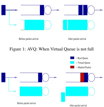
− Real Queue − Virtual Queue
Before packet arrival After packet arrival
Figure 1: AVQ: When Virtual Queue is not full
− Real Queue
Before packet arrival
After packet arrival − Virtual Queue − Marked Packet
Figure 2: AVQ: When the incoming packet is dropped from the Virtual Queue
2 The AVQ Algorithm
LetCbe the capacity of a link andγbe the desired utilization at the link. The AVQ scheme, as presented in [6, 7], at a router works as follows:
• The router maintains a virtual queue whose capacityC˜ ≤
Cand whose buffer size is equal to the buffer size of the
real queue. Upon each packet arrival, a fictitious packet is enqueued in the virtual queue if there is sufficient space in the buffer (See Figure 1). If the new packet overflows the virtual buffer, then the packet is discarded in the virtual buffer and the real packet is marked by setting its ECN bit or the real packet is dropped, depending upon the conges-tion notificaconges-tion mechanism used by the router (See Fig-ure 2).
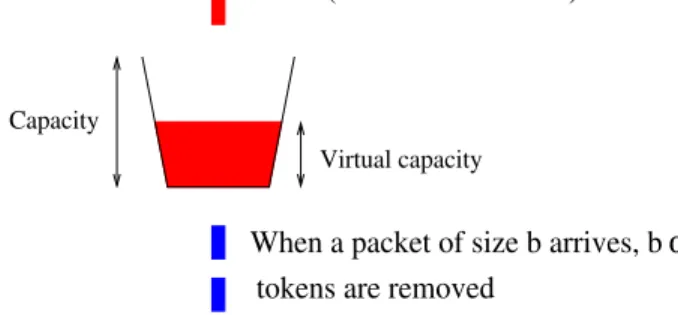
• At each packet arrival epoch, the virtual queue capacity is updated according to the following differential equation:
˙˜
C=α(γC−λ), (1)
where λ is the arrival rate at the link andα > 0 is the
smoothing parameter. The rationale behind this is that mark-ing has to be more aggressive when the link utilization ex-ceeds the desired utilization and should be less aggressive when the link utilization is below the desired utilization. We now make the following observations. No actual enqueue-ing or dequeueenqueue-ing of packets is necessary in the virtual queue, we just have to keep track of the virtual queue length. Equation (1) can be thought of as a token bucket where tokens are gener-ated at rateαγCup to a maximum ofCand depleted by each
arrival by an amount equal toαtimes the size of the packet (See Figure 3). Define
α
Capacity
Virtual capacity
Tokens are generated at the rate
tokens are removed
α
(Desired Utilization)
When a packet of size b arrives, b
Figure 3: AVQ: Token bucket implementation of the virtual ca-pacity adaptation
B=buffer size
s=arrival time of previous packet
t=Current time
b=number of bytes in current packet
V Q=Number of bytes currently in the virtual queue
Then, the following pseudo-code describes an implementa-tion of AVQ scheme:
The AVQ Algorithm At each packet arrival epoch do
V Q←max(V Q−C˜(t−s),0) /∗Update Virtual Queue Size∗/
IfV Q+b > B
Mark or drop packet in the real queue else
V Q←V Q+b /∗Update Virtual Queue Size∗/
endif
˜
C= max(min( ˜C+α∗γ∗C∗(t−s), C)−α∗b,0) /∗ Update Virtual Capacity∗/
s←t /∗Update last packet arrival time∗/
We note the following features of the AVQ scheme:
1. The implementation complexity of the AVQ scheme is com-parable to RED. RED performs averaging of the queue length, dropping probability computation and random num-ber generation to make drop decisions. We replace these with the virtual capacity calculation in AVQ.
2. AVQ is a primarily a rate-based marking, as opposed to queue length or average queue length based marking. This provides early feedback, the advantages of which have been explored by Hollot et al [4, 5], which was also mentioned in Kelly et al [15].
3. Instead of attempting to regulate queue length as in RED, PI controller or recent versions of REM, we regulate uti-lization. As we will see in simulations, this is more robust to the presence of extremely short flows or variability in the number of long flows in the network. The reason is that, when utilization is equal to one, variance introduced by the short flows seems to lead to an undesirable transient behav-ior where excessively large queue lengths persist over long
periods of time.
4. Unlike the GKVQ algorithm [11], we adapt the capacity of the virtual queue. A fixed value ofC˜ leads to a
utiliza-tion that is always smaller thanC/C˜ and it could be much
smaller than this depending on the number of users in the system. Our marking mechanism is also different in that we do not mark until the end of a busy period after a con-gestion episode.
5. There are two parameters that have to be chosen to imple-ment AVQ: the desired utilizationγand the damping
fac-torα. The desired utilizationγdetermines the robustness
to the presence of uncontrollable short flows. It allows an ISP to trade-off between high levels of utilization and small queue lengths. Both the parametersαandγdetermine the
stability of the AVQ algorithm and we provide a simple design rule to choose these parameters.
The starting point for the analysis of such a scheme is the fluid-model of the TCP congestion-avoidance algorithm as pro-posed in [6]. A theoretical justification of how a stochastic discrete-time equation can be approximated by a fluid-model is shown in [16]. We then incorporate the virtual capacity update equation with this model and study the stability of the entire system under linearization.
Consider a single link of capacityCwithNTCP users travers-ing it. Let the desired utilization of the link beγ≤1,and letd
be the round-trip propagation delay of each user (we assume that all users have the same round-trip propagation delay). Letxi(t)
be the flow-rate of useriat timet.We will model the TCP users using the −1
d2xutility function as proposed in [6]. For the sake of simplicity and tractability, we will neglect slow-start and time-outs when modeling the TCP users. We will later show through simulations that even with slow-start and timeouts, stability is maintained. Letp(., .)be the fraction of packets marked at the
link. The fraction of packets marked (i.e.,p(., .)) is a function of
the total arrival rate at the link as well as the virtual capacity of the link. The congestion-avoidance algorithm of TCP userican
now be represented by the following delay differential equation:
˙ xi= 1 d2 −βxi(t)xi(t−d)p( N X j=1 xj(t−d),C˜(t−d)), (2)
where β < 1 and C˜ is the virtual-capacity of the link. Aβ
value of2/3would give us the steady-state throughput of TCP
as 1 d
q
3
2p∗, where p
∗ is the steady-state marking probability which is consistent with the results in [17]. Hence, we will use
β = 2/3,in all our calculations. Also, note that on substituting
xi ≈Wdi,whereWiis the window-size of useri,we recover the
TCP window control algorithm [6, 3].
The update equation at each link can now be written as:
˙˜
C=α(γC−λ), (3)
whereλ = PN
j=1xj is the total flow into the link andα > 0
is the smoothing parameter. Note that αdetermines how fast
one adapts the marking probability at the link to the changing network conditions. We will present a design rule that specifies how to chooseαfor a given feedback delay (d), utilization (γ)
and a lower bound on the number of users (N). In fact, as we will show in Section 4, one can derive bounds on any of the four parametersα, γ, N ord,given the other three using the same design rule. However, in practice, it would seem most natural to chooseαgiven the other three parameters.
Letx∗
i,λ∗,C˜∗andp∗denote the equilibrium values ofxi,λ,
˜
Candp(λ,C˜).The equilibrium point of the non-linear TCP/AQM
model is given by:
X i x∗i = λ∗=γC x∗i = γC N p∗=p(γC,C˜∗) = N2 β(dγC)2.
Let us assume that
λ(t) = λ∗+δλ(t)
˜
C(t) = C˜∗+δC˜(t).
The linearized version of the non-linear TCP/AQM model can now be written as:
˙ δλ = −K11δλ(t)−K12δλ(t−d) +K2δC˜(t−d) (4) ˙ δC˜ = −αδλ(t), (5) where K11:= N γCd2, K12:= N γCd2 +β γC2 N ∂p(γC,C˜∗) ∂λ , and K2:=β γC2 N ∂p(γC,C˜∗) ∂C˜ .
For analytical tractability, we assume that
p(λ,C˜) = max{0,(λ−C˜)}
λ . (6)
We will now state themain resultof this paper which serves as the design for the AVQ algorithm. The proof of this result is given in Section 4.
Theorem 2.1 Suppose that the feedback delayd,number of users N,and the utilizationγ,are given. Letαˆbe given by:
ˆ α= min ( N γCd2, π 2dK2 r π2 4d2−K 2 12+K112 ) . (7) Then, for allα <α,ˆ the system is locally stable.
3 Simulations
The above theorem shows that by choosingαaccording to (7),
one can guarantee the local stability of the TCP/AQM scheme. However, the fluid-model does not take into account the discrete packet behavior of the network as well as the inherent nonlin-earities in the TCP algorithm. As a result, it becomes impor-tant to verify the analytical results using simulations in which
the nonlinearities of the system are taken into account. In this section, we conduct experiments that simulate various scenarios in the network and show that the AVQ algorithm performs as predicted by the analytical model in all the experiments. Even though each experiment shows that AVQ results in small queues, low loss and high utilization at the link, it is important to note that each experiment simulates a different scenario and the per-formance of AVQ is tested in this scenario.
In this section, we use the packet-simulatorns-2[18] to late the adaptive virtual queue scheme. We show that the simu-lation results agree with the convergence results shown in the previous section. In particular, we select an α, using
Theo-rem 2.1 that will ensure stability for a given round-trip delayd,
and a lower bound on the number of users,N.We then present
a single set out of many experiments that we did to show thatα
indeed stabilizes the system even in the presence of arrivals and departure of short connections. We then compare this scheme with many other AQM schemes.
3.1 Simulation Setup
Throughout this section, we consider a single link of capacity 10 Mbps that marks or drops packets according to some AQM scheme. For AVQ, unless otherwise stated, we letγ,the desired
utilization, be0.98.We use TCP-Reno as the default transport
protocol with the TCP data packet size set to 1000 bytes. Each TCP connection is placed in one of five classes which differ only in their round-trip propagation delays. Class 1 has a round-trip delay of 40 ms, Class 2 has a round-trip delay of 60 ms, Class 3 has a round-trip delay of 80 ms, Class 4 has a round-trip delay of 100 ms and Class 5 has a round-trip delay of 130 ms. The buffer size at the link is assumed to be100packets.
In the first five experiments, we assume that the link marks packets and thus, any packet loss is due to buffer overflow. In these experiments, we demonstrate that the AVQ scheme achieves high utilization and low packet loss. Further, the algorithm re-sponds quickly to changing network conditions such as vary-ing number of TCP flows. In the first experiment, we study the convergence properties of the AVQ algorithm both in the absence and in the presence of short flows. In the remaining experiments, we compare the AVQ algorithm with other AQM schemes like RED, REM, PI and the Gibbens’ and Kellys’ Vir-tual Queue (GKVQ). In the second experiment, we compare the performance of various AQM schemes in the presence of long-lived flows. In the third experiment, we compare the tran-sient behavior of the AQM schemes when long-lived flows are dropped and added to the network. In the fourth experiment, we compare the AQM schemes in the presence of short flows in the network. In the fifth experiment, we study the sensitivity of the AVQ algorithm to the smoothing parameter (α) as well as
to the desired utilization parameter (γ). In the last experiment,
we compare the AVQ scheme with other schemes when the link drops packets (as opposed to marking) to indicate congestion. Again, the AVQ scheme is shown to have smaller queue lengths compared to other schemes.
We design the AVQ controller for a maximum delay ofd = 350ms. Using the design rule in Theorem 2.1, anyα < 0.8,
non-0 20 40 60 80 100 120 140 160 180 200 450 500 550 600 650 700
Time (in seconds)
Virtual Capacity (in packets/second)
Virtual capacity vs time for AVQ
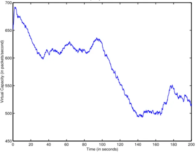
Figure 4: Experiment 1. Evolution of the virtual capacity with time for the AVQ scheme
Table 1: Experiment 1. Mean and the standard deviation of the queue size before and after the introduction of short flows.
Before After
Short Flows Short Flows Average Queue Size 12.17 19.19
Standard Deviation 10.28 13.44
linearities in the system, we letαbe0.15.In all experiments, we consider two types of flows: FTP flows that persist throughout the duration of the simulations and FTP flows of20packets each (to model the short flows).
Experiment 1:
In this experiment, we study the convergence properties and buffer sizes at the queue for the AVQ scheme alone. A total of180FTP flows with36in each delay class persist throughout
the duration of the simulations, while short flows (of20
pack-ets each) arrive at the link at the rate of30flows per second.
The short flows are uniformly distributed among the five delay classes. To simulate a sudden change in network conditions, we start the experiment with only FTP flows in the system and intro-duce the short flows after100seconds. The evolution of the vir-tual capacity is given in Figure 4. After an initial transient, the virtual capacity settles down and oscillates around a particular value. Note that the oscillations in the virtual capacity are due to the packet nature of the network which is not captured by the analytical model. At 100 seconds, there is a drop in the virtual capacity since the AVQ algorithm adapts to the changing num-ber of flows. Beyond 100 seconds, the virtual capacity is lower than it was before 100 seconds since the links marks packets ag-gressively due to the increased load. The queue length evolution for the system every100ms is given in Figure 5. Except
dur-ing transients introduced by load changes, the queue lengths are small (less than 20 packets). At 100 seconds, the queue length jumps up due to the short flows. However, the system stabilizes and the queue lengths are small once again. Table 1 gives the average and the standard deviation of the queue length before and after the introduction of short flows. Note that there is
0 20 40 60 80 100 120 140 160 180 200 0 10 20 30 40 50 60 70 80 90
Time (in seconds)
Queue length (in packets)
Queue length vs time for AVQ
Figure 5: Experiment 1. Queue length vs time for the AVQ scheme
a small increase in the average queue length as well as in the standard deviation due to the addition of short-flows in the sys-tem. Another important performance measure is the number of packets dropped due to buffer overflow in the system. Since ECN marking is used, we expect the number of packets lost due to buffer overflow to be small. Indeed only10out of roughly 250,000packets are dropped. These drops are primarily due to
the sudden additional load brought on by the short flows. An-other performance measure that is of interest is the utilization of the link. The utilization was observed to be0.9827,which
is very close to the desired utilization of0.98.We note that the
apparent discrepancy between Figure 5, where the queue length never reaches the buffer size of100 packets, and the fact that
there are 10dropped packets is due to the fact that the queue length is sampled only once every100 ms to plot the graphs. We will now compare the AVQ scheme with other AQM schemes that have been proposed. Since there are many AQM schemes in the literature, we will compare the AVQ scheme with a rep-resentative few. In particular, we will compare the AVQ scheme with
1. Random Early Discard (RED) proposed in [1]. In our ex-periments, we use the “gentle” version of RED. Unless oth-erwise stated, the parameters were chosen as recommended inhttp://www.aciri.org/floyd/REDparameters.txt.
2. Random Early Marking (REM) proposed in [10]. The REM scheme tries to regulate the queue length to a desired value (denoted by qref) by adapting the marking probability. The REM controller marks each packet with a probabil-itypwhich is updated periodically (say, everyT seconds)
as
p[k+ 1] = 1−φ−µ[k+1],
whereφis a arbitrary constant greater than one and µ[k+1] = max(0, µ[k]+γ(q[k+1]−(1−α)q[k]−αqref)),
andαandγare constants andq[k+ 1]is the queue length
at thek+ 1sampling instant. Since REM is very sensitive toφ,we will use the values as recommended in [10].
3. The PI controller proposed in [5]. The PI controller marks each packet with a probabilitypwhich is updated periodi-cally (say, everyT seconds) as
p[k+ 1] =p[k] +a(q[k+ 1]−qref)−b(q[k]−qref),
wherea > 0andb >0are constants chosen according to the design rules given in [5].
4. The virtual queue based AQM scheme (GKVQ) proposed in [11]. In this scheme, the link maintains a virtual queue with fixed capacity C˜ = θC, and buffer size B˜ = θB,
whereθ <1,andB is the buffer capacity of the original
queue. Whenever the virtual queue overflows, all pack-ets in the real queue and all future incoming packpack-ets are marked till the virtual queue becomes empty again. Note that this scheme cannot be used in the case where the link drops the packets instead of marking them because the through-put would be very bad due to aggressive dropping. As in [11], we will useθ = 0.90in all our simulations using the GKVQ.
Experiment 2:
In this experiment, we compare the performance of the various AQM schemes assuming that the link “marks” packets and in the presence of long-lived FTP flows only. The queue size at the link is set to 100 packets. The desired queue length for the REM scheme and the PI scheme is set at50packets and the minthresh and the maxthresh for the RED (with gentle turned on) scheme are set at37and75packets respectively. Recall that the desired utilization of the link is set to be0.98for the AVQ scheme.
Since we use an average queue length of50packets for REM
and the PI controller, it is natural to attempt to regulate the queue length to50for the AVQ scheme also. However, the AVQ does
not directly attempt to control queue size. Thus, for the AVQ scheme, we drop every packet that arrives when there are al-ready 50 packets in the real queue. Note that this is the worst-case scenario for the AVQ scheme, since when ECN marking is used, the natural primary measure of performance is packet loss.
We summarize our simulation results below:
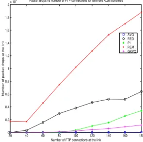
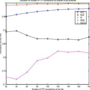
• Packet Losses and Link Utilization: The losses incurred by all the schemes are shown in Figure 6 as a function of the number of FTP flows. The AVQ scheme has fewer losses than any other scheme except the GKVQ even at high loads. The loss rate for GKVQ and AVQ are com-parable; however, the GKVQ marks packets more aggres-sively than any other scheme and thus has lower utilization. Figure 7 shows the utilization of the link for all the AQM schemes. Note that, the utilization of GKVQ is as low as
75%.This can once again be attributed to the aggressive
marking strategy of GKVQ. RED also results in a poor uti-lization of the link. Our observation has been that when in-creasing the utilization of RED (by tuning its parameters), the packet losses at the link also increases. REM and PI have a utilization of 1.0 as the queue is always non-empty. For the AVQ scheme, we required a desired utilization of 0.98 and we can see that the AVQ scheme tracks the desired utilization quite well. Thus, the main conclusion from this experiment is that the AVQ achieves low loss with high uti-lization. 20 40 60 80 100 120 140 160 180 0 0.2 0.4 0.6 0.8 1 1.2 1.4 1.6 1.8 2x 10 4
Number of FTP connections at the link
Number of packet drops at the link
Packet drops vs number of FTP connections for different AQM schemes
AVQ RED PI REM GKVQ
Figure 6: Experiment 2. Losses at the link for varying number of FTP connections for the different AQM schemes
• Responsiveness to changing network conditions: The objec-tive of this experiment is to measure the response of each AQM scheme when the number of flows is increased. Twenty new FTP users are added every 100s till the total num-ber of FTP connections reach 180 and the average queue length over every 100s is computed. Schemes that have a long transient period will have an increasing average queue length as new users are added before the scheme is able to converge. The average queue length (over each100second interval) of each scheme as the number of users increase is shown in Figure 8. We see from the figure that PI and REM have higher average queue lengths than the desired queue length. On the other hand, AVQ, GKVQ and RED have smaller queue sizes. This is due to the fact that REM and PI apparently have a long transient period and new users are added before the queue length converges. The aver-age queue length over each100s interval is used to capture
persistent transients in this experiment for studying the re-sponsiveness of the AQM schemes to load changes. This experiment shows that AVQ is responsive to changes in network load and is able to maintain a small queue length even when the network load keeps increasing.
Experiment 3:
In this experiment, we compare the responsiveness of the AQM schemes when flows are dropped and then introduced later on. Specifically, we only compare REM and the PI controller (since these are only ones among those that we have discussed that attempt to precisely regulate the queue length to a desired value) with the AVQ controller. Unless otherwise stated, all the system parameters are identical to Experiment 2. The number of FTP connections is 140 at time0.0At time100,105FTP connections
are dropped and at time150a new set of105FTP connections
is established. We plot the evolution of the queue size for each of the AQM scheme. Figure 9 shows the evolution of the queue size for PI as the flows depart and arrive. Note that the desired
20 40 60 80 100 120 140 160 180 0.7 0.75 0.8 0.85 0.9 0.95 1
Number of FTP connections at the link
Utilization at the link
Utilization vs number of FTP connections for different AQM schemes
AVQ RED PI REM GKVQ
Figure 7: Experiment 2. Achieved Utilization at the link for the different AQM schemes
20 40 60 80 100 120 140 160 180 0 10 20 30 40 50 60 70 80 90 100
Number of FTP connections at the link
Average queue length in packets
Average queue length vs number of FTP connections for different AQM schemes
AVQ RED PI REM GKVQ
Figure 8: Experiment 2. Queue length at the link for varying number of FTP connections for the different AQM schemes
0 50 100 150 200 250 0 10 20 30 40 50 60 70 80 90 100 Time in seconds
Queue length in packets
Queue length vs time for PI with 140 FTP connections
PI
Figure 9: Experiment 3. Evolution of the queue length at vary-ing loads for PI
0 50 100 150 200 250 0 10 20 30 40 50 60 70 80 90 100 Time in seconds
Queue length in packets
Queue length vs time for AVQ with 140 FTP connections
Figure 10: Experiment 3. Evolution of the queue sizes at vary-ing loads for AVQ
0 50 100 150 200 250 0 10 20 30 40 50 60 70 80 90 100 Time in seconds
Queue length in packets
Queue length vs time for REM with 140 FTP connections
REM
Figure 11: Experiment 3. Evolution of the queue sizes at vary-ing loads for REM
queue length is 50packets. We can see that the system takes
some time to respond to departures and new arrivals. On the other hand, the queue in the AVQ scheme in Figure 10 responds quickly to the removal of flows at time t = 100, and to the
addition of flows at time150.Figure 11 gives the evolution of
the queue sizes for REM. The desired queue level in the REM scheme is50packets and REM is very slow to bring the queue
level to50packets. On removing flows, the queue level drops, but on addition of new flows, there is a large overshoot in REM.
Experiment 4:
Till now we have been comparing AVQ and all other AQM schemes in the absence of short flows. However, a large part of the connections in the Internet comprise of short flows. As a result, it is important to study the performance of an AQM scheme in the presence short flows. In this experiment, we will start with 40 FTP connections that persist throughout the length of the experiment. We also allow the AQM schemes to converge to the optimal solution when there are only 40 FTP connections in the network. We then introduce short flows and study the performance of the AQM scheme as the number of short flows increases. We start with a short-flow arrival rate of 10 per sec-ond and gradually increase it to 50 short flows per secsec-ond. Each short flow transfers 20 packets using TCP/Reno. The round-trip
0 5 10 15 20 25 30 35 40 45 50 0 1000 2000 3000 4000 5000 6000 7000 8000 9000 10000
Number of short flows arriving per second at the link
Number of packet drops at the link
Number of packets dropped vs number of short flows for different AQM schemes AVQ RED PI REM GKVQ
Figure 12: Experiment 4. Packet losses at the link for various AQM schemes
times of the short flows are also distributed uniformly between the five delay classes.
We again study the following performance measures: • Packet losses and Utilization: The losses incurred by all the
schemes are shown in Figure 12. Note that AVQ has lower drops than the RED, REM and the PI schemes. GKVQ in-curs no significant packet drops (and hence cannot be seen in the figure) because of its aggressive marking scheme. However, as in Experiment 2, the utilization of GKVQ is poor as seen in Figure 13. We again see that REM and PI have a utilization of one, while RED and GKVQ have poor utilization. For the AVQ scheme, the utilization is actually slightly higher than the desired utilization at high loads, but this can be attributed to the load brought by the short-flows. From this experiment, we can see that AVQ has lower drops compared to REM, PI and RED in the pres-ence of short flows. Even though, AVQ has more drops than GKVQ, the utilization at the link for AVQ is signifi-cantly greater than the GKVQ algorithm.
• Queue length: The average queue length of each scheme as the rate of the incoming short-flows short connections are increased is shown in Figure 14. We see that the AVQ controller maintains the smallest queue length among all schemes as the number of short-flows increases.
Experiment 5:
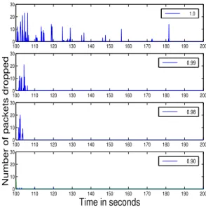
In this experiment, we study the sensitivity of the AVQ algo-rithm to the smoothing parameter (α) and the desired utilization
parameter (γ). The number of long TCP connections accessing
the link is fixed at180and the simulation setup is identical to
that in Experiment 1. From Theorem 2.1, any value ofα≤0.8
will guarantee stability. In addition to the long flows, short flows are introduced after100s.In the first part of the experiment, the
smoothing parameter,α,is varied from0.20to0.80,while the
desired utilization parameter,γ,is fixed at0.98.The evolution of the queue length is shown in Figure 15. We can see that the
0 5 10 15 20 25 30 35 40 45 50 0.7 0.75 0.8 0.85 0.9 0.95 1
Number of short flows arriving per second at the link
Utilization at the link
Utilization for varying number of short flows for different AQM schemes AVQ RED PI REM GKVQ
Figure 13: Experiment 4. Utilization of the link for various AQM schemes 0 5 10 15 20 25 30 35 40 45 50 0 10 20 30 40 50 60 70 80 90 100
Number of short flows arriving per second at the link
Average queue length in packets
Average queue length for varying number of short flows for different AQM schemes
AVQ RED PI REM GKVQ
Figure 14: Experiment 4. Average queue length at the link for various AQM schemes
average queue lengths remain small irrespective of the value of
αthat is used. However, the transients due to the sudden load of the short flows att = 100sis more pronounced whenαis small. Hence, even though a very small value ofαcan
guaran-tee stability, it can make the link sluggish to changes in network load. A theoretical analysis of the transient behavior is required to precisely quantify the impact ofαon the system performance.
This could be a topic for future research.
In the second part of the experiment, we fix the value ofαto
be equal to0.5 and vary the value ofγ.We use four different
values ofγ(0.90,0.98,0.99and1.0) to study the sensitivity of
the algorithm toγ.The rest of the simulation setup is identical
to the first part. We increase the burstiness of the short flows by splitting a single short flow of20packets into two short flows
0 20 40 60 80 100 120 140 160 180 200 0 50 100 0.20 0 20 40 60 80 100 120 140 160 180 200 0 50 100 0.40 0 20 40 60 80 100 120 140 160 180 200 0 50 100
Queue size in packets
0.60 0 20 40 60 80 100 120 140 160 180 200 0 50 100 Time in seconds 0.80
Figure 15: Experiment 5. Evolution of the queue length for different values of the smoothing parameterα
of10packets each. Figure 16 shows the evolution of the queue
length for the different values ofγ.We can see that smaller
val-ues ofγresults in smaller queue sizes. As a result, smaller
val-ues ofγresults in smaller number of dropped packets as shown
in Figure 17. Note that whenγ < 1,packet drops are primar-ily caused by the sudden load change at100s.After a transient period in which the algorithm tries to adapt to the new load, there are no more packet drops. But the duration of the tran-sient period seems to increase asγis increased. Whenγ = 1,
the transients caused by new short flows is sufficient to cause buffer overflow in certain instances. The achieved utilization (averaged over one second) is shown in Figure 18. We can see that irrespective of the value ofγ,AVQ tracks the desired
uti-lization quite well. For a desired average queue length (or loss probability), an upper bound on the value ofγ would depend
on the traffic characteristics. Given the traffic characteristics, desired loss probability or desired average queue length, analyt-ically computing an appropriate value forγis a topic for future
research.
Experiment 6:
Till now, we have assumed that the router marks packets upon detecting congestion. Instead one can drop packets when con-gestion is detected. In this experiment, we use dropping instead of marking when the links detects an incipient congestion event. Note that, in the case of marking, the main goal of the adap-tive algorithm was to match the total arrival rate to the desired utilization of the link. However, in the case of dropping, the link only serves those packets that are admitted to the real queue. As a result, in the case of dropping, one adapts the virtual capacity (C˜) only when a packet has been admitted to the real queue, i.e.,
only the accepted arrival rate is taken into consideration. We compare RED, REM and PI controller to the AVQ scheme. We do not use GKVQ as a dropping algorithm as the number of packets dropped on detecting congestion would be very high and it would result in negligible throughput. The buffer limit at the link is set to 100 packets. The users employ TCP NewReno.
0 20 40 60 80 100 120 140 160 180 200 0 50 100 1.0 0 20 40 60 80 100 120 140 160 180 200 0 50 100 0.99 0 20 40 60 80 100 120 140 160 180 200 0 50 100
Queue size in packets
0.98 0 20 40 60 80 100 120 140 160 180 200 0 50 100 Time in seconds 0.90
Figure 16: Experiment 5. Evolution of the Queue Length for different values ofγ 100 110 120 130 140 150 160 170 180 190 200 0 10 20 30 1.0 100 110 120 130 140 150 160 170 180 190 200 0 10 20 30 0.99 100 110 120 130 140 150 160 170 180 190 200 0 10 20 30
Number of packets dropped
100 110 120 130 140 150 160 170 180 190 200 0 10 20 30 Time in seconds 0.98 0.90
Figure 17: Experiment 5. Number of Dropped packets vs Time for different values ofγ
All the other parameters are as in Experiment 2. However, in this case we simulate the AVQ scheme with bothγ = 1.0and
γ = 0.98.The reason for usingγ = 0.98earlier was to have small losses to get the most benefit from ECN marking. Since marking is no longer used, we also study the AVQ under full utilization.
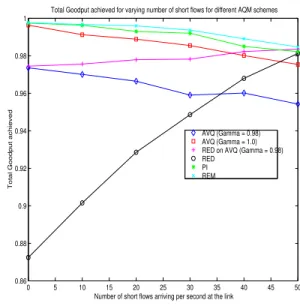
We have 40 FTP connections traversing the link for the en-tire duration of the simulation. We allow the respective AQM schemes to converge and then introduce short-flows at 100s. Short-flows introduced are TCP-RENO sources with 20 pack-ets to transmit. The rate at which short flows arrive at the link is slowly increased. The average queue length, and the utiliza-tion are shown in Figure 19 and Figure 20. The total goodput is shown in Figure 21. By goodput, we mean the number of
0 20 40 60 80 100 120 140 160 180 200 0.85 0.9 0.95 1 1.05 Time in seconds 0 20 40 60 80 100 120 140 160 180 200 0.85 0.9 0.95 1 1.05 Achieved Utilization 0.98 0 20 40 60 80 100 120 140 160 180 200 0.85 0.9 0.95 1 1.05 0.99 0 20 40 60 80 100 120 140 160 180 200 0.85 0.9 0.95 1 1.05 1.0 0.90
Figure 18: Experiment 5. Achieved Utilization vs Time for dif-ferent values ofγ 0 5 10 15 20 25 30 35 40 45 50 0 10 20 30 40 50 60 70 80 90 100
Number of short flows arriving per second at the link
Average queue length in packets
Average queue length for varying number of short flows for different AQM schemes AVQ (Gamma = 1.0)
AVQ (Gamma = 0.98) RED PI REM
Figure 19: Experiment 6. Average queue lengths for various AQM schemes
packets successfully delivered by the link to the TCP receivers. In general, this could be different from the throughput (which is the total number of packets processed by the link) due to TCP’s retransmission mechanism. Note that the average queue length, the goodput of each flow and fairness are the three possible performance objectives that one would use to compare differ-ent AQM schemes when dropping is employed as a congestion notification mechanism. In practice, we would like an AQM scheme that maintains a small average queue length with high utilization. However, the AQM scheme should not introduce any additional bias in the rates towards smaller round-trip flows (TCP by itself introduces a bias towards smaller round-trip flows and we do not want to add it). In this experiment, we compared the average queue length and the utilization at the link of AVQ,
0 5 10 15 20 25 30 35 40 45 50 0.91 0.92 0.93 0.94 0.95 0.96 0.97 0.98 0.99 1 1.01
Number of short flows arriving per second at the link
Utilization at the link
Utilization for varying number of short flows for different AQM schemes
AVQ (Gamma = 1.0) AVQ (Gamma = 0.98) RED PI REM
Figure 20: Experiment 6. Utilization for various AQM schemes
0 5 10 15 20 25 30 35 40 45 50 0.86 0.88 0.9 0.92 0.94 0.96 0.98 1
Number of short flows arriving per second at the link
Total Goodput achieved
Total Goodput achieved for varying number of short flows for different AQM schemes
AVQ (Gamma = 0.98) AVQ (Gamma = 1.0) RED on AVQ (Gamma = 0.98) RED PI REM
Figure 21: Experiment 6. Total Goodput for the various AQM schemes
RED, REM and PI.
Note: Instead of marking or dropping a packet in the real queue when the virtual queue overflows, one can mark or drop packets in the real queue by applying RED (or any other AQM algorithm) in the virtual queue. Thus, if there are desirable fea-tures in other AQM schemes, they can be easily incorporated in the AVQ algorithm. When marking is employed, our expe-rience is that a simple mark-tail would be sufficient as shown in Experiments 1 through 4. In the case when the link drops the packets, many successive packet drops from the same flow could cause time-outs. To avoid this, one could randomize the dropping by using a mechanism like RED in the virtual queue to prevent bursts of packets of the same flow to be dropped. Hence, in this experiment, we also consider an AVQ scheme that had RED implemented in its virtual queue.
Our experience has been that, if RED is employed in the vir-tual queue, the performance of the AQM scheme is not very sen-sitive to the choice of the RED parameters. Even though, there is no significant difference in the goodputs, we believe that the fairness of the AVQ scheme can be improved using a proba-bilistic dropping scheme in the virtual queue at the expense of increased computation at the router. We intend to study the fair-ness properties in our future research work. Note that a proba-bilistic AQM scheme on the virtual queue is required only when the link drops packets and not when the link marks packets be-cause multiple marks within a single window does not be-cause TCP to time-out or go into slow-start.
4 Stability Analysis of the AVQ scheme
In this section, we will prove the main result of the paper which was stated in Theorem 2.1. The starting point of the analysis is the linearized version of the TCP/AQM model derived in (4) and (5). We summarize the main ideas behind the proof:
• The stability of a linear delay-differential equation can be analyzed using its characteristic equation. The character-istic equation of the linear delay-differential equation can be obtained by taking its Laplace Transform. For the lin-earized system to be stable, its characteristic equation should have all its roots in the left-half plane (i.e., ifσis a root of the characteristic equation, then Re[σ]<0).
• We will first show that forα, N,andγfixed, the system is stable in the absence of feedback delays, i.e.,d= 0.This implies that all the roots of the characteristic equation lie in the left-half plane. The roots of the characteristic equation are continuous functions of its parameters. Therefore, the roots of the characteristic equation are continuous function of the feedback delayd.By increasingd,one can find the
smallest feedback delayd∗ at which one of the roots hits the imaginary axis (if there is no suchd,then the system is
stable for alld.). Hence, for alld < d∗, the system has all its roots in the left-half plane and hence it is stable. This is the key idea behind the stability analysis in this section. Recall that the linearized TCP/AQM system was given in (4) and (5). For analytical tractability, we assume that
p(λ,C˜) =Max{0,(λ−C˜)}
λ . (8)
Note that, while this is not differentiable everywhere inλorC˜, it
is differentiable in the regionλ >C.˜ Substituting for∂p(γC,∂λC˜∗),
and∂p(γC,C˜∗)
∂C˜ and using the fact thatp(γC,C˜
∗) = N2 β(dγC)2,we find that K11= N γCd2 K12=K2=β γC N . (9)
Note thatK12 > K11.LetΛ(s)denote the Laplace-Transform
ofδλ(t)and letΨ(s)denote the Laplace-transform ofδC˜(t).
Taking the Laplace-transforms of (4) and (5), we get:
sΛ(s) =−K11Λ(s)−K12e−sdΛ(s) +K2e−sdΨ(s) (10)
sΨ(s) =−αΛ(s). (11)
Substituting (11) in (10), we get the so-called characteristic equa-tion s+K11+e−sd K12+αK2 s = 0. (12)
Next, we use the fact that the roots are continuous functions of the round-trip delayd.As a result, if the system is stable with
d = 0for a fixed value ofα,then the roots are strictly in the left-half plane. Therefore, we can choosedsmall enough such that the roots still remain in the left-half plane. This will help us to find the maximum feedback delay for which the system is stable for a givenα.We will then show that we can use the
same technique to show that given a feedback delayd,one can
find the maximum value ofαfor which the system is stable. We
will formalize these ideas in this section.
Whend = 0,i.e., there is no feedback delay in the system,
the characteristic equation reduces to:
s+K11+K12+α
K2
s = 0. (13)
Solving the quadratic equation, we get:
s= −(K11+K12)±
p
(K11+K12)2−4αK2
2 .
If4αK2 ≤ (K11 +K12)2, then the system has all real roots
which lie strictly in the left half-plane. If 4αK2 > (K11+
K12)2,then the system has complex roots that also lie strictly in
the left half-plane. Thus, for all values ofα > 0,the system is stable.
The following theorem gives the necessary condition on the RTT for the stability of the system given by (4) and (5). Theorem 4.1 Fixα= ˆα,the number of TCP users,N and the
utilizationγ.Find the smallestd= ˆdsuch that ω(ˆα, d, N, γ) = s (K2 12−K112 ) + p (K2 12−K112)2+ 4K22αˆ2 2 (14) satisfies ωd+ arctan αˆ ω + arctan ω K11 = (2k+ 1)π, (15) for somek = 0,1,2,· · ·.Then, the TCP/AQM system given in
(4) and (5) is stable for all values ofd <d.ˆ
Proof:The characteristic equation of the TCP/AQM system (12) can be rewritten as:
1 +e
−sd K
12+αKs2
s+K11
= 0. (16)
Letjω be one of the roots of the characteristic equation at the smallest d = d∗ such that the roots hits the imaginary axis. Since the roots on the imaginary axis are complementary, we will concern ourselves only withω≥0.From (16), we get:
e−jωdK
12+αKjω2
jω+K11
To satisfy the last condition, the following conditions must be met simultaneously: Condition on magnitude: e−jωdK 12+αKjω2 jω+K11 = 1 Condition on angles: 6 e−jωdK 12+αKjω2 jω+K11 = (2k+ 1)π k= 0,±1,±2.
From the condition on magnitude, we get
q K2 12+ K2 2αˆ2 ω2 p K2 11+ω2 = 1 (or) ω( ˆα, d, N, γ) = r (K2 12−K112) + p (K2 12−K112 )2+ 4K22αˆ2 2 . (17)
From the condition on angles, we get:
ωd+ arctan αˆ ω + arctan ω K11 = (2k+ 1)π,
fork= 0,1,2,· · ·.SinceK11is a decreasing function ofd,and
K12 andK2 are independent ofd,we note thatω(ˆα, d, N, γ)
is an increasing function ofd.Therefore, the smallest d = ˆd
that solves (15) gives the smallest delay such that at least one of the roots hits the imaginary axis. Therefore, for alld < d,ˆ the
system is locally asymptotically stable.
REMARK:Although Theorem 4.1 provides a necessary and sufficient condition, it is hard to verify the conditions of the the-orem numerically due to the following issues:
• What value ofkwill yield the smallestd?
• Ifdˆsolves (15), how can we be sure that there exists nod,˜
such thatd˜solves (15) andd <˜ dˆ?
Theorem 4.2 solves these issues by giving an easily verifiable sufficient condition for stability. Before stating the theorem, we state the following useful fact:
Fact 4.1 Letaandbbe arbitrary positive constants witha≤b.
Then, max x arctan( a x) + arctan( x b) = π 2. (18)
Theorem 4.2 Fixα= ˆα,the number of TCP users,N and the utilizationγ.Definedˆto be:
ˆ d= min{ s N γCαˆ, d ∗ }, (19) whered∗solves: ωd∗=π 2, (20)
andωis as given in (14). Then for alld <dˆthe system is stable. Moreover,d∗is unique.
Proof:Note thatK12andK2do not depend ond.Also,K11= N
γCd2.Therefore, asdincreases,K11decreases andωincreases. Note that we can easily show thatd∗is a unique solution to (20). Also, note thatdˆ≤d∗.Hence,
ωdˆ≤ π2.
Letd˜solve (15) for somek.Then, we claim that ˆ
d <d.˜ (21)
Suppose not. Sincedˆ2< N
γCαˆandd <˜ d,ˆwe haveα < Kˆ 11( ˜d).
Thus, using Fact 4.1,
arctan(αˆ ω) + arctan( ω K11 )≤ π2. Therefore, ω(ˆα,d, N, γ˜ ) ˜d≥4k2+ 1π, k= 0,1,2. . . (22)
Also, sinced <˜ d, ωˆ (ˆα,d, N, γ˜ )< ω(ˆα,d, N, γˆ ).Thus, ω(ˆα,d, N, γ˜ ) ˜d < ω(ˆα,d, N, γˆ ) ˆd≤π
2.
But this contradicts (22). Hencedˆ≤ d.˜ Thus, anyd < dˆalso
satisfiesd <d,˜and therefore, for anyd <d,ˆthe system is stable
from Theorem 4.1.
Till now, we have been given a fixedαand a fixedN and we
were interested in finding the largest feedback delay for which this system is stable. But, a more practical question is the fol-lowing: given a feedback delayd,˜ and number of usersN,how
can one designαsuch that the system is stable? The next theo-rem gives a method by which one can designαsuch that system is stable. Note that this theorem is the main result of the paper and is also stated in Section 2. We state it again for convenience. Theorem 4.3 Suppose that the feedback delayd,ˆnumber of users
ˆ
N ,and the utilizationˆγ,are given. Letαˆbe given by: ˆ α= min N γCdˆ2, π 2 ˆdK2 s π2 4 ˆd2 −K 2 12+K112 . (23) Then, for allα <α,ˆ the system is locally stable.
Proof:Using (20), we know that
ˆ
dω(ˆα,d,ˆN ,ˆ γˆ)≤ π2.
Now let us fix anα <˜ α.ˆ Since,α <˜ α,ˆ we have:
˜
α < K11(d), ∀d≤d,ˆ
and
ω(˜α, d,N ,ˆ γˆ)< ω(ˆα, d,N ,ˆ γˆ)< ω(ˆα,d,ˆN ,ˆ γˆ) ∀d≤d.ˆ
Therefore, using Fact 4.1 we get for alld≤dˆ: dω( ˜α, d,N ,ˆ ˆγ) + arctan( αˆ
ω( ˜α, d,N ,ˆ ˆγ)) + arctan(
ω( ˜α, d,N ,ˆ ˆγ)
K11(d)
< π. Hence, the system is stable for allα <α.ˆ
Theorem 4.4 Fix the feedback delayd,˜ the number of usersN
and the utilizationγ.Findα∗satisfying:
ωd˜+ arctan ω K11 =π 2, (24)
whereωis as given in (14). Then, for allα < α∗,the system is stable.
We will now show that if there exists anα >ˆ 0that satisfies
(24), then there exists anα∗>0that satisfies (23).
Theorem 4.5 Fix the feedback delayd,ˆ the number of usersNˆ
and the utilizationγ.ˆ Letα >ˆ 0solve (24). Then there exists an
α∗>0that satisfies (23).
Proof: Suppose there does not exist anα∗ > 0that satisfies (23). This implies
K122 −K112 >
π2
4 ˆd2. (25)
However, there exists anαˆsuch that:
ˆ dω(ˆα,d,ˆN ,ˆ γˆ) =π 2 −arctan( ω(ˆα,d,ˆN ,ˆ γˆ) K11 ). Let κ= arctan(ω(ˆα,d,ˆN ,ˆ γˆ) K11 )>0. Therefore, ˆ dω(α,d,ˆN ,ˆ γˆ) =π−2κ 2 .
From (17), we know that
K122 −K112 <(ω(α,d,ˆN ,ˆ ˆγ))2. Therefore, K122 −K112 < (π−2κ)2 4 ˆd2 < π2 4 ˆd2.
This contradicts (25). Hence, there exists aα∗that satisfies (23). Example 4.1 In this example, we will compare the value ofα
obtained from (24) and (23). In particular, we will show that one might not be able to solve (24) even though one can solve (23). Consider a single link with 10Mbps capacity and let there be150users accessing it. Using an average packet size of 1000
bytes, the capacity of the link can be written as1250packets per second. Let the desired utilization at the linkγto be0.98.Let
˜
d= 0.15.Using (24) we compute the value ofαˆ= 4.7710. Us-ing (23) to solve forα∗,we getα∗ = 5.44.Now, if we increase the delay to0.25seconds, there exists noαˆthat will solve (24). However, using (23) to solve forα∗,we getα∗= 1.95.In view of this example and the previous theorem, (23) is a less restric-tive condition onαthan (24).
The next theorem quantifies the impact ofN,the number of users, on the stability of the system.
Theorem 4.6 Fix the feedback delayd,ˆ the smoothing parame-terαˆand the utilizationγ.DefineNˆ to be:
ˆ
N = max{αˆdˆ2γC, N∗}, (26) whereN∗satisfies:
ωdˆ= π 2,
andωis as given in (14). Then, for allN > N ,ˆ the system is stable.
Proof:Note that in this case,K11,K12,andK2are all functions
ofN.We can easily show that asN increases, K11increases,
K12decreases,K2decreases andω(α, d, N, γ)decreases.
Us-ing this and followUs-ing along the lines of the proof for Theo-rem 4.3, we can show that for allN >N ,ˆ the system is locally
stable.
A similar theorem can now be stated forγ.
Theorem 4.7 Fix the feedback delayd,ˆnumber of usersNˆ and
the smoothing parameterα.ˆ Defineˆγto be:
ˆ γ= min{ N Cdˆ2αˆ, γ ∗}, (27) whereγ∗solves: ωdˆ= π 2,
andω is as given in (14). Then, for all γ < γ,ˆ the system is
stable.
5 Conclusions
Robust Active Queue Management schemes at the routers is es-sential for a low-loss, low-delay network. In this paper, an easily implementable robust AQM scheme called theAdaptive Virtual Queue (AVQ)algorithm is presented. The implementation com-plexity of the AVQ algorithm is comparable to other well-known AQM schemes. While the present form of AVQ adapts the vir-tual capacity on every packet arrival, an acvir-tual implementation in routers might perform this adaptation everyKpackets (as in
the PI controller [4]). Parameter choice for AVQ in this scenario is a topic for future research.
In this paper, we provide simple design rules to choose the smoothing parameters of the AVQ algorithm. The criterion we use to choose the parameters is local stability of the congestion-controllers and the AQM scheme together. However, it would also be useful to quantify the impact of the desired utilization
γon QoS parameters such as loss probability or average queue
length. This is a topic for future research.
We show through simulations that the AVQ controller out per-forms a number of other well-known AQM schemes in terms of losses, utilization and average queue length. In particular, we show that AVQ is able to maintain a small average queue length at high utilizations with minimal loss at the routers. This con-clusion also holds in the presence of short flows arriving and de-parting at the link. We also show that AVQ responds to changing network conditions better than other AQM schemes (in terms of average queue length, utilization and losses).
We also study the performance of AVQ when dropping (in-stead of marking) is employed at the routers. While AVQ per-forms better than other AQM schemes in terms of utilization and average queue length, the fairness of AVQ can be improved us-ing a probabilistic AQM scheme (like RED) on AVQ. We note that a probabilistic AQM scheme on the virtual queue is required only when the link drops packets and not when the link marks packets because multiple marks within a single window does not cause TCP to time-out or go into slow-start. The fairness prop-erties of AVQ with packet dropping is a topic of future research. An important feature of the AVQ algorithm is that one can employ any AQM algorithm in the virtual queue. Thus, if there are desirable properties in any other marking schemes, one can easily incorporate it into the AVQ scheme. However, when marking is employed, our experience has been that a simple mark-tail would suffice.
References
[1] S. Floyd and V. Jacobson, “Random early detection gate-ways for congestion avoidance,” IEEE/ACM Transactions on Networking, August 1993.
[2] S. Floyd, “TCP and explicit congestion notification,”ACM Computer Communication Review, vol. 24, pp. 10–23, Oc-tober 1994.
[3] V. Misra, W. Gong, and D. Towlsey, “A fluid-based anal-ysis of a network of AQM routers supporting TCP flows with an application to RED,” in Proceedings of SIG-COMM, Stockholm, Sweden, September 2000.
[4] C.V. Hollot, V. Misra, D. Towlsey, and W. Gong, “On de-signing improved controllers for AQM routers supporting TCP flows,” inProceedings of INFOCOM, Alaska, An-chorage, April 2001.
[5] C.V. Hollot, V. Misra, D. Towlsey, and W. Gong, “A con-trol theoretic analysis of RED,” inProceedings of INFO-COM, Alaska, Anchorage, April 2001.
[6] S. Kunniyur and R. Srikant, “End-to-end congestion con-trol: utility functions, random losses and ECN marks,” in Proceedings of INFOCOM, Tel Aviv, Israel, March 2000. Also to appear inIEEE/ACM Transactions on Networking, 2003.
[7] S. Kunniyur and R. Srikant, “A time-scale decomposition approach to adaptive ECN marking,” IEEE Transactions on Automatic Control, June 2002.
[8] T. J. Ott, T. V. Lakshman, and L. H. Wong, “SRED: Sta-bilized RED,” inProceedings of INFOCOM, New York, NY, March 1999.
[9] W. Feng, D. Kandlur, D. Saha, and K. Shin, “Blue: A new class of active queue management schemes,” April 1999, Technical Report, CSE-TR-387-99, U. Michigan.
[10] S. Athuraliya, D. E. Lapsley, and S. H. Low, “Random early marking for Internet congestion control,” in Proceed-ings of Globecom, 1999.
[11] R.J. Gibbens and F.P. Kelly, “Distributed connection ac-ceptance control for a connectionless network,” inProc. of the 16th Intl. Teletraffic Congress, Edinburgh, Scotland, June 1999.
[12] L. Massoulie and J. Roberts, “Bandwidth sharing: Objec-tives and algorithms,” inProceedings of INFOCOM, New York, NY, March 1999.
[13] F.P. Kelly, “Mathematical modeling of the Internet,” Math-ematics Unlimited - 2001 and Beyond, Springer-Verlag, Berlin, 2001.
[14] S. Kunniyur and R. Srikant, “Analysis and design of an adaptive virtual queue (AVQ) algorithm for active queue management,” inProceedings of SIGCOMM, San Diego, CA, August 2001.
[15] F.P. Kelly, P.Key, and S. Zachary, “Distributed admission control,” IEEE Journal on Selected Areas in Communica-tions, vol. 18, 2000.
[16] S. Shakkottai and R. Srikant, “Mean FDE models of In-tenet congestion control in a many-flows regime,” in Pro-ceedings of Infocom, 2002.
[17] J. Padhye, V. Firoiu, D. Towsley, and J. Kurose, “Modeling TCP throughput: A simple model and its empirical valida-tion,” inProceedings of SIGCOMM, Vancouver, Canada, 1998.
[18] ns2 (online), ” http://www.isi.edu/nsnam/ns.”
S. Kunniyurreceived his B.E. in Electrical and Elec-tronics Engineering from B.I.T.S., Pilani, India in 1996, and the M.S. and Ph.D. degrees in Electrical Engi-neering from the University of Illinois at Urbana-Champaign in 1998 and 2001, respectively. He is currently an Assistant Professor of Electrical and Systems Engi-neering at the University of Pennsylvania. His re-search interests include design and performance anal-ysis of communication networks, congestion control and pricing in heterogeneous networks. His email ad-dress is [email protected].
R. Srikant (M ’91, SM ’01) received his B.Tech. from the Indian Institute of Technology, Madras in 1985, his M.S. and Ph.D. from the University of Illi-nois in 1988 and 1991, respectively, all in Electrical Engineering. He was a Member of Technical Staff at AT&T Bell Laboratories from 1991 to 1995. He is currently with the University of Illinois, where he is an Associate Professor in the Department of General Engineering, a Research Associate Professor in the Coordinated Science Lab and an Affiliate in the De-partment of Electrical and Computer Engineering. He was an associate editor of Automatica, and is currently on the editorial boards of the IEEE/ACM Transactions on Networking and IEEE Transactions on Au-tomatic Control. He was the chair of the 2002 IEEE Computer Communica-tions Workshop in Santa Fe, NM. His research interests include communication networks, stochastic processes, queueing theory, information theory, and game theory. His email address is [email protected].