Chung-Chih Li
Dept. of Computer Science, Lamar University
Beaumont, Texas,USA
Abstract
We present an immediate approach in hoping to bridge the gap between the difficulties of learning ordinary binary search trees and their height-balanced variants in the typical data structures class. Instead of balancing the heights of the two children, we balance the number of their nodes. The concepts and programming techniques required for the node-balanced tree are much easier than the AVL tree or any other height-balanced alternatives. We also provide a very easy analysis showing that the height of a node-balanced tree is bounded byclognwithc≈1. Pedagogically, as simplicity is our main concern, our approach is worthwhile to be introduced to smooth student’s learning process. Moreover, our experimental results show that node-balanced binary search trees may also be considered for practical uses under some reasonable conditions.
1
Introduction
In a typical Data Structures syllabus for undergraduates (CS3), the binary search tree seems to be the first real challenge for students, which is introduced after students have been familiar with linked lists and had preliminary understanding of recursion. Then, about two weeks (equivalently, six class hours) are needed for the general concepts of binary search trees including basic data structures, searching, traversals, insertion/delection, and some preliminary analysis. It certainly is not easy to manage all these concepts and necessary programming techniques in six hours of lecturing, especially when students after CS1 and CS2 are not yet well-trained to manage complicate algorithms under today’s programming paradigm for beginners. Unfortunately, this is not yet enough. It makes only little sense to learn binary search trees without knowing how to balance them given the fact that a completely random data set is just a strongly theoretical assumption. There are many alternatives to the ordinary binary search tree. Many textbooks (from old textbooks [10, 6] to more recent ones like [5, 9]) introduce the AVL tree1 as a supplement to binary search trees. This indeed is a natural choice as students realize that the advantage of binary search trees over linked lists disappears when the height grows out of control.
To keep a binary search tree balanced, there are two problems to solve: (i) How to determine which node is out of balance? and (ii) how to reconstruct the tree when needed? The standard solution suggested by the AVL tree is that: using the four rotations (RR, LL, RL, and LR) in accordance with the balance-factors (the difference between the heights of a node’s lift-child and right-child) in the path of insertion/deletion. While the standard solution is not too difficult for an average student to understand, the implementation is involved. However, detailed implementations are often omitted from most textbooks or by many instructors due to the time constraints. Students are on their own to program their AVL trees. This may be reasonable because, assumably, students should have sufficient programming skill learned from CS1 and CS2 to handle the details. But this may not be the case in reality. Pedagogically, we should be aware of the potential difficulties students may face. In their implementations, students may use very inefficient code to determine the balance factor, e.g., recursively compute the heights of the two children, which will force the program to travel the entire tree. Students may introduce back-links in order to travel back to the parent for determining the type of rotation to perform, but the back-links will make it more difficult to have correct code for rotations. Deletion a node from an AVL tree is even worse. Many textbooks simply omit this important operation from their texts, i.e., [9].
1The AVL tree is a classic method to construct height-balanced binary search trees, which is the most often discussed method in the classroom. There are certainly many other alternatives, e.g., the Red-Black tree. Our arguments can as well apply to those alternatives.
Apart from the implementations, to help students appreciate binary search trees and AVL trees, some analyses are necessary; but they are not straightforward neither. Many analyses are out of the scope of the course. For example, the expected height of a random binary search tree is asymptotically in O(logn). The proof requires some nontrivial mathematical background which is more suitable for the algorithm analysis class (see [2] for the detailed proof). Moreover, the exact bound of the expected height of a random binary search tree is much more complicate, which has been an active research topic with some fundamental questions still open (e.g., see [4, 7]).
With these frustrations, as we have observed, balancing binary search trees is unfortunately the turning point students begin dropping the course and change their majors to those that demand less technical contents. This usually happens in the sixth week2 of the semester when students are just about to begin to appreciate linked lists and binary search trees.3 To smooth this learning difficulty in the classroom, an easier way to adjust unbalanced binary search trees is needed. Two papers with this attempt appear in SIGCSE 2005. In [8] Okasaki suggests a simple alternative to Red-Black trees, but his method can’t be extended to deletion. In [1] Barnes et al. present Balanced-Sample Binary Search trees in hoping to improve the balance of binary search trees without demanding too many extra techniques. While their method is indeed simple and straightforward, the experimental results do not show significant improvement; only about 12% of improvement in heights on random data.
Before our investigation initiated, we had had the following observation. When asked what to do about an unbalanced binary search tree, students usually respond intuitively that we should move some nodes from the bigger child (the one with more nodes in it) to the smaller one. If we approve this why-not-idea and give them some time, it is not hard for students to figure out how to implement the idea. In fact, moving a node from one child to the other is the easiest operation for reconstructing binary search trees. Pedagogically, we should let students practice this operation before rush them into more advanced techniques. Therefore, we polish and analyze this intuitive idea and present what we call the Node-balanced Binary Search Tree in this paper.
2
Node-balanced Binary Search Trees
We first fix some notations. For every nodeαin a binary tree, we simply useαto denote the subtree rooted at
α. Letαn andαh denote the number of nodes inαand the height ofα. Letα-Landα-R denote the left-child
and right-child ofα, respectively. Similarly, letα-Ln andα-Rn denote the numbers of nodes in α-Landα-R.
Also, we useα-Lh and α-Rh to denote their heights. The null node is denoted by ∅ that also represents the
empty tree. Forα6=∅, we use α.data to refer to the data in α. Let α←t mean to assignt to α.data and
α↔tmean to swap the values of α.dataand t.
Definition 1 Fork≥1, we say that a binary search tree is node-balanced with degreekif, for every nodeαin the tree, we have
−αn
k ≤α-Ln−α-Rn ≤ αn
k . (1)
For convenience, we use NBk to denote node-balanced binary search tree with degree k. Clearly, when
k= 1, NB1 is simply the ordinary binary search tree. We use BST to denote the ordinary binary search tree for the time being. To maintain an NBk, we need to keep tracking the numbers of nodes in the left-child and
right-child. Thus, we add an integer field in every node, which is the only extra information added. To adjust an unbalanced tree, the operation for NBk is simply shifting a node from the bigger child to the smaller one. The
functionshif to left(α)that shifts a node fromα-Rtoα-Lis shown in Figure 1. The symmetric counterpart,
shif to right(α), can be obtained easily by changingtto the maximum data inα-Land exchangingα-Land
α-Rin the two function calls.
In the path starting from the root travelled during an inserting/deleting operation on an NBk, whenever
imbalance is found at nodeα, an appropriate shifting operation will be taken immediately. This is different from the AVL tree where the rotation should be performed at the last unbalanced node in the path. Thus, there is no need to have back-links in the nodes or maintain a stack of nodes for travelling through the insertin/deletion path backward. Consequently, the algorithms for insertion and deletion are straightforward. If we find that inserting a node to a subtree will make the subtree to have too many nodes, we shift out one node first. Similarly, 2The timing is based on the assumption that the topic of sorting techniques is not included or is introduced in the second half of the semester after the topic of Trees is finished.
shif to left(α):
1. Find t, the minimum data in α-R;
2. insert(α-L, α.data); // Insertα.datatoα-L
3. α←t;
4. delete(α-R, t ). // Deletetfromα-R
insert(α,t): 1. If (α=∅) then
1) new α; 2) α←t; 3) return α.
2. If (t < α.data) then //tgoes toα-L
1) If (α-Ln - α-Rn+ 1> αkn) then (1) shif to right(α); (2) If (t > α.data) then α↔t; 2) α-L = insert(α-L,t); else //tgoes toα-R 1) If (α-Rn - α-Ln+ 1> αkn) then (1) shif to left(α); (2) If (t < α.data) then α↔t; 2) α-R = insert(α-R,t); 3. return α. delete(α,t): 1. If (α=∅) then return α.
2. If (t < α.data) then //Searchα-Lfort
1) α-L = delete(α-L,t);
2) If (α-Rn - α-Ln+ 1>αkn) then
shif to left(α); 3) return α.
3. If (t > α.data) then //Searchα-Rfort
1) α-R = delete(α-R,t);
2) If (α-Ln - α-Rn+ 1>αkn) then
shif to right(α); 3) return α.
4. If (αn= 1) then // tfound atα
delete α and return ∅. //αis a leaf
5. If (α-Ln> α-Rn) then
1) Find β, the maximum node in α-L; 2) α←β.data and delete(α-L, β.data); else
1) Find β, the minimum node in α-R; 2) α←β.data and delete(α-R, β.data); 6. return α.
Figure 1: Algorithms for insertion and deletion
if we find that deleting a node from a subtree will make the subtree to have too few nodes, we shift in one node. In Figure 1, insert(α,t)is a function that inserts data tto subtree αand delete(α,t) deletes a node with datat, if any, from subtreeα. Both functions will return the resulting tree. We implement the two functions in a recursive fashion. For deletion, since we do not know if the data to be deleted actually exists in the tree, the balance will be checked after deletion. See Figure 1 for details.
3
Analysis and Experiments
The analysis of NBk is every easy too. No particular advanced mathematical background is needed. Supposeα
is a node-balanced tree with balance degree kandαn=n. Let abe the number of nodes in the smaller child.
According to (1) in the definition of NBk, in the worst case, we have
a+a+n
k =n−1≈n.
Thus,a= (k−2k1)n.In other words, the number of nodes in the bigger child ofαis bounded by
a+n
k =n( k+ 1
2k ).
Lethbe the depth of a tree (the root is at depth 0). In the worst case, the upper bound of the number of nodes in a subtree at depthhis n(k+ 1 2k ) h. Clearly, when (k+ 1 2k ) h< 1 n (2)
there will be no node left. From (2), we have
In other words, when
h > logn
log(2k)−log(k+ 1) ≈logn (3)
there will be no nodes left for another subtree. Therefore, the height of NBk withnnodes is bounded byc·logn
wherec≈1 whenkis sufficiently large.
For BST, it is clear that inserting nnodes in the worst case will result in a tree with height ofn. For the average case (i.e., the random binary search tree, which means the data to be inserted arrives randomly), the expected heights isO(logn). The proof of this asymptotic result is comprehensible for upper level undergradu-ates, but to obtain the precise upper bound turns out to be an academic research topic. Here we display some results for comparison. Devroye and Reed [3] show that the expected height of a random binary search tree is bounded by
αlogn+O(log logn), whereα= 4.31107... (4) For the AVL tree, the analysis is easier. By solving a recurrence relation, we obtain the following result:
log(n+ 1)≤h < αlog(n+ 2)−β, whereα= 1.4402, β= 0.32824, (5) wherehis the height of an AVL tree ofnnodes (detailed proof can be found in [5]). Comparing (3), (4), and (5), it is clear that we can construct a better binary search tree in NBk. Also note that, since the result of our
analysis is based on the worst case, it implies that the NBk is more robust to the permutation of data, i.e., the
order of data’s arrivals does not substantially affect the heights of NBk. Even for smallk, the improvement
is still significant. For example, when k = 2, we have 1/(log(2k)−log(k+ 1)) = 2.4094, which is about 44% improvement to BST on random data. Whenk= 4, we have a result about the same as the AVL tree. In the next subsection, we will show the experimental results of constructing NBk trees on some semi-random data.
Homework Exercises There are some immediate questions suitable for homework. We list some of them in the followings without detailed discussion due to the space constrains. These questions are not trivial; neither are they too difficult for students to solve by themselves.
1. For an NBk withnnodes in total, how many nodes will be visited to shift a node at the root in average
(or in the best/worst case)?
2. In average (or in the worst case), how many shift operations will be taken to insert/delete a node to/from an NBk withnnodes in total?
3. Establish the relation betweenkin NBk and`in AVL`, where`is the maximum difference of the heights
of the two children in the AVL tree.
3.1
Experimental Results
To assess the computational cost of constructing NBk trees, we implement a class for NBk with necessary
methods in MS Visual C++ on a PC with 2.66 GHz Pentium(R) 4 CPU and 1 GB of RAM under MS Windows XP. A node will be dynamically allocated (usingnew) for each newly arrived data. Necessary destructors are implemented to destroy trees that are tested and out of the scope to avoid swapping memory during another test. Also, we use 100% CPU power to run our programs.
Each data is a structwith three integer fields for three key values. The three keys determine the order of data. Since whether or not the data set is completely random is not our real concern, we simply use rand()
to generate pseudo-random keys for data. Unless we manipulate the data set on purpose, the chance to have duplicate data in 1.2 million nodes is slim.
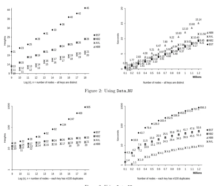
Data – Random and Unique: Data RU The set,Data RU, contains 1.2 million distinct records with uniform distribution in random order. Our first experiment is to construct BST, AVL, NB2, and NB8trees usingData RU. The results are compared in Figure 2. Using the heights of BST as the standard, we observe that NB2improves about 35%, while the AVL tree improves about 50%.4 Increasing the value of balance degreekto 4 (not shown in Figure 2 for clarity), the heights will be close to the AVL tree’s. Whenk= 8, the heights are slightly better than the AVL tree’s and very close to optimums. Regarding the computational cost, our results show that NB2 and BST on Data RUare about the same, which is about 20% faster than the AVL tree. However, NB8 runs slower but not by too far and NB8are trees with heights almost optimal.
21 23 25 28 31 33 36 40 42 13 15 18 19 21 22 24 25 26 11 12 13 14 16 17 18 19 20 21 45 28 10 11 12 13 15 16 17 18 19 20 9 14 19 24 29 34 39 44 9 10 11 12 13 14 15 16 17 18 Log (n), n = number of nodes -- all keys are distinct
H e ig h ts BST NB2 AVL NB8 0.70 1.77 2.83 4.00 5.21 6.47 7.80 9.22 10.63 12.10 13.60 15.14 7.98 9.03 10.40 11.56 0.46 1.10 1.82 2.55 3.32 4.15 5.05 5.88 6.75 7.63 8.56 9.45 0.57 1.30 2.15 3.06 3.99 4.97 5.92 6.94 0.41 0.98 1.612.35 3.10 3.91 4.68 5.49 6.37 7.26 8.17 9.21 0 5 1 0 1 5 2 0 0.1 0.2 0.3 0.4 0.5 0.6 0.7 0.8 0.9 1 1.1 1.2 Millions
Number of nodes -- all keys are distinct
S e c o n d s NB8 AVL NB2 BST
Figure 2: UsingData RU
18 22 28 36 52 82 134 247 469 905 13 17 19 22 24 26 29 31 33 10 13 14 15 16 17 14 12 18 19 20 11 12 19 20 21 1 1 0 1 0 0 1 0 0 0 9 10 11 12 13 14 15 16 17 18 Log (n), n = number of nodes -- each key has n/100 duplicates
H e ig h ts BST NB2 AVL NB8 4.3 18.8 43.7 79.4 126.0 183.4252.5 336.9453.8 572.4707.2 856.3 11.5 15.9 20.5 25.5 30.8 36.1 41.7 47.6 53.6 19.5 24.3 29.4 34.5 39.9 45.5 51.3 1.9 2.6 3.3 4.1 4.9 5.7 6.6 7.5 8.4 9.3 7.6 4.2 15.1 10.9 7.2 4.0 1.4 1.1 1 1 0 1 0 0 1 0 0 0 0.1 0.2 0.3 0.4 0.5 0.6 0.7 0.8 0.9 1 1.1 1.2 Millions
Number of nodes -- each key has n/100 duplicates
S e c o n d s BST NB2 NB8 AVL
Figure 3: UsingData RD
Data – Random and Duplicate: Data RD In applications, there may be cases that we don’t have enough key space to assign a distinct key to each record. For example, there is no need to distinguish among postal mails that are sent to the same region with the same zip code in a processing center. To reflect this situation, we create another data set, Data RD, with 1.2 million records in which each key has 12,000 duplicates distributed uniformly in the data set. In other words, each key in a set ofn records drawn from Data RDis expected to have n/100 duplicates. Under this situation, BST is totaly out of control (see Figure 3). NBk performs much
better than BST even whenkis as small as 2. While NBk can be constructed much faster than BST (the time
needed is only about 6% of the time needed for constructing BST), it is about 5 times slower than constructing the AVL tree.
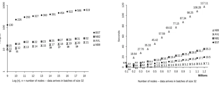
Data – Sorted in Batches: Data SB It may not be realistic to assume data to be inserted are distributed uniformly and completely random. There is another common situation in real applications, in which data may arrive in batches. Each batch may arrive randomly but each contains some sorted records. Instead of using batches, we are asked to insert each record as an independent node into a binary search tree. One can image that a postal mail procession center receives mails batch by batch, and each batch comes from a zip code region. Moreover, the mails in each batch are sorted by their regional office. To simulate this situation, we generate a data set namedData SBalso containing 1.2 million records. The size of each batch is fixed to 32. To generate a batch, we first generate a record (with 3 keys) as before and then set the third key to 0. Then, generate another 31 records with the first two keys identical to the first record’s and the third keys set to 1, 2,. . ., 31 in order.
130 226 293 327 360 391 454 522 586 619 15 18 22 22 23 25 27 28 31 32 11 12 13 14 15 18 19 20 21 17 10 11 16 17 18 19 1 1 0 1 0 0 1 0 0 0 9 10 11 12 13 14 15 16 17 18 Log (n), n = number of nodes -- data arrives in batches of size 32
H e ig h ts BST NB2 AVL NB8 18.64 27.70 35.33 45.42 57.59 69.02 77.15 87.34 98.25 108.28 117.11 2.6 3.3 3.9 4.5 5.2 5.8 6.5 7.1 13.9 16.7 19.4 22.2 25.1 28.5 31.7 35.3 7.3 9.0 10.7 12.4 14.2 15.9 17.7 19.5 5.582.3 1.2 0.6 5.5 2.6 0.9 8.3 4.2 1.5 11.1 5.7 2.0 0 2 0 4 0 6 0 8 0 1 0 0 1 2 0 0.1 0.2 0.3 0.4 0.5 0.6 0.7 0.8 0.9 1 1.1 1.2 Millions
Number of nodes -- data arrives in batches of size 32
S e c o n d s NB8 AVL NB2 BST
Figure 4: UsingData SB
Figure 4 shows the results. The speed of constructing BST is acceptable but the heights of the resulting trees are out of control. As we expect, NB2 and NB8can perfectly manage the heights, but their constructing times become slow; only NB2 runs within an acceptable range.
4
Conclusion
Based on our experimental results, NBk can be used under some controlled conditions (like data in Data RU
and Data RD), but in general it is no replacement for those classic balancing techniques such as AVL trees.
Our main purpose of introducing NBk is pedagogical. Compared to any other balancing methods found in the
literature, our node-balanced binary search tree is the easiest one. Thus, we believe that our approach is an immediate step to move after students have learned binary search trees, and we also believe that our approach should be considered as a missing intermediate step towards a mature yet complicate technique for balancing binary search trees.
References
[1] G. M. Barnes, J. Noga, P. D. Smith, and J. Wiegley. Experiments with balanced-sample binary trees.
SIGCSE 2005, 37(1):166–170, March 2005.
[2] T. H. Cormen, C. E. Leiserson, and R. L. Rivest. Introduction to Algorithms. The MIT Press, Cambridge, Massachusetts, 1989.
[3] L. Devroye and B. Reed. On the variance of the height of random binary search trees. SIAM J. Comput., 24(60):1157–1162, 1995.
[4] M. Drmota. An analytic approach to the height of binary search trees. Algorithmica, 29(1):89–119, 2001. [5] A. Drozdek. Data Structures and Algorithms in C++. Thomson Course Technology, third edition, 2005. [6] E. Horowitz and S. Sahni. Fundamentals of Data Structures in Pascal. Computer Science Press, Inc., 1984. [7] B. Manthey and R. Reischuk. Smoothed analysis of the height of binary search trees. Electronic Colloquium
on Computational complexity, (60), 2005.
[8] C. Okasaki. Alternatives to two classic data structures. SIGCSE 2005, 37(1):162–165, March 2005. [9] M. A. Weiss. Data Structures and Problems Solving Using JAVA. Addison Wesley, third edition, 2006. [10] N. Wirth. Algorithm + Data Structures = Programs. Prentice-Hall, Inc, 1976.