International Consumption Patterns: Evidence from the 1996 International Comparison Project

International Consumption Patterns: Evidence from the 1996 International Comparison Project

James Seale, Jr., University of Florida (352) 392-2297 ext. 414

(352) 392-3646 fax

[email protected]

Anita Regmi, MTED/ERS1 (202) 694-5161 (202) 694-5795

[email protected]

Paper presented at the Sixth Annual Conference On Global Economic Analysis June 12-14, Scheveningen, The Netherlands

1 _{James Seale is Professor, University of Florida, and Anita Regmi is Senior Economist, Economic Research}

Service, USDA. The authors wish to express their deep appreciation to Yonas Biru and Yuri Dikhanov, World Bank, for making the data available. Without their assistance, the study would not be possible. The authors also wish to express thanks to Tom Hertel (U of Purdue), Jeffrey Reimer (U of Wisconsin) and Terry Roe (U of Minnesota) for their helpful review comments on earlier versions of the paper.

International Consumption Patterns: Evidence from the 1996 International Comparison Project

James Seale, Jr. and Anita Regmi

Key words: consumption, cross-country demand, elasticity, heteroskedasticity, maximum likelihood.

Abstract

The Florida model, a modified Working’s model that incorporates price terms, is fit to the 1996 International Comparison Project’s data for nine broad categories of goods across 114 countries. The country data exhibit group heteroskedasticity, and a maximum likelihood procedure that corrects for group heteroskedasticity is developed and used to estimate the model. Outliers are identified with information inaccuracy measures, and Strobel measures of goodness-of-fit are calculated. Results suggest that low-, middle-, and high-income countries have distinct income and price responses; low-income countries are more responsive to income and price changes than high-income countries. Additionally, the conditional demand for eight food subcategories is fit to the data and results are linked to the aggregate level results to calculate conditional and unconditional expenditure elasticities for these goods.

James Seale is Professor, University of Florida, and Anita Regmi is Senior Economist, Economic Research Service, USDA. The authors wish to express their deep appreciation to Yonas Biru and Yuri Dikhanov, World Bank, for making the data available. Without their assistance, the study would not be possible. The authors also wish to express thanks to Tom Hertel (U of Purdue), Jeffrey Reimer (U of Wisconsin) and Terry Roe (U of Minnesota) for their helpful review comments on earlier versions of the paper.

International Consumption Patterns: Evidence from the 1996 International Comparison Project

James Seale, Jr. and Anita Regmi

Introduction

A two-stage demand model (the Florida Model) is fit to the 1996 International

Comparison Project (ICP) data for nine broad categories (food, beverage and tobacco; clothing and footwear; education; gross rent, fuel and power; house furnishings and operations; medical care; recreation; transport and communications; and other items) and eight food sub-categories (cereals, meat, fish, dairy products, oils and fats, fruits and vegetables, beverage and tobacco, and other food) of goods.2 The data contain consumption information for 114 low-, middle-, and high-income countries and include some Former Soviet Union countries. We divide the

countries into three groupings: countries that were included in Phases II, III, and IV of the ICP; countries added to the ICP sample in Phase IV; and those added in the 1996 ICP data. The covariances of these three groups exhibit heteroskedasticity, and a maximum-likelihood procedure is developed and implemented to correct for it.3

Information inaccuracy measures derived from information theory are used to identify outliers.4 Of the 115 countries in the 1996 ICP data, one (Herzegovina) is omitted due to lack of population data while 23 others are identified as outliers and omitted from the final data set of 91 countries. Heteroskedastic-corrected parameter estimates are obtained and used to calculate country-specific income and price elasticities of demand for the nine broad categories and income elasticities for the eight food sub-categories of goods.

2 _{The model, developed by Theil, Chung and Seale (1989), was originally named the Working PI (Preference}

Independence) model but was renamed the Florida model by Seale, Walker and Kim (1991). In later writings, Theil (1996) also referred to it as the Florida model.

3 _{Theil, Chung and Seale (1989), and Seale, Walker and Kim (1991) also found group heteroskedastic covariances}

This paper first describes the 1996 ICP data used in the demand analysis. This is

followed by a brief discussion of the Working’s (1943) model and the Florida model. A section on information inaccuracy measures and their use in identifying outliers follows the discussion. Parameter estimates are presented and compared to those of Theil, Chung and Seale (1989). Finally, the estimated income and price elasticities for the aggregate model and the estimated expenditure elasticities for the disaggregate food model are briefly discussed.

International Comparison Project (ICP) Data

The International Comparison Project (ICP) was originally initiated by researchers at the University of Pennsylvania (Kravis et al., 1975) and is currently coordinated by the Technical Assistance and Statistics Division of the World Bank. Over the years, the number of countries included in the ICP data has increased; there were 10 countries in the 1970 Phase I (Kravis et al., 1975), 16 countries in the 1970 Phase II (Kravis, Heston and Summers, 1978), 34 countries in the 1975 Phase III (Kravis, Heston and Summers, 1982), 60 countries in the 1980 Phase IV (United Nations, 1986-87), and 115 countries in 1996 (table 1).5 The 1996 data introduce an additional 65 countries not included in Phases II through IV, but 10 previously included countries are not represented in the data for a total of 60 +65 –10 = 115 countries.

To conduct cross-country analysis, real consumption expenditures in different currencies must be expressed in terms of a base-country currency comparable across countries. One solution is to convert expenditures into a single currency by using exchange rates. However, exchange rates do not account for the fact that services are cheaper in low-income countries.

4 _{Theil, Chung and Seale (1989) used this method to identify outliers in earlier Phases of the ICP.} 5 _{The 1970 Phase II supercedes the 1970 Phase I.}

Therefore, exchange rates tend to overstate the poverty of poorer countries. To obtain more accurate estimates for individual countries, the Geary-Khamis method of aggregation can be utilized to obtain prices and volumes in terms of purchasing power parities (PPPs) relative to a base country (World Bank, 1993). These values allow comparisons at various levels of

aggregation for all countries included in the analysis. The procedure yields volumes in the form of expenditures expressed in “international dollars.” Such volumes are additive across

expenditure categories, while prices can be obtained by dividing expenditures in national currency by those in international dollars. Because prices remain in national currency denominations, any model fit to the data must explicitly take this into account.6

Working’s Model

In its general form, Working’s (1943) model states that, for n goods, i = 1,…,n, log

i i i

w =α β+ E +ε_i (1)

where w_i P Ei i E

= equals the budget share for good i, represent the price of and

expenditure on good i, respectively,

and

i

P Ei

E

1 n

i i

E=

∑

and the α_i andβ_iare parameters to be estimated. Since the budget shares across all consumption groups sum to 1, the α’s and β’s are subject to the adding-up conditions,

∑

α and

∑

= = n i i 1 0 β

6 _{See Theil, Chung and Seale (1989) Appendix A, for a discussion of the Geary-Khamis methodology and how to}

estimate PPPs based upon it. Data related problems encountered and the methods used to resolve the problems are described in Seale, Regmi and Bernstein, forthcoming 2003.

The marginal budget share, θi, is not constant but varies by affluence, and it exceeds the budget shares by βi ;

(

)

i i i

i E w

dE

dE _{α β β}

θ = = + 1+log = + . (3)

Accordingly, when income changes, wichanges as does the marginal share.

Florida Model

The Florida model, developed by Theil, Chung and Seale (1989), is derived from Working’s (1943) model using the differential approach (Theil, 1980) and is developed

specifically to analyze the ICP data. The simple model developed by Working to estimate U.S. household demand for broad categories of goods assumes that all households face the same price vector. Theil, Chung and Seale (1989) incorporate price terms into Working’s model using the differential approach. They note that equation (1) predicts the budget share when all countries face an identical price vector while the observed budget share is based on equation (1) plus the fact that countries face different price vectors. Thus, they derive the price terms of the Florida model by first adding dw to both sides of equation (1) where is the observed budget share and is the predicted budget share from equation (1). Next, total differentiation yields the Florida model. Specifically, the Florida model can be written in terms of good i and country c as follows,

ˆ

i =wi−wi wi

i

wˆ

=

ic

w LINEAR + QUADRATIC + CUBIC +ε_ic, (4)

LINEAR = Real-income term,

QUADRATIC = Pure price term, =

(

)

(

)

∑

j j j c

i ic c i i P P q P P

q log ₁α β log

β

α , and (4.b)

CUBIC = Substitution term,

=

(

)

(

)

∑

j j j c

i ic c i i P P q P P

q* log _{1α β} * log

β α

φ , (4.c)

where q_cis the naturallogarithm of (real per capita income (expenditure) in country c),

(1+ c Q * _), c c

q ₌ q P_i is the geometric mean price of good i across all countries and φ represents the income flexibility (the inverse of the income elasticity of the marginal utility of income).

The linear term in the model, equation (4.a), represents the effect of a change in real income (i.e., the volume of total expenditure) on the budget share. Since the quadratic and cubic terms vanish at geometric mean prices, the linear term is also the budget share at geometric mean prices. The quadratic term, equation (4.b), (quadratic because it contains products of the α’s and the β’s) is the pure-price term that shows how an increase in price results in a higher budget share on good i, even if the volume of total expenditure stays the same. The cubic term, equation (4.c), (cubic because it involves φ as well as the α’s and β’s) is a substitution term reflecting how higher prices may cause lower budget shares for good i due to substitution away from good i

towards other (now) relatively cheaper goods. This model assumes preference independence among the consumption categories and is also known as the Florida PI model. Given the

assumption of preference independence the model is better suited for analysis of broad consumption categories as used in our analysis.

The Florida-Slutsky model, which assumes weak separability, is used to estimate the second stage of the model, the food subcategories. Similar to the PI model, the Florida-Slutsky model has three components; a linear real-income term; a quadratic pure-price term; and a linear substitution term replacing the cubic term in the former model, that is,

(5.a)

c i i

ic q

w =

α

β

+

(

)

(

)

∑

log α β

β

α _(5.b)

+ log

1        

∑

π _(5.c)

Income and price elasticities estimated from the Florida-Slutsky model are conditional on given food expenditures. The unconditional demand elasticities can then be obtained using the

parameters estimated in the first step of the analysis. For example, the unconditional income elasticity (ηUic) is simply the conditional elasticity (ηCic) multiplied by the income elasticity of

demand for food as a group(ηFc ) obtained from the Florida-PI model, or

ηU

Information Inaccuracy Measures and Outliers

The earlier phases of the ICP data contained several outliers, especially African countries, where the data are quite unreliable (Theil, Chung and Seale, 1989).7 Similarly, scatter plots of the 1996 data also revealed some outliers. To identify outliers, we follow the strategy of Theil, Chung and Seale (1989) and calculate information inaccuracy measures from statistical

information theory. Specifically, the information inaccuracy measure is

1 log

ˆ

w

w

I

∑

_w

where wic is the observed budget share of good i in country c, and is the fitted budget share of good i in country c based on equation (4). When the model fits perfectly, , and the value of I

wˆic

ic wˆ

i

ic ic=w ∀ wˆ

cis zero. The value is positive when, for some i in c, −wic is non-zero. Let the differenceequal the residual, eic. A Taylor expansion shows that when these residuals are sufficiently small, 2 1 1 2 n ic c i _ic

e

I

∑

_w

Following Theil, Chung and Seale (1989), countries with Ic >.10 (at two decimal places) are declared to be outliers. Of the original 114 countries, 23 countries are identified as outliers and omitted from the data set. Of these 23 countries, seven (Cote d’Ivoire, Egypt, Madagascar, Malawi, Nigeria, and Tanzania) are from Africa, three (Bahamas, Ecuador, and Paraguay) are from America, one (Albania) is from Europe, six (Armenia, Azerbaijan, Georgia, Mongolia,

7 _{This is true even for population data. Seale and Theil (1986) note that, according to The Economist, July 20,}

1985:30, the 1984 population estimate of the Ethiopian government based on prior censuses differed from the actual mid-1984 census by no less than nine million out of a population of 43 million.

Tajikistan and Turkmenistan) are from Central-Asian-transition countries, and six others (Bahrain, Hong Kong, Iran, Philippines, Sri Lanka, and Yemen) are also from Asia.

It is interesting to note that whether or not a country’s data are outliers appears to be related to when the country first appears in the ICP study. For example, there are only three outliers among the countries that are in the first three ICP phases. Of the 33 countries introduced in Phase IV, eight are outliers, five of which are low-income African countries. Of the 60

countries introduced in 1996, 12 are outliers, seven of which are transitional economies, four of which are Middle Eastern, and the last of which is the Bahamas.

Parameter Estimates

All parameters of the Florida-PI and the Florida-Slutsky model were estimated by maximum likelihood (ML) using the scoring method (Harvey, 1990, pp. 133-135) and the GAUSS software8. Theil, Chung and Seale (1989) note that the average information inaccuracy measures vary substantially between countries present both in Phases III and IV and those newly added in Phase IV. Further, they divide the Phase IV data into two groups, countries in either Phases II or III and those that are not in either. Fitting the Florida model to the group data individually, they find that the group covariance matrices are not equal; the covariance matrix of the group of newly added countries is almost twice as large as that of the group of countries in Phases II or III. Given this difference, they infer that the covariance matrices of these two groups are heteroskedastic.

8 _{For the development and a discussion of the maximum-likelihood procedure used in estimating the model and}

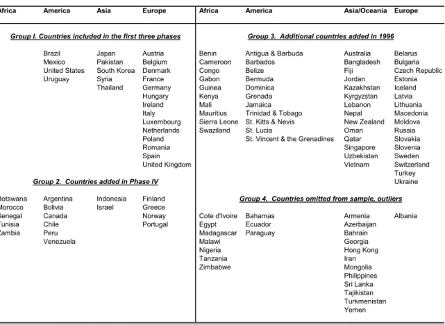
We extend this approach and allow for heteroskedasticity among the three separate groups of countries: Group 1, those included in Theil, Chung and Seale’s (1989) estimation from the first three phases of the ICP; Group 2, those added in Phase IV; and Group 3, those countries first appearing in the 1996 ICP data (and not in the first four phases). Group 1 has 23 countries, Group 2 has 17 countries, and Group 3 has 51 countries (table 2). We normalize Kg = 1 for

Group 1 countries and estimate two heteroskedastic parameters. Income is normalized so that the per capita real income of the United States equals one, and all other country per capita real incomes are relative to that of the United States.

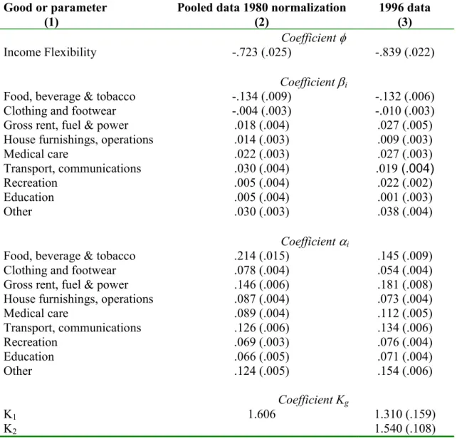
The parameters and their associated asymptotic standard errors are estimated with the heteroskedastic-corrected ML procedure for the 91 countries, and the results are presented in tables 3 and 4. For comparative purposes, parameter estimates obtained by Theil, Chung and Seale (1989, table 5-4, column (3), p. 105) for their 1980 normalized and pooled data are

reported in column (2) of table 3. Our estimated income flexibility, -.839, is negative, consistent with expectations, and is somewhat more negative than the value, -.723, obtained by Theil, Chung, and Seale (1989). The estimated two Kgs exceed 1 confirming the presence of

heteroskedasticity.

As indicated by the negativeβs only food, beverage and tobacco, and clothing and footwear are necessities; all other consumption categories except education are luxuries. The category education has a near zero βiand hence has near-unitary income elasticity. The β parameter for food, beverages and tobacco is by far the largest β in absolute value. Its estimate of –.132 (with an asymptotic standard error of .006) is comparable to the value, -.134, obtained by Theil, Chung and Seale (1989, table 5-4, p. 105) for the 1980 normalization of their extended

and pooled data.9 This parameter estimate retains the property of the strong version of Engel’s law: when income doubles, the budget share of food declines by approximately 0.1 (Theil, Chung and Seale, 1989, p. 44, 139). The αs from this study and those of Theil, Chung and Seale (1989) are not comparable since their data are normalized on 1980 geometric-mean prices while the current data are in 1996 prices.

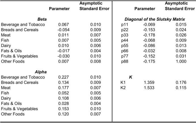
Table 4 presents the estimated parameters for the second-stage model, the food sub-groups. Similar to the aggregate model, the estimated two Kgs exceed 1 confirming the presence

of heteroskedasticity. As indicated by the negative sign ofβs, bread and cereals, fats and oils and, fruits and vegetables are (conditionally) inelastic food items while the remaining 5 are conditionally elastic items.10 The negative β for fruits and vegetables can be explained by the fact that the data for this food sub-category also include expenditures on roots and tubers, a staple among poor consumers. The piis in the table present the compensated own-price effects, the diagonal of the Slutsky matrix, used in calculating the own-price elasticities.

Income and Price Sensitivity

The most prominent measures of income and price sensitivities for a good are income and own-price elasticities. These measures are not constant but should vary with different levels of affluence. For example, the income elasticity of demand for a necessity such as food, beverages and tobacco should be larger for a low-income county than for a high-income country.

9 _{The estimate of -.134 for food, beverages and tobacco is obtained by simply adding the parameter estimate of food,}

-.135, to that of beverages and tobacco, .001.

10 _{Remember the parameter estimates are conditional on total per capita food expenditures, not total per capita}

price elasticities of demand should also be larger in absolute value for low-income countries than for high-income ones (Timmer, 1981).

The income elasticity of demand for the Florida PI and the Florida Slutsky models are given by the ratio of the marginal share to the budget share,

(log ) =1+ (log )

i i i

i

i i

dE E d E B

w dE E d E w

i

θ

= = . (8)

From equation (8), we note that a luxury good (with income elasticity greater than 1) is

associated with a positive βi, while the βi is negative for a necessity (income elasticity less than

1). If βi equals zero, the good has unitary elasticity.

The Aggregate Model

The country-specific income-elasticity values represent the estimated percent change in demand for a particular good if total income changes by one percent. Table 5 presents the average budget shares and income elasticities for the 9 aggregate consumption categories calculated at 1996 geometric mean prices for the 3 groups of countries; low-, middle-, and high-income countries. In this analysis, low-high-income countries have per capita high-income levels below 16 percent of the U.S. level, middle-income countries between 16 and 46 percent of the U.S. level, and high-income countries greater than 46 percent of the U.S. level. Of the 91 countries, 22 are low-income countries, 40 are middle-income countries, and the remaining 29 are high-income countries.

The income elasticity of demand for food, beverages and tobacco varies greatly among countries and is highest among low-income countries; it varies from .78 for Zambia to .66 for Thailand. It ranges between .65 to .47 for middle-income countries and from .45 to .09 for

high-income countries. Its average high-income elasticity in the low-high-income group of countries is .72, and it is over twice the size of the average, .32, of high-income countries. For high-income

countries, the income elasticity of demand for food, beverages and tobacco gradually decreases from .45 for the Czech Republic, with an income level 48 percent that of the United States, to .24 for Denmark whose income level is 80 percent that of the United States. Thereafter, the

elasticity measure decreases rapidly to .11 for Luxembourg and .09 for the United States. The income elasticity of demand for education is statistically unitary with a point estimate of 1.01 for all countries. Elasticities for all other categories are higher for less affluent countries and span a wide range. Recreation is by far the most luxurious good with an income elasticity of demand ranging from 6.35 for Zambia to 1.28 for the United States. The goods, medical care and other items, are also luxuries, and their income elasticities vary from 2.18 and 2.38 for Zambia respectively, to 1.24 and 1.25 for the United States, respectively.

Three types of own-price elasticities of demand for a good can be calculated from the parameter estimates of the Florida model. The first of these, the Frisch-deflated own-price elasticity of good i, is the own-price elasticity when own-price changes and income is

compensated to keep the marginal utility of income constant. In the case of the Florida model, the Frisch own-price elasticity is

ic i ic

w w

F =φ +β (9)

where w_ic is calculated from equation (1) with the error term suppressed, and φ and βi are estimated parameters of the Florida model.11

The Slutsky (compensated) own-price elasticity measures the change in demand for good i when the price of i changes while real income remains unchanged. Since real income is

constant, this elasticity is also referred to as the ‘pure substitution effect.’ It is calculated from the following,

(

)(

)

₍

i ic ic

i ic i

ic _{F w}

w w w

S =φ +β 1− −β = 1− −β

)

The Cournot (uncompensated) own-price elasticity refers to the situation when own-price changes while nominal income remains constant but real income changes. This measure

includes both the pure substitution effect and the income effect due to a price change. It is therefore greater in absolute value than the Slutsky own-price elasticity and is calculated from

(

)(

_{) (}

₎

₍

i ic i

ic ic

i ic i

ic _{w S w}

w w w

C =φ +β 1− −β − +β = − +β

)

These three types of own-price elasticities are calculated for all nine goods for the 91 countries and the average values for the 3 groups of countries are presented in table 6. The elasticity measures perform in accordance with Timmer’s proposition: own-price elasticities of demand are larger in absolute values for low-income countries than for high-income ones. The values of the Cournot and Frisch own-price elasticities decline monotonically in absolute value when traveling from poor to rich countries. For example, the average Cournot own-price elasticity for food ranges from -.74 for low-income, -.60 for middle-income and -.32 for high-income

countries. The Frisch own-price elasticity for food are -.61, -.50 and -.27 for the 3 groups of countries, respectively.

The Slutsky ownprice elasticity of demand for food, beverages, and tobacco begins at .35 for Zambia, increases (absolutely) to .41 for Turkey, and declines thereafter (absolutely) to

-.07 for the United States. Therefore, the average values for country groups are -.39 for low-income, -.40 for middle-income and -.25 for high-income countries.

The Cournot elasticity values are all larger than the corresponding Slutsky elasticities, and the Frisch values are between the corresponding Cournot and Slutsky ones. Recreation, and medical care are the only goods that have Slutsky own-price elasticity measures greater than unity in absolute terms. For the lowest-income countries, Slutsky measures are less than –1.0 but eventually become greater than –1.0 for some middle- and high-income countries. For Zambia, the Slutsky own-price elasticities of demand for recreation, medical care, and other items are – 5.19, -1.74, and –1.87, respectively; for the United States, they are -.97, -.89, and -.86,

respectively.

Dis-aggregate food expenditure elasticities

The expenditure elasticities calculated using the Florida-Slutsky model are conditional on a given food budget. In other words, the conditional expenditure elasticity measures the

percentage change in demand for a 1-percent change in food budget. However, the conditional elasticities can be converted to unconditional elasticities using the parameters estimated from the Florida-PI model in the first stage. The unconditional elasticities measure percentage change in demand from a 1-percent change in overall income (expenditures).

With βi> 0 for 5 of the 8 food subcategories, the estimated conditional income elasticities are greater than 1 for these 5 food groups, indicating these to be (conditional) elastic food items. However, using equation (6) the conditional income elasticity is converted to unconditional income elasticity. The estimated income (expenditure) elasticities presented in figure 1 are all less than 1, excepting for beverage and tobacco in low-income countries. This is consistent with

conventional theory that food is a necessity and not a luxury item in household expenditures. Given the relatively low food budget share of beverage and tobacco in many low-income countries, this category can be considered a luxury item among consumers in some poorer countries.

Similar to the estimated income elasticity for aggregate consumption categories, the income elasticities for food sub-categories are the largest for the poorest country (Zambia) and decline in magnitude with affluence, with the smallest elasticities for the United States. For example, the average income elasticity for cereals is 0.55 for low-income countries, 0.41 for middle-income countries, and 0.20 for high-income countries (table 7). Across each country, staple food items (with negative βi) have smaller elasticities than the more conditionally elastic food items such as beverages, meat and dairy. For example, the individual country income elasticity for cereals ranges from .62 in Zambia, to .55 in Thailand, .31 in Korea and .05 in the United States. In contrast, the elasticity for beverages and tobacco are higher across all countries, ranging from 1.48 in Zambia, 1.18 in Thailand, .63 in Korea and .12 in the United States.

Conclusions

Income and own-price elasticities of demand for the nine aggregate categories and expenditure elasticities for the eight disaggregate food subcategories of goods vary significantly among countries of differing levels of affluence. This is particularly true of food, beverages and tobacco; its income elasticity of demand for the poorest country, Zambia, is almost ten times greater than that for the richest country, the United States. The U.S. Cournot (Slutsky)

own-price elasticity of demand for this consumption category is nine (seven) times larger in absolute value for Zambia than for the United States.

The same patterns in the elasticity measures are found for certain luxurious goods: gross rent, fuel and power; house furnishings and operations; medical care; recreation; and other items. The demand for these goods is much more responsive to income changes in low-income than in high-income countries. Interestingly, the own-price elasticities of demand for several goods are larger than unity for low-income countries but less than unity for high-income countries. This is the case for all three-types of own-price elasticities for the following goods: medical care;

recreation; and other items. It is also the case for the Frisch and Cournot own-price elasticities of demand for gross rent, fuel and power, and for transportation and communications.

Low-income countries are also more responsive to income and food price changes, and therefore, make larger adjustments to their overall food consumption pattern with changes in incomes and prices. However, our study illustrates that adjustments to price and income changes are not made uniformly across all food categories. Staple food consumption changes the least, while greater changes are made to higher-value food items such as dairy and meat.

This paper accomplishes two major goals. The first is presenting a two-stage cross-country demand model that enables estimating unconditional income and price elasticities for disaggregate consumption sub-groups, while the second is providing income and price

elasticities across 91 countries for nine aggregate consumption categories and eight food subcategories. While previous research works have presented multi-stage demand estimation models, there have been no empirical works conducted across as many countries and

References

Barten, A.P., 1969, “Maximum Likelihood Estimation of a Complete System of Demand Equation,” European Economic Review 1, 7-73.

Harvey, A., 1990, The Econometric Analysis of Time Series, 2nd Edition (MIT Press, Cambridge, MA).

Kravis, I.B, A.W. Heston, and R. Summers, 1978, International Comparisons of Real Product and Purchasing Power, The Johns Hopkins University Press, Baltimore, MD.

Kravis, I.B., A.W. Heston, and R. Summers, 1982, World Product and Income: International Comparisons of Real Gross Products, The Johns Hopkins University Press, Baltimore, MD.

Kravis, I.B., F. Kennessey, A.W. Heston, and R. Summers, 1975, A System of International

Comparisons of Gross Product and Purchasing Power, The Johns Hopkins University

Press, Baltimore, MD.

Seale, J.L., Jr., and H. Theil, 1986, “Working’s Model for Food in the Four Phases of the International Comparison Project,” Economics Letters 22, 103-104.

Seale, J.L., Jr., W.W. Walker, and I.M. Kim, 1991, “The Demand for Energy: Cross Country Evidence Using the Florida Model,” Energy Economics 13, 33-40.

Seale, J.L., Jr., A. Regmi, and J. Bernstein, Forthcoming 2003, International Evidence on Food Consumption Patterns, Technical Bulletin, ERS-USDA, Washington D.C.

Strobel, D., 1982, “Determining Outliers in Multivariate Surveys by Decomposition of a

Measure of Information,” Proceedings of the American Statistical Association, Business and Economics Section, 31-35, American Statistical Association, Washington, D.C.

Theil, H., 1980, The System-Wide Approach to Microeconomics, University of Chicago Press, Chicago, IL.

Theil, H., 1996, Studies in Global Econometrics, Kluwer Academic Press, Boston, MA. Theil H., C. F. Chung, and J.L. Seale, Jr., 1989, International Evidence on Consumption

Patterns, JAI Press, Inc., Greenwich, CT.

Timmer, C.P., 1981, “Is There Curvature in the Slutsky Matrix?” Review of Economics and Statistics 63, 395-402.

United Nations, 1986-87, World Comparisons of Purchasing Power and Real Product for 1980: Phase IV of the International Comparison Project, Two Parts, United Nations

Publication, New York.

Working, H., 1943, “Statistical Laws of Family Expenditure,” Journal of the American Statistical Association, 38, 43-56.

World Bank, 2001, World Development Indicators, Washington D.C.

World Bank, 1993, Purchasing Power of Currencies: Comparing National Incomes Using ICP Data, Socio-Economic Data Division, International Economics Department,

Table 1. Countries Represented in the International Comparison Project

Africa America Asia Europe Africa America Asia/Oceania Europe

Countries represented in Phase I Additional countries added in 1996

Kenya Colombia India France Benin Antigua & Barbuda Armenia Albania United States Japan Germany Congo Bahamas Australia Belarus Hungary Egypt Barbados Azerbaijan Bulgaria Italy Gabon Belize Bahrain Czech Republic United Kingdom Guinea Bermuda Bangladesh Estonia

Mauritius Dominica Fiji Herzegovina

Countries added in Phase II Sierra Leone Grenada Georgia Hungary

Swaziland Trinidad & Tobago Jordan Iceland Iran Belgium St. Kitts & Nevis Kazakhstan Latvia South Korea Netherlands St. Lucia Kyrgyzstan Lithuania Malaysia St. Vincent & the Grenadines Lebanon Macedonia Philippines Mongolia Moldova

Nepal Russia

Countries added in Phase III New Zealand Slovakia

Oman Slovenia Malawi Brazil Pakistan Austria Qatar Sweden Zambia Jamaica Sri Lanka Denmark Singapore Switzerland

Mexico Syria Ireland Tajikistan Turkey Uruguay Thailand Luxembourg Turkmenistan Ukraine

Poland Uzbekistan

Romania Vietnam

Spain Yemen

Yugoslavia

Countries in previous phases but excluded in 1996 Countries added in Phase IV

Ethiopia Colombia India Yugoslavia Botswana Argentina Hong Kong Finland Costa Rica Malaysia

Cameroon Bolivia Indonesia Greece Dominican Republic Ethiopia Canada Israel Norway El Salvador Cote d'Ivoire Chile Portugal Guatemala Madagascar Costa Rica Honduras Mali Dominican Rep. Panama Morocco Ecuador

Nigeria El Salvador Countries excluded in Phase IV but included in 1996

Senegal Guatemala

Tanzania Honduras Jamaica Iran Romania

Tunisia Panama Mexico Syria

Zimbabwe Paraguay Thailand

Peru Venezuela

Countries excluded in Phase IV

Jamaica Iran Romania Mexico Malaysia

Syria Thailand

Table 2. Classification of Countries for Correction for Heteroskedasticity

Africa America Asia Europe Africa America Asia/Oceania Europe Group I. Countries included in the first three phases Group 3. Additional countries added in 1996

Brazil Japan Austria Benin Antigua & Barbuda Australia Belarus Mexico Pakistan Belgium Cameroon Barbados Bangladesh Bulgaria United States South Korea Denmark Congo Belize Fiji Czech Republic Uruguay Syria France Gabon Bermuda Jordan Estonia

Thailand Germany Guinea Dominica Kazakhstan Iceland Hungary Kenya Grenada Kyrgyzstan Latvia Ireland Mali Jamaica Lebanon Lithuania Italy Mauritius Trinidad & Tobago Nepal Macedonia Luxembourg Sierra Leone St. Kitts & Nevis New Zealand Moldova Netherlands Swaziland St. Lucia Oman Russia Poland St. Vincent & the Grenadines Qatar Slovakia Romania Singapore Slovenia Spain Uzbekistan Sweden United Kingdom Vietnam Switzerland

Turkey

Group 2. Countries added in Phase IV Ukraine Botswana Argentina Indonesia Finland Group 4. Countries omitted from sample, outliers

Morocco Bolivia Israel Greece

Senegal Canada Norway Cote d'Ivoire Bahamas Armenia Albania Tunisia Chile Portugal Egypt Ecuador Azerbaijan

Zambia Peru Madagascar Paraguay Bahrain

Venezuela Malawi Georgia

Nigeria Hong Kong Tanzania Iran Zimbabwe Mongolia

Philippines Sri Lanka Tajikistan Turkmenistan Yemen

Table 3. Parameters from Maximum Likelihood Estimation Good or parameter

(1)

Pooled data 1980 normalization (2)

1996 data (3)

Coefficient φ

Income Flexibility -.723 (.025) -.839 (.022)

Coefficient βi

Food, beverage & tobacco -.134 (.009) -.132 (.006)

Clothing and footwear -.004 (.003) -.010 (.003)

Gross rent, fuel & power .018 (.004) .027 (.005)

House furnishings, operations .014 (.003) .009 (.003)

Medical care .022 (.003) .027 (.003)

Transport, communications .030 (.004) .019 (.004)

Recreation .005 (.004) .022 (.002)

Education .005 (.004) .001 (.003)

Other .030 (.003) .038 (.004)

Coefficient αi

Food, beverage & tobacco .214 (.015) .145 (.009)

Clothing and footwear .078 (.004) .054 (.004)

Gross rent, fuel & power .146 (.006) .181 (.008)

House furnishings, operations .087 (.004) .073 (.004)

Medical care .089 (.004) .112 (.005)

Transport, communications .126 (.006) .134 (.006)

Recreation .069 (.003) .076 (.004)

Education .066 (.005) .071 (.004)

Other .124 (.005) .154 (.006)

Coefficient Kg

K1 1.606 1.3 (.159)

K2 1.540 (.108)

10

Note: Column 2 figures are from Theil, Chung & Seale, International Evidence on Consumption

Table 4. Maximum likelihood estimates of the food sub-group model, 91 countries in 1996 Parameter

Asymptotic

Standard Error Parameter

Asymptotic Standard Error

Beta Diagonal of the Slutsky Matrix

Beverage and Tobacco 0.067 0.010 p11 -0.069 0.015 Breads and Cereals -0.054 0.009 p22 -0.153 0.024 Meat 0.011 0.007 p33 -0.178 0.026 Fish 0.007 0.005 p44 -0.068 0.009 Dairy 0.010 0.006 p55 -0.086 0.013 Fats & Oils -0.017 0.004 p66 -0.032 0.008 Fruits & Vegetables -0.030 0.010 p77 -0.152 0.031 Other Foods 0.007 0.008 p88 -0.175 1.000

Alpha

Beverage and Tobacco 0.227 0.010 K

Breads and Cereals 0.134 0.009 K1 1.359 0.176

Meat 0.177 0.007 K2 1.533 0.115

Fish 0.052 0.005

Dairy 0.108 0.006

Fats & Oils 0.028 0.004 Fruits & Vegetables 0.153 0.010 Other Foods 0.120 0.007

Table 5: Average Budget Shares and Income Elasticities of Aggregate Consumption Categories by Income Groupings

Consumption Budget Shares Income Elasticity

Categories Low Income Middle Income High Income Low Income Middle Income High Income <16% of U.S. 16-46% of U.S. >46% of U.S. <16% of U.S. 16-46% of U.S. >46% of U.S.

Food, beverage & tobacco 0.30 0.27 0.18 0.72 0.59 0.32

Clothing & footwear 0.05 0.06 0.05 0.88 0.85 0.83

Education 0.11 0.12 0.07 1.01 1.01 1.01

Gross rent, fuel & power 0.14 0.18 0.18 1.25 1.19 1.16

House operations 0.07 0.05 0.06 1.17 1.14 1.13

Medical care 0.06 0.09 0.11 1.64 1.36 1.26

Other 0.04 0.07 0.15 1.70 1.38 1.27

Recreation 0.01 0.02 0.07 2.33 1.48 1.32

Transport 0.21 0.14 0.12 1.21 1.17 1.15

Table 6. Average Own-Price Elasticities of Aggregate Consumption Categories by Income Groupings

Consumption Slutsky Cournot Frisch

Categories Low Income Middle Income High Income Low Income Middle Income High Income Low Income Middle Income High Income <16% of U.S. 16-46% of U.S. >46% of U.S. <16% of U.S. 16-46% of U.S. >46% of U.S. <16% of U.S. 16-46% of U.S. >46% of U.S.

Food, beverage & tobacco -0.39 -0.40 -0.25 -0.74 -0.60 -0.32 -0.61 -0.50 -0.27

Clothing & footwear -0.68 -0.68 -0.66 -0.75 -0.73 -0.71 -0.73 -0.72 -0.70

Education -0.79 -0.79 -0.79 -0.86 -0.86 -0.86 -0.85 -0.85 -0.85

Gross rent, fuel & power -0.90 -0.83 -0.78 -1.04 -1.00 -0.98 -1.05 -1.00 -0.97

House operations -0.93 -0.89 -0.87 -0.99 -0.96 -0.95 -0.98 -0.96 -0.94

Medical care -1.28 -1.03 -0.93 -1.35 -1.13 -1.05 -1.38 -1.14 -1.06

Other -1.29 -1.00 -0.88 -1.39 -1.13 -1.06 -1.43 -1.16 -1.07

Recreation -1.88 -1.16 -1.01 -1.92 -1.22 -1.10 -1.96 -1.24 -1.11

Transport -0.91 -0.86 -0.82 -1.02 -0.98 -0.97 -1.02 -0.98 -0.96

Table 7: Average Conditional Budget Shares and Unconditional Income Elasticities of Food Subcategories by Income Groupings

Consumption Budget Shares Income Elasticity

Categories Low Income Middle Income High Income Low Income Middle Income High Income <16% of U.S. 16-46% of U.S. >46% of U.S. <16% of U.S. 16-46% of U.S. >46% of U.S.

Beverage and Tobacco 0.25 0.18 0.12 1.18 0.82 0.42

Breads and Cereals 0.14 0.18 0.18 0.55 0.41 0.20

Meat 0.05 0.04 0.05 0.77 0.63 0.34

Fish 0.08 0.11 0.10 0.84 0.68 0.37

Dairy 0.06 0.04 0.03 0.80 0.65 0.35

Fats & Oils 0.21 0.18 0.15 0.50 0.33 0.13

Fruits & Vegetables 0.11 0.15 0.27 0.61 0.49 0.26

Other Foods 0.10 0.12 0.12 0.77 0.63 0.34

0.000 0.200 0.400 0.600 0.800 1.000 1.200 1.400 1.600 1.800

Zam bia

Pakist an

Syria Swaz

iland Russia Estoni a

Slov enia

New Z ealand

Germ any United

Stat es

Beverage Cereal Meat Fish Dairy Oils Frts&Veg Other