Inducing Herding with Capacity Constraints
∗
Alexei Parakhonyak
†and Nick Vikander
‡August 2018
Abstract
We show that a firm may benefit from restricting capacity so as to trigger herding
behavior from consumers, in situations where such behavior is otherwise unlikely. We
con-sider a setting with social learning, where consumers observe sales from previous cohorts
and update beliefs about product quality before making their purchase. A capacity
con-straint directly limits sales but also makes information coarser for consumers, who react
favorably to a sell-out because they only infer that demand must exceed capacity. Neither
large cohorts nor unbounded private signals guarantee efficient learning, because the firm
acts strategically to influence the consumers’ learning environment.
JEL classifications: D21, D82, D83
Keywords: social learning, informational herding, cascades, capacity
∗This paper has benefited from discussions with Nemanja Antic, Itai Arieli, Vincent Crawford, Ben Golub, Paul Heidhues, Ignacio Monz´on, Steven Morris, David Myatt, Marek Pycia, Gosia Poplawska, Larry Samuelson, Peter Norman Sørensen, Bruno Strulovici, Balazs Szentes, Curtis Taylor, Marta Troya-Martinez, and participants of the Oxford Economic Theory Workshop, Game Theory Society World Congress (Maastricht 2016), EARIE (Lisbon, 2016), Transatlantic Theory Workshop 2016, Lancaster Game Theory Workshop 2016, International Industrial Organization Conference (Boston, 2017), and the Royal Economic Society Annual Conference 2018, as well as audiences in Cardiff, Gothenburg, and Copenhagen.
†University of Oxford, Department of Economics and Lincoln College. E-mail: [email protected]
1
Introduction
This paper shows that firms may want to strategically restrict capacity in order to influence
consumer learning and trigger positive purchase cascades. As is standard in the literature on
social learning (see foundational papers by Banerjee (1992) and Bikhchandani et al. (1992)), each
consumer receives a noisy private signal about product quality, but also infers some information
from observing earlier sales. To illustrate the mechanism at work, consider ten consumers who
visit a firm, where each buys if and only if her signal was good. A consumer who then arrives
and observes initial sales of three may refuse to buy, even if her own signal was good, because she
infers that only three out of the ten others had a good signal. But if the firm, without knowing
product quality, had initially limited capacity to three sales per period, then the consumer
would observe a sell-out, and only infer that there were at least three good signals. That may
well convince the consumer to buy even if her own signal was bad. Thus, in contrast to Sgroi’s
(2002) suggestion, the presence of multiple ‘guinea pigs’ who do not observe others’ choices need
not promote efficient social learning, because the firm uses capacity to manipulate the learning
environment.
An alternative way to avoid ‘pathological outcomes’ where consumers herd on the wrong
action is to have unboundedly informative signals, as proposed by Smith and Sørensen (2000).
Consumers with such signals will effectively ignore public information and their choices can
generally prevent incorrect cascades. Suppose that in our example, one out of ten consumers
per period is perfectly informed about quality and that the firm is unconstrained. If quality is
low, but say seven consumers in period 1 receive good signals, then everyone will buy in period
2 except for the informed consumer. The informed consumer’s choice not to buy will perfectly
reveal that quality is low and lead to zero sales in later periods. However, this same choice would
not reveal any information if the firm had restricted capacity, because the informed consumer
would be effectively pooled with those who were rationed.1 Learning may not occur despite
private signals being unbounded, namely in situations where learning would hurt the firm.
1In the spirit of Smith and Sørensen (2000), we use the word ‘cascade’ to refer to a situation where all
Our focus on sell-outs and rationing fits in with evidence of a variety of products where
demand appears to persistently far outstrip supply. Shortages for ‘Beanie Babies’ were
accom-panied by extremely high demand from 1996 to 1999, before the resale market crashed shortly
thereafter.2 For high-end restaurants, tables at ‘Noma’ in Copenhagen remain notoriously
dif-ficult to come by, and reported waiting times for ‘Damon Baehrel’ or ‘Club 33’ in the United
States range from ten to fourteen years. Music festivals, such as those in Roskilde and Reading,
also often sell out well in advance, year after year, with tickets for Glastonbury 2016 selling out
in just 30 minutes.3 Sell-outs are also common in professional sports, where the Boston Red
Sox enjoyed a sell-out streak which stretched 2003 to 2013.
Formally, we consider a model of social learning where cohorts of consumers arrive
sequen-tially at a seller and observe sales from previous periods. Informed consumers perfectly know
whether product quality is high or low, whereas uninformed consumers receive a private noisy
signal. Consumers in each cohort simultaneously choose whether to buy or take their outside
op-tion and then leave the game. Initially, without knowing its quality, the seller can set a capacity
constraint, where per period sales cannot exceed capacity. This constraint effectively coarsens
the information of consumers, since they cannot observe the extent of any excess demand.
We show that the seller may find it profitable to restrict capacity even though the constraint
directly limits sales in each period. The reason is that sell-outs drive up uninformed consumers’
willingness to pay, and can generate positive purchase cascades where they all want to buy
regardless of their signal. The result is high sales and excess demand in later periods. This
excess demand can actually benefit the seller, if quality is in fact low, by masking the actions
of informed consumers who choose not to buy, thereby allowing the cascade to be maintained.
Indeed, we show that restricting capacity tends to be optimal in situations that a priori seem
grim: when quality is likely low, and signals are quite accurate.
2Debo et al. (2012) argue that scarcity in the case of Beanie Babies was largely due to seller strategic behaviour.
See also: https://nypost.com/2015/02/22/how-the-beanie-baby-craze-was-concocted-then-crashed/, accessed on April 2, 2018.
3See http://www.glastonburyfestivals.co.uk/glastonbury-2016-tickets-sell-out-in-30-minutes/, accessed on
Our paper contributes to the literature on social learning where agents cannot all perfectly
observe each other’s actions. Different work in this literature has assumed that agents can
ob-serve a random sample of earlier actions that is anonymous (Banerjee and Fudenberg (2004),
Smith and Sorensen (2013), Monz´on and Rapp (2014), Monz´on (2017)) or non-anonymous
(Ace-moglu et al. (2011), Lobel and Sadler (2015)), the aggregate total of all past actions (Callander
and H¨orner, 2009), the aggregate total of one particular action (Guarino et al. (2011),
Her-rera and H¨orner (2013)), or only the choice of an agent’s immediate predecessor (C¸ elen and
Kariv, 2004). In all these cases the information structures is exogenous. In our paper, it is
the firm’s strategic choice of information structure that prevents consumers from learning about
low quality, despite our setting having two features that the literature suggests should promote
learning: multiple consumers who do not have access to social information (see Banerjee (1992),
Sgroi (2002), Acemoglu et al. (2011), Smith and Sorensen (2013), Golub and Sadler (2017));
and unbounded private signals (see Smith and Sørensen (2000), Banerjee and Fudenberg (2004),
amongst many others).
Our paper also relates to recent work that considers how an uninformed designer can choose
an information structure for agents in order to influence social learning. Kremer et al. (2014)
and Che and Horner (2015) both consider settings where agents arrive sequentially, and show
that a designer looking to maximize total surplus may prefer an information structure that is
coarse. Coarse information can encourage agents to experiment which can help them learn from
one another. In contrast, we consider a firm looking to maximize profits, and show that it may
choose a coarse information structure in order to limit learning.
There is also a parallel to the literature on Bayesian Persuasion, where a designer conducts
statistical experiments that reveal information about the unknown state to a decision maker
(see Aumann et al. (1995), Kamenica and Gentzkow (2011) and the large literature that has
fol-lowed). Our seller effectively chooses from a restricted set of experiments, each associated with
a particular capacity; and persuasion is costly, since capacity directly limits sales.4 Gentzkow
4The signal structure associated with a capacity constraint in our setting involves upper-tail censoring:
and Kamenica (2014) also consider a restricted experiment space but focus on sender
competi-tion. Gentzkow and Kamenica (2016, 2017) and Mensch (2018) assume a direct cost associated
with each experiment, whereas our implicit cost of capacity arises indirectly through consumer
behavior.5 While these papers consider static settings, others share our focus on dynamics (see
Au (2015), Ely (2017), Renault et al. (2017), Best and Quigley (2017), Bizzotto et al. (2018),
Orlov et al. (2018)). Bizzotto et al. (2018) and Orlov et al. (2018) both assume the decision
maker can learn from multiple sources, but not from the actions of other players. None of these
papers consider limited capacity or social learning.
The literature on how firms can influence consumer learning about product quality has
mainly focused on pricing (Welch (1992), Bose et al. (2006), Bose et al. (2008), Sayedi (2018)),
although some work has considered strategic scarcity.6 Debo et al. (2012) show that a firm
may reduce service speed so that consumers observe longer queues, since long queues suggest
high quality. In Stock and Balachander (2005), a firm can set low inventory, which consumers
then observe and believe that demand (and quality) is high. Both papers assume the firm is
privately informed about quality, and can potentially use this information to mislead consumers.
Moreover, in contrast to our work, scarcity does not hide information from consumers in these
settings, but instead may actually help reveal it.7
We describe our model in section 2, present our analysis in section 3, discuss further results
related to learning in the long run and pricing in section 4, and section 5 then concludes. All
the proofs are presented in the appendix.
Zapechelnyuk (2018) all show that upper-tail censoring can at times be optimal, when experiments directly reveal information about an unknown state.
5These papers also assume that more informative experiments are more costly. The opposite is true in our
setting, as a higher capacity both reveals more information about demand and limits sales to a lesser extent.
6See also Gill and Sgroi (2008) on product testing, Gill and Sgroi (2012) on choice of reviewers, and Aoyagi
(2010), Liu and Schiraldi (2012), and Bhalla (2013) on simultaneous versus sequential product launch.
7Vikander (2018) considers an informed firm that may limit capacity to influence consumer beliefs, but assumes
2
Model
Suppose there is a product or service of unknown quality and two possible states of the world,
Ω ={G, B}. In state G, quality is good and each consumer who buys obtainsuG = 1. In state
B, quality is bad and each consumer who buys obtains uB = 0. A consumer who does not buy
gets reservation utility r ∈(0,1).
The actual state is not known initially to the seller nor to consumers. A priory beliefs of all
players are that P(G) ≡ β and P(B) = 1−β. In each period there are 2n potential buyers,
who are either informed or uninformed. Before making her purchase decision, each informed
consumer receives a signal that reveals the state for sure. Each uninformed consumer receives
a noisy private signal, s ∈ {g, b}, where P(g|G) = P(b|B) ≡ α ∈ (1/2,1). By α < 1, our
signals are boundedly informative. We also assume that a consumer without further information
would follow her signal, i.e. P(G|s =g)> r > P(G|s =b). We model the number of informed
consumers in two ways. In the deterministic setting, we will assume there is a fixed number
m of informed consumers in every period, where 0 ≤ m ≤ n. In the stochastic setting, we
will assume that each of the 2n consumers is informed with probability ε≥0.8
At the start of the game, t = −1, the seller can set a capacity constraint K ≤ 2n. This
capacity choice is irreversible and limits potential sales in each period (i.e. how many consumers
can buy), which cannot exceed capacity. The state of the world is realized at t = 0, so the
constraint itself does not reveal any information.9
In each period t ∈ [1,∞), 2n consumers arrive and observe both capacity and total sales
from the consumers in previous cohorts. That is, consumers do not directly observe quantity
demanded in the each period, but only quantity sold. Notice that a sell-out in period t0 < t,
8Our approach of modeling unboundedly informative signals, through the presence of fully informed
con-sumers, differs from the more common approach of assuming continuous signals, and dramatically helps with tractability.
9Parsa et al. (2005) document that about 60% of new restaurants fail within three years, which suggests that
where sales equal capacity, need not imply that demand precisely equaled capacity.
Each of the 2n consumers who arrive in period t choose whether they want to buy based
on (i) prior beliefs about quality, β, (ii) a private signal, s, and (iii) observed sales from the
previous cohorts.10 The decision of informed consumers is solely determined by their signal. If
more than K consumers want to buy in period t, a random selection of them are served, and
the remaining consumers use their outside option. All period-tconsumers then leave the market
forever, and a new cohort of 2n consumers arrives in periodt+ 1.
The seller receives a fixed profit per consumer who buys, normalized to 1. He discounts
profits in future periods with a factor of δ, and sets K so as to maximize expected discounted
future profits.
3
Analysis
3.1
Consumer Behaviour
DefineQiω(j) as the probability ofj good signals from 2n consumers in period 1, conditional on
the state being ω ∈ {G, B} , in either the deterministic (denote i =det) or stochastic (denote
i=sto) setting. In the deterministic setting,m consumers receive a correct signal for sure, and
the remaining 2n−m consumers each receive a correct signal with probability α, which implies
QdetG (j) =
2n−m j −m
αj−m(1−α)2n−j, (1)
if j ≥m, and QdetG (j) = 0 if j < m, along with
QdetB (j) =
2n−m j
α2n−m−j(1−α)j, (2)
if j ≤2n−m and Qdet
B (j) = 0 if j >2n−m.
In the stochastic setting, each consumer receives a correct signal with probability+(1−)α,
10In our setting it does not matter how long a history is observed, provided that consumers observe at least
where is the probability of being informed. This implies:
QstoG (j) =
2n j
[1−(α+ε−αε)]2n−j(α+ε−αε)j, (3)
QstoB (j) =
2n j
[1−(α+ε−αε)]j(α+ε−αε)2n−j. (4)
We also introduce an unconditional probability of havingj good signals
Qi(j) =βQiG(j) + (1−β)QiB(j), j ∈ {det, sto}
We start by showing that Qi
ω(j) exhibits the following four properties.
Lemma 1. Both in the deterministic and stochastic settings,Qiω(j), ω ∈ {G, B}, i∈ {det, sto},
we have:
(i) QiB(j) Qi
G(j)
is non-increasing in j.
(ii) QiB(n) Qi
G(n)
= 1, QiB(n−1) Qi
G(n−1)
≥ α
1−α
2
and QiB(n+1) Qi
G(n+1)
≤ 1−α α
2
.
(iii) Qi
B(j) =QiG(2n−j) for all j ≤2n.
(iv) QiG(j)> QiG(2n−j) if j ≥n+ 1.
That is, (i) more good signals means the good state is more likely, (ii) an equal number of
good and bad signals means both states are equally likely, and the smallest difference from an
equal number is sufficiently informative about the state, (iii) j good signals in the bad state is
as likely as j bad signals in the good state, and (iv) in the good state, j ≥n+ 1 good signals is
more likely than j bad ones.
Now we formulate the optimal behaviour for a consumer in period tfacing an unconstrained
seller, following a sequence of sales (S1, . . . , St−1).
Lemma 2. Suppose the seller is unconstrained and consider an uninformed consumera acting
in period t≥2. Both in the deterministic and stochastic settings:
(a) if St−1 > n then a buys regardless of her own signal;
(b) if St−1 =n then a follows her own signal;
(c) if St−1 < n then a does not buy regardless of her own signal.
2. If t >2 and maxτ≤t−2Sτ > n:
(a) if St−1 = 2n, then a buys regardless of her own signal;
(b) if St−1 <2n then a does not buy regardless of her own signal.
3. If t >2 and maxτ≤t−2Sτ < n:
(a) if St−1 >0, then a buys regardless of her own signal;
(b) if St−1 = 0 then a does not buy regardless of her own signal.
Following the literature on social learning, Lemma 2 describes optimal behavior on the
equilibrium path; we do not specify consumers’ beliefs and best responses for histories which
cannot arise from equilibrium behaviour. As each consumer’s payoff does not depend on the
actions of those who follow, this approach is not restrictive. The idea of Lemma 2 is that initial
sales of at least n+ 1 out of 2n is sufficiently good news to trigger a positive purchase cascade
where all uninformed consumers buy. This cascade continues unless (or until) there is a period
with fewer than 2n sales, which would reveal that an informed consumer chose not to buy, and
that the state was actually bad. This would in turn trigger a negative cascade. The story is
similar for sales of at mostn−1 in period 1, which triggers a negative cascade where uninformed
consumers do not buy, unless (or until) where is a period with strictly positive sales.
Now we look into consumer behaviour when the seller restricts capacity. It follows from
Lemma 2 that a capacity K ≥ n+ 1 limits sales compared to being unconstrained, but does
not increase the probability of starting a positive cascade. As such, we will focus on levels
of capacity K ≤ n in our analysis. Moreover, setting capacity very low means that multiple
sell-outs may be necessary to trigger such a cascade: say, selling out a restaurant of one seat
given one hundred potential customers has very little impact on consumers’ beliefs. However,
Consider a consumer in cohort l+ 1 who receives a bad signal, realizes there were sell-outs
in all l previous periods, and believes that all earlier consumers followed their private signals.
Letγ(l, K) denote this consumer’s belief that the state is good. Then:
γ(l, K) = P(G∩b, l sell-outs)
P(G∩b, l sell-outs) +P(B∩b, l sell-outs) =
β(1−α)hP2n
j=KQ i G(j)
il
β(1−α)hP2n j=KQ
i G(j)
il
+ (1−β)αhP2n j=KQ
i B(j)
il =
1
1 + 1−ββ1−ααh
P2n j=KQiB(j) P2n
j=KQiG(j)
il (5)
where i∈ {det, sto}.
Lemma 3. Both in the deterministic and stochastic settings, for all 1 ≤ K ≤ n, consumer
beliefs γ(l, K) are increasing in l, with liml→∞ γ(l, K) = 1.
As beliefs γ(l, K) are increasing in l, a sufficiently long sequence of sell-outs will eventually
lead to a positive purchase cascade. We use the results of Lemma 3 in Section 4 for our derivation
of general profit functions, analysis of social learning in the long run, and pricing. There we
illustrate that a seller might sometimes prefer delaying a cascade by setting low capacity. The
following result shows that for all parameter values satisfying our assumptions, there is always
a value of the outside optionr such that a cascade is triggered by a single sell-out.
Lemma 4. For all K ≤n there existsr ∈(0,1)such that γ(1, K)> r > γ(0, K) =P(G|s =b).
We will apply Lemma 4 for establishing our main existence result, i.e. that for some
param-eter values the seller prefers to restrict capacity.
3.2
Sellers
Our aim is to show that there is a range of parameters both in the stochastic and the deterministic
of K ≤ n can sometimes lead to higher profits than remaining unconstrained. We start our
analysis with the following preliminary result. Let Q = {Q(j), 0 ≤ j ≤ 2n} be a discrete
probability measure: Q(j)∈[0,1] and P2n
j=0Q(j) = 1. At this point we are agnostic about the actual probabilistic model, so we do not use model superscipts. Define
πuQ = 1 1−δQ(n)
2n
X
j=0
jQ(j) + 2nδ 1−δ
2n
X
j=n+1
Q(j)
!
, (6)
and
πcQ(K) = 2n
X
j=0
min{j, K}Q(j) + Kδ 1−δ
2n
X
j=K
Q(j), (7)
with δ∈(0,1).
Expressions (6) and (7) give seller profits assuming that cascades, once started, continue
forever. This is true in the deterministic setting withm= 0 and the stochastic setting withε= 0.
Here, however, we allow Q to be a fairly arbitrary probability measure. The following Lemma
shows that if probabilitiesQare chosen in a particular way, the seller prefers to be constrained,
provided that cascades continue forever. Later, in the proofs of the corresponding theorems, we
will show that (i) parameters of the model can be chosen such that Qi(j), i∈ {det, sto} satisfy
the properties required by Lemma 5 and (ii) the assumption that cascades continue forever
understates the seller’s incentive to restrict capacity.
Lemma 5. Consider a sequence of probability measures {Qs}∞
s=0 such that lims→∞ Q s(n) P2n
j Qs(j)
= ∞. Then, there exist δ and T0, such that for all s > T0, n >1, K ≤n
πuQs < πcQs(K)
Moreover, if lims→∞Qs(n) = 0 there is a sufficiently large T1 such that for all s > T1 the
inequality πuQs < πQcs(K) holds for all δ∈q2n−K
2n ,1
.
Now we are ready to provide a formal analysis of the seller’s incentives to restrict capacity.
We define a correct cascade as a situation where all uninformed consumers buy regardless of
the state is bad. We define an incorrect cascade as a situation where all uninformed consumers
refuse to buy and the state is good, or where they all buy and the state is bad.
We start with the deterministic model. Profits for an unconstrained seller are
πudet= 2n
X
j=0
jQdet(j) +δQdet(n)πdetu
+βδ
" 2n X
j=n+1
QdetG (j) 2n 1−δ +
n−1
X
j=0
QdetG (j)
m+Im≥1 2nδ
1−δ
#
+ (1−β)δ
" 2n X
j=n+1
QdetB (j) 2n 1−δ −
2n
X
j=n+1
QdetB (j)
m+Im≥1 2nδ
1−δ
#
(8)
where I is an indicator function. For an unconstrained seller, period-1 sales of strictly more
(less) than n immediately trigger a positive (negative) cascade. This cascade continues for all
further periods if it is correct, but not if it is incorrect and some consumers are informed. An
incorrect cascade will then be reversed in period 2 as informed consumers’ purchase decisions
reveal the true state. The result is a correct cascade in all future periods.
According to Lemma 4, there are values of r for which a single sell-out generates a cascade.
For such values of r, profits for a seller with capacity constraintK ≤n are
πcdet(K) = 2n
X
j=0
min{j, K}Qdet(j)
+βδ
" 2n X
j=K
QdetG (j) K 1−δ +
K−1
X
j=0
QdetG (j)
min{m, K}+Im≥1
Kδ
1−δ
#
+ (1−β)δ
" 2n X
j=K
QdetB (j) K 1−δ
#
. (9)
Comparing (9) with (8) shows that period-1 demand of at least K now triggers a positive
cas-cade. Moreover, an incorrect positive cascade now will never be reversed, even though informed
consumers refuse to buy in every period. Their decisions are effectively hidden by the capacity
Theorem 1. For any n > 1, 0 ≤ m < n, K ≤ n and δ >
q
2n−K
2n , there are (α, β) ∈
(1/2,1)×(0,1/2)and r >0 for which the seller can increase its profits above the unconstrained
level by restricting capacity to K.
This result is proved in two steps. First, if the seller is unconstrained, then informed
con-sumers’ choices will immediately reverse any incorrect cascade, but an incorrect positive cascade
is more likely than an incorrect negative one, because the bad state is more likely. This implies
πdet
u < π Qdet
u . If the seller is constrained, then informed consumers’ choices will immediately
reverse an incorrect negative cascade, but will never reverse an incorrect positive one, which
implies πdet
c (K)> π Qdet
c (K). The second step is to show that α and β can be chosen in such a
way that Lemma 5 applies.
Intuitively, restricting capacity can help the seller through two distinct channels: by
increas-ing the probability of a positive cascade, and by helpincreas-ing such a cascade (once triggered) to
be maintained. This is true in particular for an incorrect positive cascade where uninformed
consumers never learn that quality is low. For the first channel, restricting capacity makes it
more likely that all uninformed consumers want to buy immediately after observing period-1
sales. Specifically, below average sales between K and n are more likely when the state is bad,
and can only trigger a positive cascade if the seller is constrained. This channel, taken alone,
can make it profitable for the seller to restrict capacity. When m ≥ 1, there is also a second
channel, as the presence of informed consumers will immediately reverse any incorrect cascade
if the seller is unconstrained, but will not reverse an incorrect positive cascade if the seller is
constrained. The decision of uninformed consumers not to buy is effectively unobservable, as
sell-outs continue to occur in all periods.
For a complementary approach to explaining why restricting capacity can increase profits,
let π denote the long-run probability of a positive cascade, and let Γ+ and Γ− denote public
beliefs (i.e. beliefs that depend only on the prior and public history) in the long run conditional
on a positive or negative cascade. The weighted average of these beliefs must equal the prior,
Suppose that a least some consumers are informed, m ≥ 1. Then for an unconstrained seller ,
the purchase decisions of these consumers will eventually reveal the state, Γ− = 0 and Γ+= 1, so
the long-run probability of a positive cascade is just β. For a constrained seller, these purchase
decisions will reveal the state after a negative cascade, but not after a positive one, Γ− = 0 and
Γ+ < 1. Thus, by leaving unchanged the long-run belief associated with a negative cascade,
while pushing down the long-run belief associated with a positive cascade, a capacity constraint
must make a positive cascade more likely (i.e. π increases), to the benefit of the seller. This
insight reflects an important theme in the literature on Bayesian Persuasion, namely that the
optimal information design often leaves the decision maker either with bad news that perfectly
reveals the state, or with just enough good news to take the designer’s preferred action.
A similar result to Theorem 1 applies in the stochastic setting. Profits for an unconstrained
seller are
πusto= 2n
X
j=0
jQsto(j) +δQsto(n)πusto
+βδ
" 2n X
j=n+1
QstoG (j) 2n 1−δ +
n−1
X
j=0
QstoG (j)
P2n i=1
2n i
εi(1−ε)2n−i(i+ 2nδ
1−δ)
1−(1−ε)2nδ
!#
+ (1−β)δ
" 2n X
j=n+1
QstoB (j) 2n 1−δ −
2n
X
j=n+1
QstoB (j)
P2n i=1
2n i
εi(1−ε)2n−i(i+ 12−nδδ) 1−(1−ε)2nδ
!#
. (10)
Profits for a seller with capacity constraint K ≤n are
πcsto(K) = 2n
X
j=0
min{j, K}Qsto(j)
+βδ
" 2n X
j=K
QstoG (j) K 1−δ +
K−1
X
j=0
QstoG (j)
" P2n i=1
2n i
εi(1−ε)2n−i(min{i, K}+ Kδ
1−δ)
1−(1−ε)2nδ
##
+(1−β)δ
" 2n X
j=K
QstoB (j) K 1−δ −
2n
X
j=K
QstoB (j)
" P2n
i=2n−K+1 2n
i
εi(1−ε)2n−i(i−2n+K+ Kδ
1−δ)
1−P2n−K
i=0 2n
i
εi(1−ε)2n−iδ
##
.
(11)
These profits functions resemble those in the deterministic setting, except incorrect cascades
Incorrect negative cascades are always corrected as soon as a single informed consumer arrives,
and the same applies for incorrect positive cascades if the seller is unconstrained. For a
con-strained seller experiencing an incorrect positive cascade, at least 2n−K+1 informed consumers
must arrive in the same period and prevent a sell-out, in order for the state to be revealed.
Theorem 2. For any n >1, K ≤n and δ >
q
2n−K
2n , there are (α, β, ε)∈(1/2,1)×(0,1/2)×
(0,1) and r > 0 for which the seller can increase its profits above the unconstrained level by
restricting capacity to K.
An important difference with Theorem 1 is that Theorem 2 holds for someε, while Theorem
1 holds for all m ≤ n. This is because in the deterministic setting an appropriate capacity
constraint was sufficient to prevent any further learning after a sell-out. In the stochastic setting,
this is not the case, and an incorrect positive cascade really only pays off if the probability of
having many informed consumers is sufficiently low.
As in the deterministic setting, restricting capacity increases the probability of period-1
sales triggering a positive cascade, and can help prevent such a cascade from being reversed in
later periods if the state is bad. Incorrect positive cascades are eventually corrected if ε > 0,
but this take substantially longer if the seller is constrained. Formally, given an incorrect
positive cascade, the expected number of periods until the bad state is revealed is 1/P, where
P = 1−P2n−K
i=0 2n
i
εi(1−ε)2n−i if the seller sets capacity constraint K, and P = 1−(1−)2n
if the seller is unconstrained. For example, if 2n = 6 and ε= 0.1, and if initial sales trigger an
incorrect positive cascade, then it requires an average of two periods to reveal the true state if
the seller is unconstrained, but 787 periods if K = 3 and about one million periods if K = 1.
Having shown that the seller may sometimes find it profitable to restrict capacity, we now
say something about the conditions under which this can occur.
Proposition 1. Suppose thatβ ≥1/2. Then for all parameter values (α, δ, n)and m (orε) the
seller prefers not to restrict capacity: πi
u > πci(K) for all K ≤n and i∈ {det, sto}.
The intuition is that restricting capacity can only pay off in the bad state. When the state
of whether the seller restricts capacity, and an unconstrained seller then enjoys higher sales.
The proof shows that for β > 12, the good state is sufficiently likely that expected sales for an
unconstrained seller exceed n per period. This is more than the seller could possibly earn per
period by restricting capacity to K ≤n.
The sufficient condition provided in Proposition 1 is simple and intuitive, but the necessary
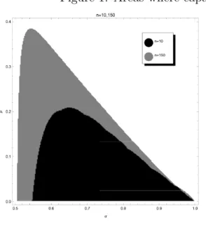
condition is much harder to obtain, so we investigate this question numerically. Figure 1(a),
where all consumers are uninformed, shows that the region where restricting capacity can be
optimal is larger when there are many consumers. There is also an interesting interaction
between signal precision and the prior. When the signal is very imprecise (α ≈ 1/2), it is
relatively likely that at least half of the consumers will buy, regardless of the state, so the seller
will remain unconstrained and bet on generating a positive cascade. As signal precision increases,
an unconstrained seller becomes increasingly likely to experience a negative cascade when the
state is bad, so the seller will restrict capacity for sufficiently small β. A further increase in
signal precision makes restricting capacity increasingly helpful in the bad state, but increasingly
harmful in the good state, as a correct positive cascade is then likely without a constraint. The
first effect dominates for intermediate α, but the second effect dominates when α is sufficiently
large, because an incorrect positive cascade is only likely given a very low constraint, which
would dramatically reduce profits in the good state. Figure 1(b) depicts the optimal level of
capacity for these different parameter values.
Figures 1(c) and 1(d) show how the presence of informed consumers affects the seller’s
incentive to restrict capacity. It does so indirectly, via the way that m≥1 or >0 changes the
probabilities Qi
ω. It also does so directly, via the way that m ≥ 1 or >0 explicitly enter the
profit functions, because informed consumers can potentially reverse incorrect cascades. This
latter direct effect generates one of our two channels by which a capacity constraint can increase
profits: by masking the choice of informed consumers not to buy, which can prevent an incorrect
positive cascade from being reversed.
The medium-gray bell-shaped area in figures 1(c) and 1(d) shows when restricting capacity
shifts the bell shape to the left (lighter-grey area). More purchase decisions in early cohorts
are then likely to reflect the true state; this has an ambiguous effect on the incentive to restrict
capacity, as it is analogous to an increase in signal precision. In contrast, the direct effect
of having informed consumers unambiguously makes restricting capacity more attractive. The
relevant region now consists of both the lighter-grey area and the dark area above, reflecting
how informed consumers can quickly reverse profitable positive cascades, but only if the seller
is unconstrained.11
4
Further Results
4.1
General Profit Functions and Learning in the Long Run
The profit functions (9) and (11) for a constrained seller apply to situations where a single
sell-out triggers a positive cascade. For given prior beliefs, signal accuracy, and capacity, we can
always find a value of the consumers’ outside option such that one sell-out is indeed sufficient.
But more generally, multiple sell-outs may be necessary to trigger a cascade, in particular when
capacity is relatively low. Might the seller have an incentive to set such a capacity, which delays
the start of a positive cascade, but also increases the probability of selling out?
To address this issue, we write down general profits function for a seller with capacity K, in
both the deterministic and stochastic setting. Recall from (5) that γ(l, K) denotes the belief of
a consumer in cohort l+ 1 that the state is good, after sell-outs in all l previous periods, and
after receiving a bad signal. Let L = {l : γ(l, K) > r}, which is non-empty by Lemma 3, and
denote the smallest element ofL byL: the number of consecutive sell-outs required as of period
1, given capacity K, in order to generate a positive cascade. The value of Lis decreasing in K,
since selling out at higher capacity presents stronger evidence that the state is good.
11In the light-grey area, the impact of informed consumers on probabilities is sufficient to justify some capacity
constraint. That is,πQui < πQ
i
c (K) holds for some K. In the dark area, this inequality does not hold, but the
seller still prefers to be constrained due to the fact that non-rationed informed consumers might stop incorrect cascades, so thatπi
Figure 1: Areas where capacity restriction can be optimal.
(a) m = 0 or ε= 0, area where constraint is optimal for somer, δ.
(b) OptimalK,m= 0 orε= 0.
Let ηωi = P2n
j=KQ i
ω(j), i ∈ {det, sto}, denote the probability of a sell-out, given state ω ∈
{G, B}. Let Si
B =
PK−1
j=0 jQ
i
B(j) denote expected sales in a given period conditional on not
selling out, when the state is bad; similarly, let
˜
SGdet≡
K−1
X
j=0
QdetG (j)
j+δm+ δ 2K 1−δ
,
denote expected sales as of a period where a sell-out does not occur, and when the state is good.
Expected profits given capacity K and L≥1, in the deterministic setting, are
πcdet(K) = β
1−(δηdet G )L
1−δηdet G
( ˜SGdet+ηdetG K) + (δηdetG )L K 1−δ
+
(1−β)
1−(δηBdet)L 1−δηdet
B
(SBdet+ηBdetK) + (δηBdet)L K 1−δ
. (12)
When the state is bad, the seller experiences L consecutive sell-outs each with probabilityηdetB ,
which triggers a positive cascade and yields revenue of K in all periods. Otherwise, the seller
earns SBdet in the first period where it fails to sell out, and then zero in all later periods. The
situation is similar when the state is good, except the probability of a sell-out in each period is
ηdetG rather thanηBdet, and a seller that fails to sell out will earn ˜SGdet on average as of that period.
As expected, expression (12) reduce to (9) if L = 1, so if one sell-out is sufficient to trigger a
cascade.
Similarly, denote
˜
SGsto≡
K−1
X
j=0
QstoG (j) j+δ
P2n
i=1 2n
i
εi(1−ε)2n−i(min{i, K}+1Kδ−δ) 1−(1−ε)2nδ
!
,
and
RstoB = K 1−δ −
P2n
i=2n−K+1 2n
i
εi(1−ε)2n−i(i−2n+K+ Kδ
1−δ)
1−P2n−K
i=0 2n
i
εi(1−ε)2n−iδ .
Expected profits given capacity K and L≥1, in the stochastic setting, are
πcsto(K) =β
1−(δηGsto)L 1−δηsto
G
( ˜SGsto+ηGstoK) + (δηGsto)L K 1−δ
+
(1−β)
1−(δηstoB )L 1−δηsto
B
(SBsto+ηstoB K) + (δηBsto)LRstoB
Figure 2: Seller profits and L.
0 2 4 6 8 10 K
2.0 2.2 2.4 2.6 2.8 3.0 3.2 π
n=10, m=0,δ=0.8,α=0.9,β=0.001, r=0.008
πU πC(K)
(a)
34
9
4 3
2 1 1 1 1 1
0 2 4 6 8 10 K
0 5 10 15 20 25 30 35
π
n=10, m=0,δ=0.8,α=0.9,β=0.001, r=0.008
L
(b)
which reduces to (11) ifL= 1.
Holding capacity constant at K, profits in both settings are strictly decreasing in L, because
a large L means that more sell-outs are required to trigger a positive cascade. However, L
depends on K, and the seller may in fact want to set a sufficiently low capacity that results in
L > 1. Such a low capacity makes a sell-out in each period more likely, and thus reduces the
probability in each period that a negative cascade begins. Indeed, Figure 2 shows parameter
values for which the seller prefers to setK = 1, so that L= 34 sell-outs are necessary to trigger
a cascade.
Figure 2 also shows that profits might not be quasi-concave in K and sudden jumps can
occur. An increase in K gives a lower chance of a sell-out in any given period, higher sales
conditional on selling out or on being in a positive cascade, and may also mean that fewer
sell-outs are necessary for the cascade to begin. The balance between these three forces may
sometimes swing sharply. In the figure, an increase in K from 5 to 6 reduces the number of
sell-outs necessary to start a cascade from L= 2 to L= 1, which pushes up profits.
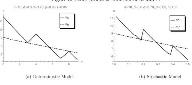
Figure 3 illustrates how profits depend on how many consumers are informed. Profit
func-tions (12) and (13) are directly decreasing inmandεrespectively, givenβ <1/2, since informed
consumers are more likely to know that the state is bad rather than good. Nonetheless,
Figure 3: Seller profits as function of m and ε.
0 2 4 6 8 m
7 8 9 10 11 π
n=10,δ=0.8α=0.78,β=0.05, r=0.05
πU πC
(a) Deterministic Model
0.0 0.1 0.2 0.3 0.4 0.5 ϵ 6
7 8 9 10 11
π
n=10,δ=0.8α=0.78,β=0.05, r=0.05
πU πC
(b) Stochastic Model
of sell-outs at a given capacity that are required to trigger a positive cascade. For example,
an increase in m can lead the seller to choose lower K, because one sell-out will now trigger a
cascade at this lower capacity, and result in higher profits.
Whereas our main focus has been on how restricting capacity affects the present value of seller
profits, we now briefly consider consumer learning and profits in the long run. In the stochastic
model with > 0, uninformed consumers will eventually learn the true state, regardless of
whether the seller is constrained. Even if an initial sell-out at low capacity immediately triggers
a positive cascade, in each later period enough informed consumers may arrive to yield excess
capacity if the state is bad. Thus, the probability that an incorrect cascade continues up until
periodT will become vanishingly small, asT becomes large. The ex ante probability of a correct
positive cascade in the long run is simply β, the prior probability that the state is good, and
the probability of a correct negative cascade is 1−β.
The same conclusion applies in the deterministic model with m ≥ 1 if the seller is
uncon-strained, where the choices of informed consumers will reveal the state immediately following
the start of any cascade. If the seller restricts capacity toK ≤n, the state is also revealed after
the start of a negative cascade, but not after a positive one. As described earlier in the analysis,
an incorrect positive cascade will yield sell-outs in every period, so that no further information
The probability of an incorrect positive cascade, given capacityKand critical number of
sell-outs L, is (1−β)(ηdet
B )L (we omit the argument K for simplicity), where ηBdet =
P2n
j=KQ det B (j)
is the probability of a sell-out when the state is bad. Notice that (1−β)(ηdetB )L is also the
probability that consumers will fail to learn in the long run when some consumers are informed.
This probability depends on the seller’s choice of K and also on various model parameters:
directly on β, directly on α, K, and m through ηdet
B , and indirectly on α, β, r, and K through
L.
To derive an upper bound on this probability, define Γ(l, K) as the public belief that the
state is good, conditional on sell-outs at capacity K in the first l periods. That is
Γ(l, K) = 1
1 + 1−ββh
P2n
j=KQdetB (j) P2n
j=KQdetG (j)
il,
where r < γ(L, K)<Γ(L, K) follows from (5) and the definition ofL.
For m≥1, we can write
β(ηGdet)L+ (1−β)(ηBdet)LΓ(L, K) +β(1−(ηdetG )L)×1 + (1−β)(1−(ηdetB )L)×0 = β.
That is, the average public belief conditional on i) a positive cascade triggered by Lsell-outs in
either state, which results in Γ(L, K); ii) an eventual positive cascade following an initial failure
to sell out, where informed consumers’ actions reveal that the state is good; and iii) a negative
cascade following an initial failure to sell out, where informed consumers’ actions reveal that
the state is bad; weighted by the probability of these different cascades occurring, must equal
the prior β. Combining with r <Γ(L, K)<1 yields
β(ηGdet)L+ (1−β)(ηBdet)L+β(1−(ηGdet)L)< β r,
so the probability of a positive cascade is bounded above by β/r.12 This bound is informative
whenr > β, and becomes increasingly so if consumers’ outside option is good or the prior is low.
12The same bound applies form= 0, which in that case follows from [β(ηdet
G )L+ (1−β)(ηBdet)L]Γ(L, K)< β
Thus, the bound will tend to be more informative when the state is likely bad, which is when
our earlier results suggested the seller may be particularly interested in restricting capacity.
It follows that the probability of an incorrect positive cascade is at mostβ/r−β =β(1/r−1).
Similarly, the likelihood ratio of an incorrect positive cascade, relative to a correct positive
cascade, is at most 1/r−1. The better the outside option, the less likely that a positive cascade
will be incorrect. Intuitively, when consumers’ outside option is very good, a positive cascade
can only occur after many sell-outs (or fewer sell-outs but at a high capacity), which is unlikely
to occur in the bad state.
The long-run per period expected profits of a constrained seller is bounded by the probability
of a positive cascade times its capacity,πdet,LR
c (K)<(β/r)K. The long-run per period expected
profits of an unconstrained seller is justπdet,LRu = 2nβ. This allows us to formulate the following
result regarding the optimal choice of capacity.
Proposition 2. Consider the deterministic model. For δ sufficiently close to 1, only capacity
constraints K > 2nr can be profitable relative to being unconstrained: πdet
u > πdetc (K) for all
K ≤2nr.
An immediate implication of Proposition 2 is that a sufficiently patient seller, facing
con-sumers with outside option r > 1/2, will never use a capacity constraint as a way to increase
the probability of triggering a positive cascade. Rather than restricting capacity toK ≤n, such
a seller would prefer to remain unconstrained.13
4.2
Pricing
We now briefly discuss how pricing can affect our results. The seller’s optimization problem,
seen only as a function of capacity, is complicated by the fact that profits are not necessarily
quasi-concave inK. Considering both capacity and price complicates matters further still, since
the seller’s optimal price is directly linked to its capacity choice. To illustrate the main features
13There is also the possibility of restricting capacity toK= 2n−m > n simply to hide informed consumers’
of the optimal pricing problem, and maintain tractability, we proceed as follows. First, we
assume the seller sets a price at t =−1 that is fixed for all periods. Second, we normalize the
consumer’s outside opt ion to zero and now interpret r as the price, so the consumer problem is
exactly as before, and the seller’s problem involves the optimal choice of r. Third, we focus on
the baseline case with m = 0 (ε = 0), which makes our framework more similar to Bose et al.
(2008), and we compute the optimal price for a constrained seller numerically.14
In line with Bose et al. (2008), an unconstrained seller can choose a pooling price such that
both consumers with good and bad signals want to buy:
rp =
β(1−α)
β(1−α) +α(1−β),
which yields profits
Πp =
2n
1−δrp.
Any lower pooling price r < rp would not increase demand and would result in lower profits.15
Alternatively, an unconstrained seller can charge a separating price such that only consumers
with good signals want to buy:
rs=
αβ
αβ+ (1−α)(1−β).
Doing so yields profits
Πs =πudetrs,
withπdet
u given by (8) withm = 0. Any higher pricer > rs would lead to zero sales, whereas any
lower separating price rp < r ≤rs would not increase demand. The optimal pricing problem is
solved by a direct comparison of Πp and Πs.
For a constrained seller, we only consider separating prices, rp < r ≤ rs, since a seller that
charged a pooling price would prefer to be unconstrained. Given capacity K and separating
14That being said, the fact that Bose et al. (2008) consider dynamic rather than static pricing, and do not
consider restricted capacity, limits the comparability of our results.
15Ifm≥1, then in the good state all consumers would still buy at pricer
pin all periods, but in the bad state
price r, profits are
Π =πdetc (K)r, (14)
with πdet
c (K) given by (12) with m= 0. The higher the separating pricer, the more sell-outsL
are required to trigger a positive cascade, so πdet
c (K) depends on r.
To say more about the optimal price given capacityK, defineLmaxas the largest value ofLfor
whichγ(L−1, K)< rs. That is, consumers with good signals in the first cohort will want to buy
at pricer =γ(L, K) if and only ifL≤Lmax−1.16 Demand is independent of price wheneverr∈
(γ(L, K), γ(L+ 1, K)), so the optimal price is an element of{γ(1, K), . . . , γ(Lmax−1, K), rs}.17
The seller faces the following trade-off: charge a higher price and wait for more sell-outs to
trigger a cascade, or charge a lower price and hope to trigger a cascade more quickly. Figure 4
illustrates how this trade-off is usually resolved in favour of a higher price and longer waiting
for a positive cascade, unless K is very close ton and bothα and δ are low.
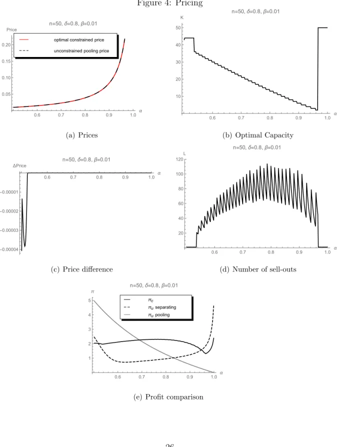
Panels 4(a) and 4(c) show that the optimal price is often equal to the unconstrained
sepa-rating price rs, regardless of which capacity K ≤ n the seller finds to be optimal. Differences
between these prices, when they do exist, are very small in magnitude. Thus, the seller’s problem
will often boil down to whether restricting capacity increases expected demand, holding price
fixed at r=rs. This suggests that the conclusions from our main analysis, where the seller only
optimized over capacity, will tend to carry through to a model with pricing.
Given the relatively high optimal price, multiple sell-outs L ≈ Lmax are often required to
start a cascade, where panel 4(d) also shows a saw-like pattern. As signal precision increases,
the seller requires fewer sell-outs to trigger a cascade for a given capacity, which pushesLdown.
But as precision increases, panel 4(b) shows that the seller will sometimes reduce its capacity,
so that more sell-outs are required to trigger a cascade, which pushes L sharply up. Panel 4(e)
suggests that the overall comparison of profits is qualitatively similar to what we had before: the
seller finds it optimal to restrict capacity when the signal accuracyα is neither too high nor too
low, similar to Figure 1. The only difference is that for low signal accuracy, an unconstrained
16Such a valueL
max exists by Lemma 5. 17Notice thatL
Figure 4: Pricing
0.6 0.7 0.8 0.9 1.0 α 0.05
0.10 0.15 0.20 Price
n=50,δ=0.8,β=0.01
unconstrained pooling price optimal constrained price
(a) Prices
0.6 0.7 0.8 0.9 1.0 α
10 20 30 40 50 K
n=50,δ=0.8,β=0.01
(b) Optimal Capacity
0.6 0.7 0.8 0.9 1.0 α
-0.00004 -0.00003 -0.00002 -0.00001
ΔPrice
n=50,δ=0.8,β=0.01
(c) Price difference
0.6 0.7 0.8 0.9 1.0 α
20 40 60 80 100 120 L
n=50,δ=0.8,β=0.01
(d) Number of sell-outs
0.6 0.7 0.8 0.9 1.0 α
1 2 3 4 5 π
n=50,δ=0.8,β=0.01
πupooling πuseparating πc
seller now prefers the pooling price.
5
Conclusions
In this paper, we show that a firm may benefit from restricting capacity, to trigger herding
behav-ior from consumers and increase future sales. Limiting capacity results in coarser information,
as consumers who observe a sell-out attach positive probability to all levels of demand that
exceed capacity. The results show that two main mechanisms the literature suggests may help
avoid pathological social learning outcomes, ‘guinea pigs’ and unbounded private signals, can
fail to do so, if the firm is able to manipulate the learning environment by a simple instrument
such as limiting capacity.
Our results rely on the idea that consumers can observe sales and capacity. This is reasonable
in many markets, e.g. restaurants, sports and concert tickets, and limited car editions, where
sales and capacity are often widely known, but the extent of any excess demand is not. Product
scarcity should also affect learning in other settings, but in a way that depends precisely on
what consumers can observe. For example, it will matter if concert promoters can ‘paper the
house’ by quietly filling seats for free, or if sales figures for certain consumer products become
widely reported precisely because shortages occurred. Our mechanism will also continue to apply
in situations where capacity is exogenous, although our main results will then have a slightly
different interpretation; namely, that a firm that must limit production, or use a small venue,
may do just as well (or better) than a firm that is not similarly constrained.
Restricting capacity would still help to trigger positive cascades if consumers were partially
sophisticated, and believed that others always followed their own private signals (see, e.g., Eyster
and Rabin (2010), Gagnon-Bartsch and Rabin (2017), and Dasaratha et al. (2018)). Just as
in our analysis, an initial sell-out would result in a cascade if it revealed high enough demand
from consumers in the first cohort. If capacity was low, then some consumers in the second
cohort might be close to indifferent about buying, as the sell-out would then provide only weak
become increasingly confident that the state is good after observing more and more sell-outs,
and become increasingly willing to buy.
In line with most work on social learning, our seller is not privately informed, but an alterative
would be to assume that the seller receives its own private binary signal about quality. The full
analysis of such a model is beyond the scope of this paper. However, it is clear that if the seller’s
signal precision is low, then there can exist an equilibrium where the seller restricts capacity.
Our model can be viewed as a limit case of such a pooling equilibrium where the seller’s signal
is completely uninformative. A separating equilibrium would require that period-1 consumers
always follow their own signal, along with a standard incentive compatibility condition where
the seller only wants to restrict capacity after a bad signal. Notice the connection here with a
key result in our analysis: that it is precisely a seller that expects relatively low sales that can
References
Daron Acemoglu, Munther A Dahleh, Ilan Lobel, and Asuman Ozdaglar. Bayesian learning in
social networks. The Review of Economic Studies, 78(4):1201–1236, 2011.
Masaki Aoyagi. Optimal sales schemes against interdependent buyers. American Economic
Journal: Microeconomics, 2(1):150–82, 2010.
Pak Hung Au. Dynamic information disclosure. The RAND Journal of Economics, 46(4):
791–823, 2015.
Robert J Aumann, Michael Maschler, and Richard E Stearns. Repeated games with incomplete
information. MIT press, 1995.
Abhijit Banerjee and Drew Fudenberg. Word-of-mouth learning.Games and Economic Behavior,
46(1):1–22, 2004.
Abhijit V Banerjee. A simple model of herd behavior. The Quarterly Journal of Economics,
pages 797–817, 1992.
James Best and Daniel Quigley. Persuasion for the long run. 2017.
Manaswini Bhalla. Waterfall versus sprinkler product launch strategy: Influencing the herd.
The Journal of Industrial Economics, 61(1):138–165, November 2013.
Sushil Bikhchandani, David Hirshleifer, and Ivo Welch. A theory of fads, fashion, custom, and
cultural change as informational cascades. Journal of Political Economy, pages 992–1026,
1992.
Jacopo Bizzotto, Jesper R¨udiger, and Adrien Vigier. Dynamic persuasion with outside
infor-mation. 2018.
Subir Bose, Gerhard Orosel, Marco Ottaviani, and Lise Vesterlund. Dynamic monopoly pricing
Subir Bose, Gerhard Orosel, Marco Ottaviani, and Lise Vesterlund. Monopoly pricing in the
binary herding model. Economic Theory, 37(2):203–241, 2008.
Steven Callander and Johannes H¨orner. The wisdom of the minority. Journal of Economic
theory, 144(4):1421–1439, 2009.
Bo˘ga¸chan C¸ elen and Shachar Kariv. Observational learning under imperfect information.Games
and Economic Behavior, 47(1):72–86, 2004.
Yeon-Koo Che and Johannes Horner. Optimal design for social learning. 2015.
Krishna Dasaratha, Benjamin Golub, and Nir Hak. Social learning in a dynamic environment.
2018.
Laurens G Debo, Christine Parlour, and Uday Rajan. Signaling quality via queues.Management
Science, 58(5):876–891, 2012.
Patrick DeGraba. Buying frenzies and seller-induced excess demand. The RAND Journal of
Economics, pages 331–342, 1995.
Piotr Dworczaky and Giorgio Martiniz. Optimal dynamic information provision. 2018.
Jeffrey C Ely. Beeps. American Economic Review, 107(1):31–53, 2017.
Erik Eyster and Matthew Rabin. Naive herding in rich-information settings.American economic
journal: microeconomics, 2(4):221–43, 2010.
Tristan Gagnon-Bartsch and Matthew Rabin. Naive social learning, mislearning, and unlearning.
2017.
Matthew Gentzkow and Emir Kamenica. Costly persuasion. American Economic Review, 104
(5):457–62, 2014.
Matthew Gentzkow and Emir Kamenica. Competition in persuasion. The Review of Economic
Matthew Gentzkow and Emir Kamenica. Bayesian persuasion with multiple senders and rich
signal spaces. Games and Economic Behavior, 104:411–429, 2017.
David Gill and Daniel Sgroi. Sequential decisions with tests. Games and economic Behavior,
63(2):663–678, 2008.
David Gill and Daniel Sgroi. The optimal choice of pre-launch reviewer. Journal of Economic
Theory, 147(3):1247–1260, 2012.
Benjamin Golub and Evan D Sadler. Learning in social networks. 2017.
Antonio Guarino, Heike Harmgart, and Steffen Huck. Aggregate information cascades. Games
and Economic Behavior, 73(1):167–185, 2011.
Helios Herrera and Johannes H¨orner. Biased social learning. Games and Economic Behavior,
80:131–146, 2013.
Emir Kamenica and Matthew Gentzkow. Bayesian persuasion. American Economic Review,
101(6):2590–2615, 2011.
Anton Kolotilin and Andriy Zapechelnyuk. Persuasion meets delegation. 2018.
Anton Kolotilin, Tymofiy Mylovanov, Andriy Zapechelnyuk, and Ming Li. Persuasion of a
privately informed receiver. Econometrica, 85(6):1949–1964, 2017.
Ilan Kremer, Yishay Mansour, and Motty Perry. Implementing the wisdom of the crowd.Journal
of Political Economy, 122(5):988–1012, 2014.
Ting Liu and Pasquale Schiraldi. New product launch: herd seeking or herd preventing?
Eco-nomic Theory, 51(3):627–648, 2012.
Ilan Lobel and Evan Sadler. Information diffusion in networks through social learning.
Theo-retical Economics, 10(3):807–851, 2015.
Marc M¨oller and Makoto Watanabe. Advance purchase discounts versus clearance sales. The
Economic Journal, 120(547):1125–1148, 2010.
Ignacio Monz´on. Aggregate uncertainty can lead to incorrect herds. American Economic
Jour-nal: Microeconomics, 9(2):295–314, 2017.
Ignacio Monz´on and Michael Rapp. Observational learning with position uncertainty. Journal
of Economic Theory, 154:375–402, 2014.
Volker Nocke and Martin Peitz. A theory of clearance sales. The Economic Journal, 117(522):
964–990, 2007.
Dmitry Orlov, Andrzej Skrzypacz, and Pavel Zryumov. Persuading the principal to wait. 2018.
HG Parsa, John T Self, David Njite, and Tiffany King. Why restaurants fail. Cornell Hotel and
Restaurant Administration Quarterly, 46(3):304–322, 2005.
J´erˆome Renault, Eilon Solan, and Nicolas Vieille. Optimal dynamic information provision.
Games and Economic Behavior, 104:329–349, 2017.
Amin Sayedi. Pricing in a duopoly with observational learning. 2018.
Daniel Sgroi. Optimizing information in the herd: Guinea pigs, profits, and welfare. Games and
Economic Behavior, 39(1):137–166, 2002.
Lones Smith and Peter Sørensen. Pathological outcomes of observational learning.Econometrica,
68(2):371–398, 2000.
Lones Smith and Peter Norman Sorensen. Rational social learning by random sampling. 2013.
Axel Stock and Subramanian Balachander. The making of a hot product: A signaling
explana-tion of marketers scarcity strategy. Management Science, 51(8):1181–1192, 2005.
Ivo Welch. Sequential sales, learning, and cascades. The Journal of finance, 47(2):695–732,
1992.
Appendix: Proofs
Proof of Lemma 1. Deterministic model. Consider Qdet
G (j) given by (1) and QdetB (j) given by
(2). Clearly, QdetB (j) Qdet
G (j)
= 0 if 2n−j ≤m−1, and for 2n−j ≥m
Qdet B (j)
Qdet G (j)
=
(j−m)! (2n−m−j)!
(2n−j)!
j!
α2(n−j)(1−α)2(j−n)
which is decreasing in j and equals to 1 when j =n. Moreover, for j =n−1 we get
Qdet
B (n−1)
Qdet
G (n−1)
= n(n+ 1) (n−m−1)(n−m)
α2 (1−α)2 >
α2 (1−α)2
and for j =n+ 1 we get
Qdet
B (n+ 1)
Qdet
G (n+ 1)
= (n−m−1)(n−m)
n(n+ 1)
(1−α)2
α2 <
(1−α)2
α2
Now,
QdetG (2n−j) =
2n−m
2n−j−m
α2n−j−m(1−α)j =
2n−m
2n−j−m
α2n−j−m(1−α)j =QdetB (j).
Finally,
QdetG (j)
Qdet
G (2n−j)
= Q
det G (j)
Qdet B (j)
>1
for all j > n+ 1 as the ratio on the right-hand side is increasing forj > m and QdetG (n) Qdet
B (n)
= 1.
Stochastic model.
Consider Qsto
G (j) given by (3) and QstoB (j) given by (4).
Letξ ≡α+ε−αε, and note that ξ∈(1/2,1). Therefore, expressions forQsto
ω (j) are exactly
as in the deterministic model with m= 0 and α replaced with ξ. Moreover, sinceξ > α we get
ξ
1−ξ > α
Proof of Lemma 2. Consider t = 2. Note, that
P(G|n+ 1, b) = 1
1 + 1−ββ1−ααQiB(n+1) Qi
G(n+1)
≥ 1
1 + 1−ββ1−α α
=P(G|g)> r
where the first inequality follows from QiB(n+1) Qi
G(n+1)
≤ 1−α α
2
, i ∈ {det, sto}. Thus, the belief of a
consumer that quality is good after observing S1 ≥ n+ 1 and s =b is better than P(G|g), so
the consumer should buy regardless of her private information. In a similar way we get
P(G|n−1, g) = 1
1 + 1−ββ1−ααQiB(n−1) Qi
G(n−1)
≤ 1
1 + 1−ββ1−αα =P(G|b)< r
due to QiB(n−1) Qi
G(n−1)
≥ α
1−α
2
. Finally,P(G|n, b) =P(G|b) andP(G|n, g) = P(G|g) due to QiB(n) Qi
G(n)
= 1,
so if S2 =n consumer should follow her own signal. Now, consider t >2. Suppose that for all
t0 < t−1, St0 = n holds. Due to Q i B(n) Qi
G(n)
= 1, this implies that in all cohorts consumers have
followed their own signal. Thus, ifSt−1 =n consumers in cohorttalso must follow their signals.
Suppose that St−1 > n. In this case
P(G|S1, . . . , St−1;b) =
β(1−α)Qi
G(St−1)[QiG(n)]t −2
β(1−α)Qi
G(St−1)[QGi (n)]t−2+ (1−β)αQiB(St−1)[QiB(n)]t−2
=
1
1 + 1−ββ1−ααQiB(St−1) Qi
G(St−1)
> r
so consumers should buy. Similarly, if St−1 < n we get P(G|S1, . . . , St−1;g)< r and consumers
should not buy.
Now, suppose there exists first t0 < t−1 such thatSt0 6=n. If St0 < n consumers in the next
cohort should not buy and the cascade starts. If for allτ ∈[t0+ 1, t−1]Sτ = 0, then consumers
do not gain any additional information and should abstain. If for some τ ∈[t0+ 1, t−1]Sτ >0
the purchase must come from an informed consumer and consumers in later cohorts should buy.
In a similar vein if St0 > n then the positive cascade starts, it persists if for all τ ∈[t0+ 1, t−1]
Sτ = 2n. It is otherwise reversed, as the decision not to buy comes from an informed consumer,
Proof of Lemma 3. From (5) it is sufficient to show that P2n
j=KQ i
B(j) <
P2n
j=KQ i
G(j), i ∈
{det, sto}. Note, that since for all j > n + 1 we have Qi
G(j) > QiG(2n − j) we obtain
PK−1
j=0 Q
i
G(j) <
P2n
j=2n−K+1Q
i
G(j). By adding
P2n−K
j=K Q i
G(j) we obtain that
P2n−K
j=0 Q
i G(j) <
P2n
j=KQ i
G(j). By changing the summation order on the left-hand-side we obtain
P2n
j=KQ i G(2n−
j)<P2n
j=KQ i
G(j). Finally, due to QiB(j) =QiG(2n−j) we obtain
P2n
j=KQ i B(j)<
P2n
j=KQ i G(j).
Proof of Lemma 4. As shown in the proof of Lemma 3, P2n
j=KQ i
B(j) <
P2n
j=KQ i
G(j), i ∈
{det, sto}. Thus,
γ(1, K) = 1 1 + 1−ββ1−αα
P2n j=KQiB(j) P2n
j=KQiG(j)
> 1
1 + 1−ββ1−αα =P(G|b)
AsP(G|b)> r, the conditionγ(1, K)> rcan always be satisfied by choosingr sufficiently close
toP(G|b).
Proof of Lemma 5. For simpler notation we are going to omit thes superscript in our
prelimi-nary steps and work with generic Q. Rewrite (6) as
[1−δQ(n)]πuQ =S1+
δ
1−δ2nS2, (15)
where S1 =
P2n
j=1jQ(j) and S2 =
P2n
j=n+1Q(j). Note that as long as Q(n) < 1, the term [1−δQ(n)] is bounded away from 0 for δ <1. In a similar way,
πcQ(K) =S1− 2n
X
j=K
(j−K)Q(j) + δ 1−δK[
n−1
X
j=K
Q(j) +Q(n) +S2]>
S1 −(2n−K)[
n−1
X
j=K
Q(j) +Q(n) +S2] +
δ
1−δK[
n−1
X
j=K
Q(j) +Q(n) +S2],
where the inequality follows from replacing all terms (j −K) with the larger term 2n −K.
Moreover, for δ > 2n2−nK the penultimate term is smaller than the last one, and thus
πcQ(K)> S1 +
δK −(2n−K)(1−δ)