Online Repositioning in Bike Sharing Systems
Meghna Lowalekar, Pradeep Varakantham, Supriyo Ghosh, Sanjay Dominik Jena
†, Patrick Jaillet
‡ School of Information Systems, Singapore Management University†
Département de management et technologie, École des sciences de la gestion (ESG) UQAM ‡
Dept. of Electrical Engineering and Computer Science, Massachusetts Institute of Technology, USA
[email protected], [email protected], [email protected],[email protected],[email protected]
Abstract
Due to increased traffic congestion and carbon emissions, Bike Sharing Systems (BSSs) are adopted in various cities for short distance travels, specifically for last mile transportation. The success of a bike sharing system depends on its ability to have bikes available at the "right" base stations at the "right" times. Typically, carrier vehicles are used to perform repo-sitioning of bikes between stations so as to satisfy customer requests. Owing to the uncertainty in customer demand and day-long repositioning, the problem of having bikes avail-able at the right base stations at the right times is a chal-lenging one. In this paper, we propose a multi-stage stochas-tic formulation, to consider expected future demand over a set of scenarios to find an efficient repositioning strategy for bike sharing systems. Furthermore, we provide a Lagrangian decomposition approach (that decouples the global problem into routing and repositioning slaves and employs a novel DP approach to efficiently solve routing slave) and a greedy on-line anticipatory heuristic to solve large scale problems effec-tively and efficiently. Finally, in our experimental results, we demonstrate significant reduction in lost demand provided by our techniques on real world datasets from two bike sharing companies in comparison to existing benchmark approaches.
1
Introduction
Bike Sharing systems (BSSs) are rapidly becoming a dom-inant mode of transportation for short distance trips in var-ious cities. The use of bicycle as a mode of transportation helps in decreasing traffic congestion and carbon emissions that has been increasing due to excess private vehicle usage. Some of the popular bike sharing systems include Capital Bikeshare in Washington DC, Hubway in Boston, Bixi in Montreal, and Vélib in Paris. A bike sharing system typi-cally has a set of base stations that are strategitypi-cally placed throughout a city and each station has a fixed number of docks. At the start of the day, each station is stocked with a predetermined number of bikes. Customers can pick and drop bikes from any station and are charged depending on the hiring duration.
As the customers move according to their own needs, dur-ing the course of the day there will be starvation at some sta-tions and congestion at some stasta-tions. To rebalance the avail-ability of bikes, companies employ carrier vehicles to move bikes between stations. There has been extensive research on static repositioning approaches (Schuijbroek, Hampshire,
Copyright c2017, Association for the Advancement of Artificial Intelligence (www.aaai.org). All rights reserved.
and van Hoeve 2017; Chemla, Meunier, and Calvo 2013; Raviv, Tzur, and Forma 2013). These approaches perform repositioning only at the beginning of the day, when the movements of bikes by the customers are negligible, to en-sure desired distribution of bikes across different stations. But they do not consider stations getting imbalanced during the day. Hence there is a need to focus on dynamic reposi-tioning of bikes (Contardo, Morency, and Rousseau 2012; Ghosh et al. 2015; 2017) during the day.
Shu et al. (2013) provide an optimization model for dy-namic repositioning of bikes, but they do not consider rout-ing of carrier vehicles. Ghosh et al. (2015; 2017) consider the problem of dynamic repositioning of bikes along with the problem of finding the routing policy for carrier vehicles. They provide an offline policy generation approach based on mean demand computed from the historical data. To over-come the inherent complexity of the problem, they propose a decomposition and abstraction based approach. While the offline policy provides significant improvement over static repositioning approaches, it is unable to consider the chang-ing demand scenarios in real time. Recently Ghosh and Varakantham (2017) propose a novel dynamic reposition-ing approach by combinreposition-ing optimization and mechanism de-sign, to reduce carbon footprint using bike trailers. Ghosh, Trick, and Varakantham (2016) provide an online approach to compute dynamic repositioning and routing policy. The focus of their work is on providing a robust approach which optimizes for the worst case scenario. While robust policies provide guarantees for the adversarial inputs, they do not work well when demand follows an expected distribution and hence, we do not provide an experimental comparison.
a greedy online anticipatory heuristic approach to improve scalability. Finally, we provide an exhaustive comparison of our approaches against multiple benchmarks on two real world datasets.
2
Model
In this section, we provide a generic model for represent-ing the problem of repositionrepresent-ing and routrepresent-ing while consid-ering demand uncertainty in bike sharing systems. We ex-tend the expected demand based model of Dynamic Reposi-tioning and Routing Problem (DRRP) provided by Ghosh et al. (2015). Here, we provide the Dynamic Reposition-ing and RoutReposition-ing Problem with Demand Uncertainty (DR-RPDU), that considers multiple samples of demand at dif-ferent stations and timesteps.
DRRPDU is formally defined using the following tuple:
D
S,V, F, C#, C∗, d, ξ, σ,X,∆, QE
• Sdenotes the set of stations.
• Vdenotes the set of carrier vehicles used for repositioning of bikes.
• F denotes samples of customer requests for the future timesteps withFt,kdenoting the set of customer requests in demand samplekat decision epocht. We useFs,st,t00,kto
denote the number of customer requests between stations
sands0 in samplekwhich start at decision epochtand end at decision epocht0.Ft,k
s denotes the total number
of customer requests originating at stationsand decision epochtin samplek.
• C# denotes the capacity of stations with Cs# denoting
capacity of stations.
• C∗ denotes the capacity of carrier vehicles withC∗
v
de-noting capacity of vehiclev.
• ddenotes the initial distribution of bikes at stations with
dsdenoting the initial number of bikes at stations. • ξdenotes the initial distribution of bikes in vehicle with
ξvdenoting the initial number of bikes in vehiclev. • σdenotes the distribution of carrier vehicles at stations.
σt
v(s)is set to 1, if vehiclevstarts from stationsat
deci-sion epochtand is 0 otherwise.
• Xt
sdenotes the additional number of bikes which will
be-come available at stationsat decision epocht1.
• ∆denotes the decision epoch duration in minutes.
• Qdenotes the lookahead period, i.e., the number of de-cision epochs for which request samples are considered.
Q∗∆gives the lookahead period duration in minutes. The goal in DRRPDU is to minimize the expected lost demand over multiple samples of demand scenarios over the entire time horizonQ∗∆. It should be noted that all elements of the DRRPDU tuple except Q and∆ can be populated directly from bike sharing datasets.Qand∆are typically decided by management based on observing movement of bikes.
1
This could be due to the bikes hired in previous decision epochs which are expected to return at decision epocht
Variable Description
y+,0
s,v Number of bikes picked up from stationsby
vehiclevat current decision epoch.
ys,v−,0 Number of bikes dropped at stationsby vehiclev
at current decision epoch.
ys,v+,t,k Number of bikes picked up from stationsby
vehiclevat decision epochtin sample k
ys,v−,t,k Number of bikes dropped at stationsby vehiclev
at decision epochtin sample k
ht,ks Bikes hired in samplekat stationsat epocht
gt,ks Bikes returned in samplekat stationsat epocht
Lt,ks Lost demand in samplekat stationsat epocht
dt,ks Number of bikes present at stationsat epocht
in samplek u0
v Number of bikes present in vehiclevat current
decision epoch.
ut,k
v Number of bikes present in vehiclevat epocht
in samplek zt,k
s,v Indicates whether vehiclevis present at stations
at decision epochtin sample k
m0s,v,t Indicates whether vehiclevmoves towardssat
current decision epoch and reachessatt mt,t0,k
s,v Indicates whether vehiclevmoves towardssatt
and reaches s at decision epocht0in samplek
Table 1: Notation
MSS ():
min 1
|F|
Q−1
X
t=0
X
k
X
s
Lt,ks (1)
s.t. Lt,ks ≥Fst,k−ht,ks :::∀s, t, k (2)
y+s,v,t,k+y
−,t,k
s,v ≤C
∗
v∗z t,k
s,v :::∀s, v, t >0, k (3)
zs,vt,k, m0s,v,t, mt,t
0
,k
s,v ∈ {0,1} (4)
Constraints (5)−(22)
Table 2:MSS Formulation
3
Multi-Stage Stochastic Optimization
We now formulate DRRPDU as a mixed integer linear opti-mization formulation. Unlike most current online reposition-ing approaches that are typically myopic (Pfrommer et al. 2014), this multi-stage stochastic (MSS) formulation con-siders future demand scenarios while optimizing reposition-ing of bikes. The variables used in MSS are described in Table 1. Table 2 presents the MSS formulation. Here are the key constraints that are not specific to only one of reposi-tioning and routing:Lost demand:Constraints (2) along with the objective
en-sure that lost demand at any station, at any decision epoch is the difference between demand and hired bikes.
Validity of Pickup/Dropoff:Constraints (3) ensure that a
ve-hiclevpicks or drops bikes from any stationsat any deci-sion epocht in any samplekif and only if the stationsis visited by vehicle at decision epochtin samplek.
Repositioning:
ht,ks ≤F t,k
s :::∀s, t, k (5)
h0s,k≤ds−
X
v
y+s,v,0+
X
v
ys,v−,0:::∀s, k (6)
ht,ks ≤d t,k
s −
X
v
y+s,v,t,k+
X
v
y−s,v,t,k:::∀s, t >0, k (7)
gt,ks ≤ t−1
X
t0=0
X
s0 hts00,k∗
Fst00,s,t,k
Fst00,k +Xt
s :::∀s, t >0, k (8)
dt,ks =d t−1,k
s −
X
v
ys,v+,t−1,k+
X
v
ys,v−,t−1,k−h t−1,k s
+gt,ks :::∀s, t >1, k (9)
d1s,k=ds−
X
v
y+s,v,0+
X
v
y−s,v,0−h 0,k
s +g
1,k
s :::∀s, k (10)
dt,ks ≤Cs#:::∀s, t, k (11)
X
v
y+s,v,0≤d 0 s;
X
v
ys,v−,0≤C #
s −d
0
s:::∀s (12)
X
v
ys,v+,t,k≤d t,k
s ;
X
v
ys,v−,t,k≤C #
s −d
t,k
s :::∀s, k, t >0 (13)
ut,kv =u t−1,k
v +
X
s
ys,v+,t,k−
X
s
ys,v−,t,k:::∀v, k, t >0(14)
u0v,k=ξv+
X
s
ys,v+,0−
X
s
y−s,v,0:::∀v, k (15)
ut,kv ≤C
∗
v:::∀v, k, t (16)
ys,v+,0+y
−,0
s,v ≤C
∗
v∗σ
0
v(s) :::∀s, v (17)
Table 3:Repositioning Constraints
or Routing. Table 3 presents the constraints related to the repositioning problem:
Hired bikes :Constraints (5)-(7) ensure that at any station at any decision epoch, the number of hired bikes is the mini-mum of available bikes at station and demand at station.
Returned bikes:Constraint (8) compute the number of
re-turned bikes at any station and decision epoch as the sum of bikes returned due to hiring at previous decision epochs (within formulation) and bikes which will be returned due to previous hires.
Bike availability:Constraints (9)-(11) ensure that the
num-ber of available bikes at any station at any decision epoch is less than the capacity of that station. At any station, at any decision epoch, the number of bikes available is calculated by considering hired bikes at previous decision epoch, bikes picked up/dropped by vehicles in previous decision epoch and bikes returned by customers in current decision epoch.
Station capacity:Constraints (12)-(13) ensure that the
ber of bikes picked up from any station is less than the num-ber of available bikes and the numnum-ber of bikes dropped at any station is less than the number of available free slots.
Vehicle capacity:The number of bikes present in any
ve-hicle v is calculated by considering bikes picked up and dropped by vehicle in current decision epoch and the number of bikes already present in the vehicle. Constraints (14)-(16) ensure that at any decision epoch, in any sample, the number
Routing:
zs,vt,k= t−1
X
t0=1
mts,v0,t,k+m 0,t
s,v+σ
t
v(s) :::∀s, v, t >0, k (18)
mt,ts,v0,k≤
X
s0
zst,k0,v∗δ
t,t0
s0,s,v:::∀s, v, t, k (19)
m0s,v,t ≤
X
s0 σ0v(s
0
)∗δ0s0,t,s,v:::∀s, v, t (20)
Q−1
X
t0=t+1
X
s
mt,ts,v0,k =
X
s0
zt,ks0,v:::∀v, t, k (21)
Q−1
X
t0=1
X
s
m0s,v,t0=
X
s0 σ0v(s
0
) :::∀v (22)
Table 4:Routing Constraints
of bikes in any vehiclevis less than capacity of vehicle. Table 4 contains the constraints related to routing prob-lem. These constraints ensure that there exists a valid path between vehicle positions at different decision epochs.m0,t s,v
variables are used to ensure that at current decision epoch, vehicle moves towards same station across all samples. All the constraints in this case ensure thatmovement of vehicles
are valid.
Constraint (18) ensure that a vehiclevis present at station s, at decision epoch t, in sample k, if and only if , either it is reaching stationsat decision epocht due to previous assignments (given byσt
v values) or if it is going to reach
stationsat decision epocht due to assignments which are part of current formulation. Constraints (19)-(20) ensure that a vehiclevstarts moving towards stations0at decision epoch
tand reachess0at decision epocht0, if at decision epochtit was present at some stations, such that the distance between
sands0can be covered in timet0−t. We use binary constants
δt,ts,s00,vto indicate if vehiclevstarting at stationsat decision
epoch t reaches station s0 exactly at decision epoch t0 or not. We assume a fixed travel time between stations based on average speed of vehicle so these binary constants can be calculated beforehand. Constraints (21)-(22) ensure that at any decision epoch, if a vehicle is present at some station, then it will start moving towards exactly one of the stations. A movement between the same station indicates vehicle is staying at the same station.
We solve the MSS optimization formulation online at each decision epoch to compute the repositioning and rout-ing strategy. At each decision epoch, distribution of bikes at stations and vehicle positions are updated based on actual re-alized customer requests and repositioning strategy executed by vehicles.
solve quickly. Decomposition across samples does not help in reducing computation time, as for problems with large number of stations, even for a single sample MSS takes a long time (thousands of seconds). Therefore, we extend the Lagrangian Dual Decomposition (LDD) (Fisher 1985) method proposed by Ghosh et al. (2015) for solving offline repositioning and routing problem in bike sharing. Our key contributions within this LDD approach when applied to DRRPDU are two fold:(i) We update LDD to account for multiple demand samples; (ii) We significantly improve the computational complexity of solving the routing problem by using dynamic programming.
In our MSS formulation, as we can see in Table 2, only constraints (3) link the routing and repositioning variables across samples. Therefore, we dualize constraint (3) using price variablesαs,vt,k and obtain Lagrangian as follows:
L(α) = minh 1 |F|
Q−1 X
t=0 X
k
X
s
Lt,ks
+
Q−1 X
t=1 X
v
X
k
X
s
αs,vt,k∗(ys,v+,t,k+ys,v−,t,k−Cv∗∗zs,vt,k)i (23)
= minh 1 |F|
Q−1 X
t=0 X
k
X
s
Lt,ks +X
v Q−1
X
t=1 X
k
X
s
αt,ks,v∗(y+s,v,t,k+
ys,v−,t,k)i−minh
Q−1 X
t=1 X
v
X
k
X
s
(Cv∗∗αt,ks,v∗zs,vt,k)i (24)
In equation (24) the first two terms correspond to the repo-sitioning problem and last term corresponds to the routing problem. Therefore, we have a decomposition of dual prob-lem into repositioning and routing slaves. The repositioning slave minimizes the first two terms of equation (24) subject to constraints (5)-(16). The routing problem minimizes the last term of equation (24) subject to constraints in Table 4.
As the task of routing constraints is to ensure the pres-ence of a valid path between vehicle positions at different timesteps and the objective of routing slave is to minimize the weights of visited station timestep pairs, instead of solv-ing it as an integer optimization problem, we can also solve it using dynamic programming to significantly improve effi-ciency. We can observe in the routing constraints (Table 4) that vehicles are independent of each other. Therefore, if we have a single sample, for each vehicle the routing problem can be solved separately. The routing problem can be viewed as node weighted shorted path problem with each station at each decision epoch as graph node and node weights as
−1∗Cv∗∗αt,k s,v.
In case of multiple samples, once them0,t
s,v variables are
fixed, samples are independent of each other. Therefore, for each vehicle and each sample we can still solve using dynamic programming and at t=0, instead of taking mini-mum for individual sample, we take the minimini-mum of sum of weights for all samples. Algorithm 1 provides the detailed steps. Steps 3-9 identify the starting station and timestep for the vehicle. We then usews,v variables to store the weight
at the vertex andas,v variables to store the path. Steps
15-18 are the key dynamic programming steps that update the weight at the vertices using backward induction. Steps 29-37 update the variables of the optimization formulation using the stored path inas,vvariables.
To obtain the solution to MSS,we optimize maxαLα.
Given anα, the dual value corresponding to the MSS is ob-tained by adding the solution from both slaves. The mas-ter optimization problem is solved imas-teratively using sub-gradient descent on price variablesαas described in Algo-rithm 2. Convergence in the process is detected when dif-ference between primal solution (defined aspin Algorithm 2) and dual solution (defined as sum of objective values of repositioning and routing slaves) is lesser than a small pre-determined value ().
Algorithm 1SolveRouting(α) 1: obj= 0
2: for v∈ Vdo
3: startts=−1
4: fort=0 toQ-1do
5: ifσvt(s) == 1then
6: startts←t
7: ift >0then
8: fork= 1to|F|do
9: zt,k
s,v←1
10: t1=startts >0?startts:startts+ 1
11: fork= 1to|F|do
12: fort=Q−1tot1do
13: fors∈ Sdo
14: ift==Q-1then
15: wt,k
s,v← −1∗C
∗
v∗αt,ks,v
16: else
17: wt,ks,v←min s0,t0((w
t0,k s0,v−C
∗
v∗αt,ks,v)∗δt,t
0
s,s0,v)
18: at,ks,v←argmin
s0,t0
((wts00,k,v−C
∗
v∗αt,ks,v)∗δt,t
0
s,s0,v)
19: ifstartts== 0then
20: w0s,v←min s0,t0(
P
k(w t0,k s0,v)∗δ
0,t0 s,s0,v)
21: a0s,v ←argmin s0,t0 (
P
k(w t0,k s0,v)∗δ
0,t0 s,s0,v)
22: obj←w0 s,v
23: else
24: fork= 1to|F|do
25: obj+ =wstartts,ks,v
26: s←startstation
27: ifstartts== 0then
28: s0, t0←a0s,v
29: m0s0,t,v0 ←1
30: fork= 1to|F|do
31: zs,vt0,k←1
32: s←s0,t1←t0
33: fork= 1to|F|do
34: t=t1
35: whilet < Q−1do
36: s0, t0←at,ks,v
37: mt,ts0,v0,k←1,z
t0,k s0,v←1
38: s←s0,t←t0
39: return obj, z, m
op-timization. Therefore, to extract a feasible primal solution, we solve the MSS optimization by fixing the routing vari-ables to the values obtained from routing slave.
Algorithm 2SolveLDD()
α←0, iter←0
repeat
o1, y+, y−←SolveRepositioning(αiter) o2, z, m←SolveRouting(αiter) p←ExtractPrimal(z, m)
αt,k,iter+1
s,v =
h
αt,k,iter
s,v +γ∗(ys,v+,t,k+y
−,t,k
s,v −C
∗
v∗zs,vt,k)
i
+
iter←iter+ 1
untilp−(o1 +o2)≤
5
Greedy Online Anticipatory Heuristic
The Lagrangian decomposition approach described in Sec-tion 4 helps in scaling MSS to larger problems. However, in some cases, we may need to run a large number of itera-tions (around 100 iteraitera-tions that can take up to 10 minutes) to get a high quality solution. In online settings, to get a solu-tion within reasonable time, we execute both MSS and LDD with a time-limit of 1 minute. Therefore, as the number of stations and vehicles increases, we may not be able to get a high quality solution within the time-limit.In this section, we provide Greedy Online Anticipatory Heuristic (GOAH) approach based on online anticipatory algorithms (Mercier and Van Hentenryck 2007) that can quickly provide solution for large scale problems. Typically, online anticipatory algorithms are used to solve large scale online stochastic integer programs. These algorithms opti-mize for each sample scenario and then select the best so-lution over all samples. We use a similar idea to develop our approach but instead of optimally solving each sample, we approximate the value obtained for each sample due to scalability issues. In our case, solution for a sample would correspond to a set of repositioning and routing decisions for each vehicle. Each vehiclev has maximum|S| routing choices where|S|is the number of stations and it has Cv∗
repositioning choices whereCv∗denotes the capacity of ve-hiclev. As vehiclevalready hasξvbikes in vehicle, it can
pick at mostCv∗−ξvbikes or it can drop at mostξv bikes.
So all possible solutions for each vehicle areCv∗∗ |S|. Unlike in typical anticipatory algorithms where there is only one entity, here, we have multiple carrier vehicles and therefore, the space of possible joint solutions grows expo-nentially. To address this, we consider one vehicle at a time and use the greedy algorithm (Algorithm 3) to pick the best vehicle policy in each iteration and execute that policy. To pick the best vehicle policy in each iteration, we can use MSS/LDD for a single vehicle to compute individual vehi-cle’s policy. But using MSS/LDD for a single vehicle will not provide desirable gain in runtime (as this will not re-duce the complexity in the MSS/LDD formulations due to presence of multiple samples). Therefore, we use a heuris-tic approach, which computes policy for individual vehicle in two steps: (i) Approximate computation of reposition-ing decisions (extra bikes available for pickup/dropoff) at
each station, timestep in each sample. (ii) Compute policy (repositioning and routing decisions) for a vehicle across all samples by using approximate repositioning decisions cal-culated in previous step.
Algorithm 3GOAH()
e←ComputeApproxRepositioningValues()
V0=φ
while|V0|<|V|do for v∈ V\V0do
valv= 0
valv, av←GetVehiclePolicy(v, e)
v0←argmin v
valv
e←ExecutePolicy(v0, av0, e) V0←V0∪v0
Approximate computation of repositioning decisions:We useet,k
s to denote the extra bikes available for pickup or drop
off at stationstimesteptin samplek. A positiveet,k s value
indicates availability of extra bikes and a negative value indi-cates the number of bikes which should be dropped to meet the lost demand. These values can be used by vehicles to decide the number of bikes to pick up/drop off at a station timestep pair.
For each sample, we execute "no repositioning" strategy, i.e., simulate the hiring and return of bikes (according to de-mand observed in the sample) on the current distribution of bikes at the stations, to calculate the available bikes, lost de-mand and hired bikes at each station timestep pair.
Since the bikes which are not required at timesteptcan be used to meet demand at timestep t+ 1, if we use the current computedet,k
s value, it can be a wrong indicator for
vehicle to pick bikes. Therefore, we ensure thatet,ks values
are positive if and only if bikes are not required at any future timesteps. Similarly, unallocated bikes at timetcan remain unallocated at timet+ 1, so same bikes will contribute to theet,k
s values for two different timesteps. To forbid vehicle
from considering same bike as available for pickup at two different timesteps, we assume that a station will be visited at most once. This is a valid assumption if the lookahead period is small (i.e., less than one hour).
As the station is visited only once, when vehicle visits any station at any timestep, the decision of the number of bikes picked up/dropped by vehicle should consider future timesteps as well. Therefore, we update theet,k
s values for
each timestep to account for lost demand at future timesteps or requirement of extra bikes at future timesteps. The up-dated et,ks values are used in next step, to guide the policy
computation for vehicle.
Computing policy for vehicle given et,ks values: In this step, for each sample, we construct a graph. The nodes in the graph correspond tos, c, t, wheresis the station id,cis the number of bikes in the vehicle andtis the timestep. An edge is created between node {s, c, t} and node{s0, c0, t0}
if and only if δt,ts,s00 = 1 (i.e.,s0 is reachable froms). The
of c−c0 indicates vehicle droppedc−c0 bikes at station
sand negative value indicates vehicle picked|c−c0|bikes from station s. Therefore, an edge in the graph represents the routing and repositioning decision of vehicle. We create an additional sink nodeT. The policy for a single vehicle is computed by finding the maximum weighted path between vehicle start position and nodeT.
The weight of edges is defined as follows:
Rk({s, c, t},{s0, c0, t0}) =
min(0, et,k
s +c−c0) if c <=c0
min(c−c0,−et,ks ) if c > c0and et,ks <0
0 otherwise
Rk({s, c, t}, T) =
min(c,−et,k
s ) if et,ks <0
0 otherwise
i.e., edges have positive weight on dropping bikes at station with lost demand, negative weight on picking bikes from a station with lost demand and 0 weight otherwise. In other words, weight of edge indicates reduction in lost demand. To incorporate the assumption of visiting a station only once (for picking up or dropping off bikes) in the graph, we need to consider constrained graphs where a set of edges can not be part of a path. This problem is NP-hard (Ziegelmann 2001). However, for Q=3, we can easily incorporate this as-sumption without using constrained graphs. This is because at t=0, vehicle position is known, so we can avoid creating edges between same stations at different timesteps.
Once we compute policies for individual vehicle, in each iteration, we exeucte the policy for vehicle which maxi-mizes the marginal reduction. As a result of executing ve-hicle policy, theet,ks values are updated to take into account
the pickup/drop of bikes at stations by vehicle.
6
Experiments and Results
In this section, we compare our approaches Multi Stage Stochastic Optimization (MSS), Lagrangian Dual Decom-position (LDD) and Greedy Online Anticipatory Heuristic (GOAH) with the following approaches:
1. Static Repositioning (STREP) - In this approach, stations are rebalanced at the end of the day. That is to say, no repositioning is performed during the planning period.
2. Expected Sample Offline Policy Generation (ESOF): In this case, mean demand between stations from past 30 days of data is used as a demand sample to generate of-fline repositioning policy. We execute MSS/LDD for this expected sample with Q as evaluation decision epochs for different∆values to generate an offline policy2.
3. Expected Sample Offline Policy Generation with revenue as objective (ESOF-Rev) (Ghosh et al. 2015): As the ob-jective of the formulation is to maximize the revenue, the approach tries to minimize the cost of vehicle movement in addition to minimizing lost demand. We compare the lost demand values and fuel cost with this approach.
2
For∆ = 10(in minutes) and evaluation period of 6 hours, we use Q as 36.
4. Expected Sample Online Policy Generation (ESON): In this case we use the mean demand sample online in the MSS/LDD approaches.
We use MSS(∆ = x, Q = y), LDD(∆ = x, Q = y), GOAH(∆ =x, Q=y) and ESON(∆ =x, Q=y) to refer to our approaches when the time interval∆is set toxand lookahead Qis set toy. We compare the value of lost de-mand for all the approaches. For MSS, LDD and ESON the time limit to compute solution is set as 1 minute.
Setup:
We conducted our experiments by taking the de-mand distribution over 3 months from 2 real world bike shar-ing datasets. The first dataset is from Hubway BSS3which has 95 stations and the second dataset is from Capital Bike-Share BSS4which has 305 stations. For the Hubway dataset, we use 3 vehicles for repositioning of bikes and for the Cap-ital BikeShare 6 vehicles are used.As the historical trip data only contains successful book-ings and does not capture the unobserved lost demand, we employ a micro-simulation model with 1 minute of timestep to identify the duration when a station got empty and intro-duce artificial demand at the empty station based on the ob-served demand at that station in previous timestep. In the 3 months trip data of both datasets, we have data for 60 week-days. We use the first 30 weekdays to compute the mean demand sample which is used by ESOF and ESOF-Rev ap-proaches. All the approaches are evaluated on remaining 30 weekdays and the average lost demand is computed over these 30 days.
While computing the repositioning and routing policy at decision epoch t, for our approaches MSS, LDD and GOAH, we consider k samples of customer requests at decision epoch t,t + 1,..,t+Q-1 from pastkdays (from the evaluation day at the same time). Once the repositioning and routing policy is computed, we evaluate the policy on realized cus-tomer demand.
We evaluate all the approaches using the simulation model used in Ghosh, Trick, and Varakantham (2016). The simulation model is run every one minute to serve the cus-tomer demand. In contrast, repositioning/routing strategy is computed at an interval of ∆ minutes. After the reposit-ing/routing policy is obtained by algorithms at time ∆,
2∗∆,... minutes, the availability of bikes at station and in vehicles is updated. In case there is no free slot at the station available while returning of bikes, the bikes are distributed in the nearby stations. The simulator is run for 6 hours for each day starting at different time of the day. We experimented with starting time as 6:00AM and 03:00PM. At the start of the experiment starting position of vehicles is randomly cho-sen. The objective of all the algorithms (except ESOF-Rev) is to minimize the lost demand5.
Results:
We first show results for MSS and LDD by varying the values of∆andQ. For GOAH, as described in Section 5,Qis fixed to 3. Therefore, we do not show results for GOAH for differentQvalues.
3http://hubwaydatachallenge.org/trip-history-data/ 4
http://www.capitalbikeshare.com/system-data
5
2 5 8 10 15 20
Number Of Samples
0 20 40 60 80 100 120 140 160 180 200 220
Lost Demand
MSS(∆ = 5, Q=6) LDD(∆ = 5, Q=6) MSS(∆ = 10, Q=3) LDD(∆ = 10, Q=3)
Lost Demand Comparison - Hubway
(a)
LDD(∆ = 15, Q=2) LDD(∆ = 10, Q=3) LDD(∆ = 5, Q=6)
Algorithm
0 20 40 60 80 100 120 140 160 180 200 220 240 260 280
Lost Demand
Lost Demand Comparison - Hubway
(b)
3 4 5 6
Q(LookAhead)
0 50 100 150 200
Lost Demand
Δ=10 Δ=15
Lost Demand Comparison - Hubway
(c)
2 5 8 10 15 20
Number Of Samples 0
100 200 300 400 500 600 700 800 900 1000 1100 1200 1300
Lost Demand
MSS(∆ = 5, Q=6)
LDD(∆ = 5, Q=6)
MSS(∆ = 10, Q=3)
LDD(∆ = 10, Q=3)
Lost Demand Comparison - Capital BikeShare
(d)
LDD(∆ = 15, Q=2) LDD(∆ = 10, Q=3) LDD(∆ = 5, Q=6)
Algorithm 0
100 200 300 400 500 600 700 800 900 1000 1100 1200 1300
Lost Demand
Lost Demand Comparison - Capital BikeShare
(e)
3 4 5 6
Q(LookAhead) 0
200 400 600 800 1000
Lost Demand
Δ=10 Δ=15 Lost Demand Comparison - Capital BikeShare
(f)
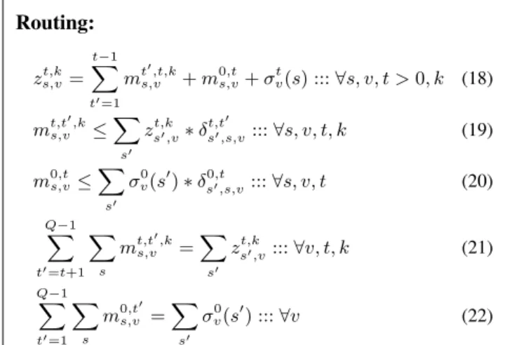
Figure 1: (a) and (d) Performance comparison of MSS and LDD. (b) and (e) Lost demand comparison of LDD for different∆
andQvalues. (c) and (f) Lost demand comparison of LDD for differentQvalues.
5 10 15 20 25 30
Number of samples 0
50 100 150 200
Lost Demand
GOAH - Hubway
(a)
5 10 15 20 25 30
Number of samples 0
200 400 600 800 1000
Lost Demand
GOAH - Capital BikeShare
(b)
5 10 15 20 25 30
Number of samples
0 2 4 6 8 10 12 14 16
Runtime(in seconds)
Hubway Capital
GOAH - Runtime
(c)
Figure 2: Performance comparison of GOAH
STREP ESOF-Rev ESOF(∆ = 10) ESON LDD GOAH
(∆ = 10, Q= 6) (∆ = 10, Q= 6) (∆ = 10, Q= 3)
Hubway(3PM) 278.32 225.95 225.93 172.11 141.16 181.67
Capital BikeShare(3PM) 1320.93 960.30 795.28 745.61 666.78 824.03
Hubway(6AM) 184.82 130.30 122.69 98.63 56.85 92.75
Capital BikeShare(6AM) 508.27 456.96 410.60 323.17 288.87 341.71
Table 5: Lost demand reduction
ESOF-Rev ESOF(∆ = 10) ESON(∆ = 10, Q= 6) LDD(∆ = 10, Q= 6) GOAH(∆ = 10, Q= 3)
Fuelcost 7.84 32.64 31.26 30.60 26.60
Revenue 431.10 422.87 461.11 488.58 441.72
Gain 423.25 390.23 429.85 457.98 415.11
Table 6: Fuel cost comparison-Hubway 3pm
Trip Duration ESOF-Rev ESOF(∆ = 10) ESON(∆ = 10, Q= 6) LDD(∆ = 10, Q= 6) GOAH(∆ = 10, Q= 3)
0-30 1166.74 1169.26 1212.17 1232.34 1205.55
30-60 93.43 91.24 102.84 112.51 97.73
60-90 11.27 11.11 11.62 12.50 11.39
>90 7.88 7.69 8.11 8.22 7.95
Number of Samples:In the first set of experiments on MSS and LDD, we experiment with different numbers of samples. Figure (1a) shows results for the Hubway dataset and Figure (1d) shows results for the Capital BikeShare dataset. The X-axis represents the number of samples and Y-X-axis represents the lost demand values. On the Hubway dataset, MSS could not compute a reasonable quality solution (the optimality gap remained at 80%) within 1 minute for more than 5 sam-ples for∆ = 5and for more than 10 samples for∆ = 10. On the Capital Bikeshare data set, for∆= 5 and a time limit of 1 minute, MSS did not find a solution of reasonable qual-ity even when only a single sample was used. On both the datasets, we observe that for LDD, lost demand reduces on increasing the number of samples, but the reduction in lost demand is less than 5% on increasing samples beyond 10.
For∆ = 5, on the Capital BikeShare, LDD could not
com-plete even 10 iterations within 1 minute and hence, the lost demand increases on increasing samples from 10 to 15. As the lost demand reduction is not significant after 10 samples and the problem also becomes complex , we use 10 samples for LDD and MSS in the next experiments.
Decision Epoch Duration(∆): In the next set of experi-ments, we fix the lookahead period for approaches to 30 minutes and experiment with different decision epoch du-ration. As∆∗Q=30 minutes, the value of Q is taken as30∆. Figure (1b) shows results on the Hubway dataset and Figure (1e) shows the results on the Capital BikeShare dataset. We fix the number of samples as 10. We only show results for LDD as MSS was not able to compute a reasonable qual-ity solution within 1 minute for 10 samples for majorqual-ity of scenarios. On both datasets, lost demand decreases on de-creasing the value of∆. This is because vehicle is allowed to make more movements and also because we are looking at demand values at smaller intervals which allows making better online decisions. On decreasing∆from 10 to 5, lost demand reduces by nearly 15% on both datasets.
Lookahead Period:For a fixed value of∆, we experiment with different lookahead period durations. We show the re-sults for∆ = 10with lookahead period between 30 minutes and 1 hour. For∆ = 15, we show the results for lookahead period between 30 minutes and 1.5 hours. Figures (1c) and (1f) show the results for differentQvalues. On increasing the look ahead period lost demand reduces for both∆values but the reduction is more with∆ = 10. With∆ = 10and
Q = 6 (i.e., lookahead period of 1 hour), the lost demand values are comparable to ∆ = 5and Q = 6(lookahead period of 30 minutes). With∆ = 10, lost demand reduces by 12% on increasingQvalue from 3 to 6. But the rate of reduction is low with higher∆ value. As the lost demand reduction provided by∆ = 10, Q= 6is comparable to lost demand reduction with∆ = 5, we use∆ = 10, Q = 6for further comparison as this involves lesser vehicle movement. GOAH Performance:We experiment with different num-ber of samples for GOAH for∆ = 10, Q = 3. In case of GOAH, along with lost demand we also compare the run-time on both datasets with different number of samples. Fig-ure (2a) and (2b) show the lost demand comparison on creasing the number of samples. On both datasets, on in-creasing samples from 5 to 15, lost demand reduces by 8%
but on increasing beyond 15 samples reduction is 2%. With 15 samples, on both datasets, GOAH obtains a runtime of less than 8 seconds (Figure (2c)). Therefore, it is possible to execute GOAH on larger bike sharing systems where it is even difficult for offline approaches to compute a solution. As described later, GOAH provides nearly 35% reduction in lost demand as compared to no repositioning strategy. Comparison Of Different Algorithms: Next, we com-pare the reduction in lost demand values obtained by dif-ferent algorithms. We compare LDD(∆ = 10, Q = 6), GOAH(∆ = 10, Q = 3) with ESOF(∆ = 10), ESOF-Rev, ESON(∆ = 10, Q = 6) and STREP on both datasets. For LDD we use 10 samples and for GOAH 15 samples. Table 5 shows the lost demand values on both datasets for 6AM and 3PM. As we can see on both datasets, LDD reduces the lost demand by nearly 50% as compared to STREP and provides 20% gain over ESOF and ESON. The lost demand reduction by GOAH is comparable to ESOF and ESON but it provides improvement in runtime which is the main advantage of us-ing it against other approaches.
Comparison Of Fuel cost:Finally we compare the fuel cost incurred by different algorithms. We use the cost of diesel as 1.5 USD per litre and assume that the vehicle can travel 12 kilometer with 1 litre of fuel. Here, we show the results on the Hubway dataset at 3pm. We obtained similar results on the other dataset. We then compare the fuel cost incurreed by various algorithms in Table 6. As we do not consider the fuel cost in our objective, fuel cost of our algorithm is nearly 4 times the cost of fuel consumed by ESOF-Rev. We also compute the revenue obtained by bike sharing company by using the standard price model where only rides greater than 30 minutes are charged6. The revenue increase compensates
for the additional fuel cost in case of LDD. With GOAH, both the fuel cost and revenue gain are less than LDD. Over-all gain provided by GOAH is less than ESOF-Rev.
As the rides having travel time less than 30 minutes are included in the subscription cost, we also compare the num-ber of bikes hired for different trip duration by various algo-rithms (Table 7). Once again, LDD provides the best results. As the major percentage of bikes are hired for duration 0-30 minutes, the lost demand reduction of these rides does not directly contribute to daily revenue. But this reduction will help in increasing the number of new subscribers which will provide additional profit to bike sharing companies.
7
Conclusion
We develop a multi-stage stochastic optimization formula-tion for computing online reposiformula-tiong and routing policy for vehicles in bike sharing systems. We also provide a la-grangian based decomposition and greedy based heuristic approach to efficiently reduce lost demand for large scale bike sharing systems. In future, this work can be extended to compute online policies which can simultaneously and ef-ficiently optimize reduction of lost demand and fuel cost of vehicles. Another possible direction is to include uncertainty in travel time of vehicles, so as to compute robust policies.
6
8
Acknowledgements
This work was partially supported by the Singapore National Research Foundation through the Singapore-MIT Alliance for Research and Technology (SMART) Centre for Future Urban Mobility (FM).
References
Chemla, D.; Meunier, F.; and Calvo, R. W. 2013. Bike shar-ing systems: Solvshar-ing the static rebalancshar-ing problem. Dis-crete Optimization10(2):120–146.
Contardo, C.; Morency, C.; and Rousseau, L.-M. 2012. Balancing a dynamic public bike-sharing system, volume 4. Cirrelt.
Fisher, M. L. 1985. An applications oriented guide to la-grangian relaxation.Interfaces15(2):10–21.
Ghosh, S., and Varakantham, P. 2017. Incentivising the use of bike trailers for dynamic repositioning in bike sharing systems. InInternational Conference on Automated Plan-ning and Scheduling (ICAPS).
Ghosh, S.; Varakantham, P.; Adulyasak, Y.; and Jaillet, P. 2015. Dynamic redeployment to counter congestion or star-vation in vehicle sharing systems. InInternational Confer-ence on Automated Planning and Scheduling (ICAPS). Ghosh, S.; Varakantham, P.; Adulyasak, Y.; and Jaillet, P. 2017. Dynamic repositioning to reduce lost demand in bike sharing systems. Journal of Artificial Intelligence Research 58:387–430.
Ghosh, S.; Trick, M.; and Varakantham, P. 2016. Robust repositioning to counter unpredictable demand in bike shar-ing systems. InInternational Joint Conference on Artificial Intelligence (IJCAI).
Lowalekar, M.; Varakantham, P.; and Jaillet, P. 2016. On-line spatio-temporal matching in stochastic and dynamic do-mains. InAAAI Conference on Artificial Intelligence (AAAI).
Mercier, L., and Van Hentenryck, P. 2007. Performance analysis of online anticipatory algorithms for large multi-stage stochastic integer programs. InIJCAI, 1979–1984.
Pfrommer, J.; Warrington, J.; Schildbach, G.; and Morari, M. 2014. Dynamic vehicle redistribution and online price incentives in shared mobility systems. IEEE Transactions on Intelligent Transportation Systems15(4):1567–1578.
Raviv, T.; Tzur, M.; and Forma, I. A. 2013. Static repo-sitioning in a bike-sharing system: models and solution ap-proaches. EURO Journal on Transportation and Logistics 2(3):187–229.
Schuijbroek, J.; Hampshire, R.; and van Hoeve, W.-J. 2017. Inventory rebalancing and vehicle routing in bike shar-ing systems. European Journal of Operational Research 257(3):992–1004.
Shu, J.; Chou, M. C.; Liu, Q.; Teo, C.-P.; and Wang, I.-L. 2013. Models for effective deployment and redistribution of bicycles within public bicycle-sharing systems. Operations Research61(6):1346–1359.
Zhang, G.; Smilowitz, K.; and Erera, A. 2011. Dy-namic planning for urban drayage operations. Transporta-tion Research Part E: Logistics and TransportaTransporta-tion Review 47(5):764–777.