Intermediate Microeconomics Lecture Notes – Spring 2012
Michael Malcolm
Unit 1: Introductory Material
1.1: Quantitative supply and demand models
1.2: Calculus review
1.3: Elasticities
Unit 2: Consumer Choice Model (graphical)
2.1: Model setup
2.2: Consumer optimization
2.3: Foundations of demand
Unit 3: Consumer Choice Model (mathematical)
3.1: Demand functions
3.2: Slutsky equation and other relationships
3.3: Duality
3.4: Perfect Complements and Perfect Substitutes
3.5: Revealed preference
Unit 4: Applications and Extensions of the Consumer Choice Model
4.1: Labor/leisure choice
4.2: Intertemporal choice
4.3: Choice over uncertainty
4.4: Consumer welfare
Unit 5: Firm Theory
5.1: Production
5.2: Costs
Unit 6: General Equilibrium
6.1: Exchange economies (graphical)
6.2: Exchange economies (mathematical)
Unit 7: Game Theory
7.1: Preliminaries
7.2: Simultaneous games
7.3: Sequential games
Unit 8: Market Failure
8.1: Externalities
8.2: Public goods
8.3: Adverse selection and signaling
Unit 1.1: Quantitative Supply and Demand Analysis
Michael Malcolm
June 18, 2011
1
Quantitative Models in Economics
There are basically three ways to express economic ideas: verbally, graphically and mathematically. Principles-level economics courses typically stress verbal and graphical reasoning. In this class, while we will deal with all three to some extent, the emphasis will be on mathematical reasoning and presentation of economic ideas. Most economic models that you have studied at the principles level can be presented quantitatively. Indeed, the main topics of this course are similar to those that are covered in a principles of microeconomics course. The difference is that we will approach topics mathematically. Many students eventually find the mathematical approach easier and more straightforward.
For better or for worse, mathematics has become the language of economics, and you need to be com-fortable with quantitative reasoning. On a philosophical level, it may be true that mathematics is limiting in a sense, but it certainly is the best way to be precise in your reasoning. It is easy to be misled by verbal or graphical arguments, but properly done math does not lie.
With this in mind, let us begin with a simple supply and demand model. This section is just to give you a feel for how to work with the model mathematically, and to see how results familiar from principles courses can be shown quantitatively.
2
Expressing Supply and Demand Quantitatively
Quantity demanded and quantity supplied are both functions of the price. Quantity demanded falls as price rises, so we say that quantity demanded is a decreasing function of the price. Quantity supplied rises as price rises, so we say that quantity supplied is anincreasing function of the price.
Where P denotes the market price, we will let QD and QS stand for quantity demanded and quantity supplied, respectively. In the example we will work with:
QD= 4000−400P QS =−2400 + 1200P
3
Equilibrium
Market equilibrium occurs where supply and demand are equal:
QD=QS
4000−400P =−2400 + 1200P 6400 = 1600P
Figure 1: Supply and Demand Sketch
Then substitute this back to either the supply or the demand curve to findQ= 2400. So the equilibrium price in this market isP = 4 with the equilibrium quantityQ= 2400.
4
Graphical
In the typical supply and demand diagram, the price is measured on the vertical axis and the quantity is measured on the horizontal axis. Therefore, we need to solve the supply and demand equations forP to get them into slope-intercept form to facilitate graphing. For the demand curve:
QD= 4000−400P 400P = 4000−QD
P = 10− 1 400Q
D
So the demand curve has an intercept of 10 and a slope of − 1 400. For the supply curve:
QS =−2400 + 1200P 1200P = 2400 +QS
P = 2 + 1 1200Q
S
So the supply curve has an intercept of 2 and a slope of 12001 . Notice that the demand curve is steeper than the supply curve. Sketching the supply and demand curves, notice that they cross at the equilibrium price and quantity,P = 4 andQ= 2400. See figure 1 for a sketch of the diagram.
5
Regulated Prices
QD= 4000−400P = 4000−400(3) = 2800 QS=−2400 + 1200P =−2400 + 1200(3) = 1200
Buyers want to buy 2800 units, but sellers are only willing to sell 1200 units. As a result, there are Q= 1200 units exchanged in the market, and there is ashortage ofQD−QS = 1600 units.
Aprice floor is a regulated minimum price, and therefore must be setabove the market price in order to have an impact on the market. For example, suppose that the government sets the price in this market at P = 6. In this case:
QD= 4000−400P = 4000−400(6) = 1600 QS=−2400 + 1200P =−2400 + 1200(6) = 4800
Sellers want to sell 4800 units, but buyers are only willing to buy 1600 units. As a result, there are Q= 1600 units exchanged, and there is asurplus ofQS−QD= 3200 units.
6
Excise Taxes
Suppose that the government charges the seller a tax of $2 for each unit that is exchanged. The normal way to work with this is to letP continue to stand for the exchange price that the buyer pays to the seller. What this means is that the buyer paysP, but the seller receives onlyP−2 since the seller has to pay $2 to the government for each unit sold. We need to modify the supply and demand curves. The demand curve is unchanged since the buyer still paysP, but the supply curve needs to be adjusted to reflect the fact that the seller only receivesP−2.
QD= 4000−400P
QS =−2400 + 1200(P−2)
We find equilibrium by setting the demand curve equal to the modified supply curve:
QD=QS
4000−400P=−2400 + 1200(P−2) 4000−400P=−2400 + 1200P−2400
8800 = 1600P ⇒P= 5.5
Then substitute back to either the demand curve or modified supply curve to findQ= 1800.
Notice in this case that the buyer pays P= 5.5, but the seller receives anet price (orafter-tax price) of only $3.50 after paying the $2 tax.
Since the original price is $4, but the buyer now pays $5.50, this means that the buyer is paying $1.50 (or 75%) of the tax.
The seller receives $3.50; comparing to the pre-tax price of $4 implies that the seller pays $0.50 (or 25%) of the tax.
7
Excise Taxes Charged to Buyers
Suppose now that we force thebuyer, rather than the seller, to pay a $2 tax for each unit exchanged. Again, we let P designate the exchange price that the buyer actually pays to the seller. In this case, the supply curve is unchanged since the seller receivesP. However, the buyer actually paysP + 2 since he has to pay P, and also an additional $2 to the government. The relevant equations are, therefore:
QD= 4000−400(P+ 2) QS=−2400 + 1200P Solving for the new equilibrium:
QD=QS
4000−400(P+ 2) =−2400 + 1200P 4000−400P−800 =−2400 + 1200P
5600 = 1600P ⇒P = 3.5
Substituting back to either curve gives the equilibrium quantity Q = 1800 (the same as the previous case).
In this case, the seller receives $3.50, but the buyer pays a net price of $5.50 since he also has to pay a $2 tax to the government. The buyer pays $1.50 more than the original equilibrium price of $4, and the seller receives $0.50 less; that is, the economic incidence of the $2 tax falls 75% on the buyer and 25% on the seller.
But notice that this is the same as what we obtained in the previous section! The economic incidence of the tax (75% to the buyer and 25% to the seller in this case) is the same regardless of whether the tax is charged to the buyer or to the seller. In terms of the actual impact on the market, it makes no difference whatsoever. This is an example of a result that is cumbersome to show graphically, and may be difficult to understand verbally, but is quite straightforward mathematically.
8
VAT (sales) Taxes
Instead of a fixed excise tax, suppose that the seller is required to pay a VAT tax equal to 20% of the sale price of the product. Since P is the exchange price that the buyer pays to the seller, the demand curve is unchanged. However, the seller receives only 0.8P since 20% of the exchange price is paid to the government. The supply and demand equations for this case are:
QD= 4000−400P QS=−2400 + 1200(0.8P) Solving for the new equilibrium:
QD=QS
4000−400P =−2400 + 1200(0.8P) 4000−400P =−2400 + 960P
Substituting into either curve gives the equilibrium quantityQ= 2118.
Notice that the buyer pays $4.71, but the seller is required to turn over 20% of this to the government, so the seller receives a net price of only 0.8(4.71) = 3.76. This difference 4.71−3.76 = 0.95 is known as the tax wedge. The buyer pays $4.71 instead of $4, meaning that he pays $0.71 of the tax wedge, with the seller paying $3.76 of the tax wedge. Like before, this tax wedge is distributed (modulo rounding error) 75% to the buyer and 25% to the seller.
Notice that a 20% excise tax charged to the buyer would be similar to the above. In this case, againP is the exchange price paid to the seller, so the supply curve remains unchanged. However, the price in the demand curve is raised to 1.2P to reflect that the buyer has to pay an additional 20% over the exchange price as a tax.
9
Summary of Taxes
To summarize the discussion above regarding the incorporation of taxes into the basic supply and demand model:
• Excise tax of $t charged to seller: ChangeP toP−t in the supply equation • Excise tax of $t charged to buyer: ChangeP toP+t in the demand equation • VAT tax of 100·τ% charged to seller: ChangeP to (1−τ)P in the supply equation • VAT tax of 100·τ% charged to buyer: ChangeP to (1 +τ)P in the demand equation
Unit 1.2: Calculus Review
Michael Malcolm
June 18, 2011
1
Slope and Derivatives
The idea of slope is familiar from elementary algebra courses. The slopemof a function tells us how ”steep” the function is. It is the change in Y for each one-unit change in X. In other words, the ratio of the change in Y to the change in X:
m= ∆Y ∆X For example, consider the function in figure 1.
Calculated between points A and B, the slope of the function is 3:
m= ∆Y ∆X =
5−2 3−2 =
3 1 = 3 Or between points B and C:
m= ∆Y ∆X =
8−5 4−3 =
3 1 = 3
For a straight line (linear function), the slope is the same anywhere along the line. However, this is not true for all functions. For example, consider the function in figure 2.
We cannot define a single slope for the function in figure 2, because it changes as we move along the function. For example, the function slopes upwards at point A, downwards and point C and is flat at point B.
What wecan do is to find the slope at any particular point. Geometrically, the way we do this is to draw a line tangent to the graph at any given point; the slope of this tangent line then gives us the slope of the functionat that point.
Figure 2: Nonlinear function
Figure 3: Nonlinear function with tangent lines
For example in figure 3, the tangent line drawn at point A is positively sloped, so we can say that the function has a positive slope at point A. At point B, the tangent line is flat, so we can say that the function has a slope of 0 at point B.
The derivative of a function is the slope at any point. Naturally, for a straight line, the derivative is constant. For the straight line in figure 1, the derivative is equal to 3 everywhere along that line. However, the derivative of the function in figure 2 is different at different points. It is positive at point A, negative at point C and zero at point B.
We can plug in to the derivative function to find the slope of a function at any given point. For a function f(x), we denote the derivative of the function as dxdf. For example, for the functionf(x) =x2, the derivative is dxdf = 2x.
See the diagram in figure 4. Using the formula for the derivative, the slope of the function at x= 12 is equal to dxdf = 2(12) = 1. The slope of the function at x= 1 is dxdf = 2(1) = 2. The function is twice as steep here. If we move tox= 2, the function is even steeper, with a slope of dxdf = 2(2) = 4.
2
Rules for Calculating Derivatives
There are straightforward rules for calculating the derivatives of the functions we will work with in this class. • Forf(x) =xn, the derivative is df
dx =nx n−1
– Example: Forf(x) =x3, the derivative is dxdf = 3x2 – Example: For Forf(x) =x34, the derivative is df
dx = 3 4x
−1 4 • Forf(x) =ag(x), whereais any constant, the derivative is dxdf =adxdg • Forf(x) =axn, the derivative is dxdf =anxn−1
– Example: Forf(x) = 4x6, the derivative is df
dx = 4 6x 5
= 24x5 – Example: Forf(x) = 2x−3, the derivative is dxdf = 2 −3x−4
=−6x−4 – Example: Forf(x) = 4x, the derivative is dxdf = 4 1x0
= 4 • Forf(x) = ln(x), the derivative is dxdf =x1
– Example: Forf(x) = ln(x2), recall that the function can be written asf(x) = 2 ln(x). Then the derivative is dfdx= 2∗ 1
x= 2 x
• Forf(x) =g(x) +h(x), the derivative is dxdf = dgdx+dh dx
– Example: Forf(x) =x4+ 3x2+ ln(x), the derivative is df dx = 4x
3+ 6x+1 x • Forf(x) =g(x)h(x), the derivative is dxdf =dxdgh(x) +dh
dxg(x) – Example: Forf(x) =x2ln(x), the derivative is df
dx = (2x) (ln(x)) + 1 x
(x2) = 2xln(x) +x • Forf(x) = g(x)h(x), the derivative is dxdf =
dg
dxh(x)+dhdxg(x) h(x)2
– Example: Forf(x) = 1+2xx , the derivative is dfdx= 1(1+2x)−2(x)(1+2x)2 = 1 (1+2x)2 • Forf(x) =g(h(x)), the derivative is dxdf = dg(h(x))dx dh
dx – Example: Forf(x) = x2+x34, the derivative is df
dx = 4 x
2+x33 2x+ 3x2 – Example: Forf(x) = ln(x2), the derivative is df
dx = 1 x2
(2x) = 2 x Here are a few examples to illustrate combining the rules.
• For f(x) = √x+√1
x, first rewrite the function as f(x) = x 1 2 +x−
1
2, then the derivative is df dx = 1
2x −1
2 +−1 2x
−3 2
• Forf(x) =x(10−4x)−x2, first rewrite the function asf(x) = 10x−4x2−x2= 10x−5x2. Then the derivative is dfdx = 10−10x.
• Forf(x) = ln(x3+ 4), the derivative is dxdf =x31+4
3x2= x3x3+42 • Forf(x) =√x3+ 4, the derivative is df
dx = 1 2 x
2+ 4
3
Partial Derivatives
For a function of more than one variable, we can calculate thepartial derivative with respect to a single one of those variables. This is generally denoted with a ”crooked” derivative sign. For example, for a function f(x, y) that depends on the variablesxandy, we denote the partial derivative with respect toxas ∂f∂x.
To calculate a partial derivative, simply differentiate with respect to the given variable and treat all other variables as constant. For example, consider the function f(x, y) = 3x+ 4x3y+ 2y+ 16xy2. To find the partial derivative with respect tox, differentiate this function with respect to x, while treatingy and any function ofy as a constant:
∂f
∂x = 3 + 4y(3x
2) + 0 + 16y2 = 3 + 12x2y+ 16y2
We can also calculate the partial derivative with respect toyby differentiating with respect toy, treating xas a constant:
∂f
∂y = 0 + 4x
3+ 2 + 16x(2y) = 4x3+ 2 + 32xy Here are some more examples of partial differentiation.
• Forf(x, y) = 2x+ 3y2+xy, the partial derivative with respect toxis ∂f
∂x = 2 +y • Forf(x, y) = 4x3y2+13x+12y−4xy2, the partial derivative with respect toxis ∂f
∂x = 12x
2y2+13−4y2 • Forf(x, y) =x13y23, the partial derivative with respect toxis ∂f
∂x = 1 3x
−2 3y23 • For f(x, y) = ln x2y3
, first rewrite asf(x) = ln x2
+ ln y3
= 2 ln(x) + 3 ln(y). Then the partial derivative with respect toxis ∂f∂x =x2
• Forf(x, y) =√x+√y, first rewrite asf(x) =x12 +y 1
2. Then the partial derivative with respect tox is ∂f∂x = 12x−12 = 1
2√x
• Forf(x, y) =x+yxy , the partial derivative with respect toxis ∂f∂x = y(x+y)−xy(x+y)2 =
xy+y2−xy (x+y)2 =
y2 (x+y)2
4
Optimization
How does any of this help us in economics? At its core, microeconomics is about solving optimization prob-lems: firms maximize profit, governments try to minimize deadweight loss of taxation, consumers maximize happiness given a fixed level of income, etc...
Why calculus is helpful to us is that the solution to many optimization problems can be expressed in terms of derivatives. For example, looking back at figure 3, we can see that the maximum value of the function is at point B, which is precisely where the derivative is equal to zero. To find the maximum value of this function, we would simply find the value ofxwhere the derivative is equal to zero.
Is this always the recipe for finding the maximum value of functions? Not necessarily. To see what can go wrong, consider the examples below.
Figure 5: Finding a minimum rather than a maximum
Figure 6: Multiple local maxima
• We might be finding a local maximum rather than the global maximum. For example, in figure 6, the derivative of the function at points A and B is equal to 0, but these are onlylocal maxima of the function. For the function pictured, only point C is aglobal maximum.
• The maximum value could occur on the boundary of the set. For example, consider figure 7. If we are interested in finding the maximum value of the function over the seta6x6b, then it is clearly on the border, atx=b. However, the derivative is not equal to 0 at this point (butis equal to zero at two points in the interior of the set that are not the maximum). In general, derivative characterizations only work for interior solutions, not for boundary solutions.
• Some functions have no maximum at all. For example,f(x) =x2 grows without bound asxincreases, and therefore has no maximum.
The rules for determining whether setting the derivative equal to zero will locate the maximum, particu-larly in multivariate functions, can get complex and tricky. This topic is covered in mathematical economics or multivariate calculus classes, and we will not cover it here in any detail. However, using derivatives is the cleanest, easiest way to characterize solutions to optimization problems. We will not deal with these
technicalities in this class. If I give you a function to maximize, you can assume that the maximum exists and that the derivative characterization will work properly.
Here are some examples of maximization problems solved using derivatives. • Find the maximum value of the functionf(x) = 12x−3x2+ 12.
Setting the derivative equal to zero.
df
dx = 12−6x= 0 12 = 6x ⇒x= 2
This function is maximized when x= 2. Then the maximum value of the function isf(x) = 12(2)− 3(2)2+ 12 = 24. We say that x = 2 is the maximizer of the function and that f(2) = 24 is the maximum of the function.
• A firms profit is Π(Q) = 90Q−Q2, whereQis the amount of output the firm produces. Find the value ofQthat maximizes the firm’s profit.
Again, setting the derivative equal to zero.
dΠ
dx = 90−2Q= 0 2Q= 90 ⇒Q= 45
This firm maximizes profit by producingQ= 45 units of output. Notice that the firm earns $ 2025 of profit in this case.
• The total profit earned by a firm depends onq1 andq2, which represent the output produced at plant 1 and plant 2, respectively. The profit function is Π(q1, q2) = 100q1+ 100q2−3q21−3q22+ 2q1q2. What values ofq1 andq2 maximize the firm’s profit?
We solve this by calculating both partial derivatives and setting them equal to zero.
∂Π ∂q1
= 100−6q1+ 2q2= 0 ∂Π
∂q2 = 100−6q2+ 2q1= 0
Unit 1.3: Elasticities
Michael Malcolm
June 18, 2011
1
Price Elasticity of Demand
Elasticities measure the responsiveness of one variable to a change in another variable. Probably the most well-known example in economics isprice elasticity of demand, which measures the percent change in quantity demanded for a product resulting from a 1% increase in the price of the product. Price elasticities are denoted withε.
As such, price elasticities are almost alwaysnegative numbers: quantity demanded falls as price rises, so a 1% increase in the price of a product causes a negative percent change in demand for the product.
Recall the various ranges of elasticities.
• Perfectly inelastic: ε= 0
• Inelastic: −1< ε <0
• Unit Elastic: ε=−1
• Elastic: −∞< ε <−1
• Perfectly elastic: ε=−∞
Goods that people can’t live without and goods without many substitutes tend to be more inelastic, meaning that quantity demanded doesn’t decline much when price rises. For example, for tobacco products,
ε = −0.45. However, for foreign travel ε = −4, meaning that consumers substantially decrease their foreign travel when the price rises. The time horizon also matters; gasoline is very inelastic in the short-run (ε = −0.2) since consumers don’t change their cars or driving habits immediately in response to a price change. However, over the long run, gas is more elastic (ε =−0.7) after consumers have had a chance to change their vehicles or their driving habits.
2
Midpoint Method
Calculation of elasticities in principles courses typically uses the midpoint method. Here is a simple example. At $10, consumers buy 400 t-shirts from a vendor, but when the vendor raises his price to $15, consumers buy only 300 t-shirts. Now, elasticity is the percentage change in quantity relative to the percentage change in price.
ε= %∆Q
D
%∆P
ε=%∆Q D %∆P = 300−400 350 15−10
12.5
=−0.715
3
Point Elasticity
The midpoint method is useful for finding an approximate elasticity over a range. But suppose instead that you wanted to calculate anexact elasticity at apoint. To motivate this definition, suppose again that consumers purchaseQ1 at priceP1, butQ2 at priceP2. Starting with the midpoint formula, the elasticity is then:
ε= %∆Q %∆P =
Q2−Q1
Q
P2−P1 P
The difficulty comes about in what QandP to use for the denominators. The midpoint method would have us take the average of the two observations. However, if Q1 and Q2 are very close to each other, infinitesimally close, then it doesn’t much matter which one we use for the calculation. The same thing applies to the prices. Let us manipulate the expression above, keeping this in mind:
ε=
Q
2−Q1 Q
P2−P1 P
=
Q2−Q1 P2−P1
P Q = ∆Q ∆P P Q
But ∆∆QP is just the slope of the line, which defined at a single point is precisely the derivative ∂Q∂P. This gives us the proper formula for price elasticity.
ε= ∂Q ∂P P Q
4
Example: Linear Demand
Consider the demand curve
Q= 100−2P
Figure 1: Elasticity along a linear demand curve ε= ∂Q ∂P P Q
= (−2)
40
20
=−4
At a price ofP = 5 (with corresponding quantityQ= 90), the elasticity is
ε= ∂Q ∂P P Q
= (−2)
5 90
=−0.11
Observe that the elasticity is different at different points along the demand curve. See figure 1 for a sketch.
At what price does unit elasticity occur? We can simply substituteε=−1 and solve for the price.
ε= ∂Q ∂P P Q
−1 = (−2)
P Q
−1 = (−2)
P
100−2P
−100 + 2P =−2P ⇒P = 25
5
Example: Constant elasticity demand curve
Consider the demand curve
Q= 100P−2
Let us find the elasticity atP = 5 (whereQ= 4).
ε= ∂Q ∂P P Q
= −2∗100P−3 5
4
= −2∗100∗5−3
5
4
=−2
Let us again find the elasticity atP = 2 (whereQ= 25).
ε= ∂Q ∂P P Q
= −2∗100P−3
2 25
= −2∗100∗2−3
2
25
=−2
It turns out that the price elasticity isε=−2 atany point along this demand curve. In fact, we can generally consider any demand curve with the following form.
Q=APb
Calculating the price elasticity along this demand curve:
ε= ∂Q ∂P P Q
= bAPb−1 P Apb = bAp b Apb =b
6
Other Elasticities
Other elasticities can be defined along the same lines. For example, letting Y designate income and Q
designate quantity demanded, then theincome elasticity of demand is defined as
ξ= ∂Q ∂Y Y Q
For example, suppose that demand for a product depends on income Y and the price of the productP
according to the following formula
Q= 1 4
Y P
Notice that this formula makes sense as a demand curve. Demand rises as Y rises but falls as P rises. Now, to calculate the income elasticity of demand:
ξ= ∂Q ∂Y Y Q = 1 4P ·
Y
Y
4P
= 1
For this particular demand function, the income elasticity is always equal to 1.
The cross-price elasticity of demand is the percentage change in the demand for product A when the price of product B rises by 1%. It is calculated as follows:
εA,B=
∂Q A ∂PB PB QA
Supply elasticity is the percentage change in quantity supplied resulting from a 1% increase in price.
η= ∂QS ∂P P QS
7
Application: Tax Incidence
At the principles level, you learned that the economic incidence of a tax depends on the elasticities of demand and supply. For markets with a relatively inelastic demand (and more elastic supply), the majority of the tax burden will fall on buyers. This makes good economic sense; if buyers do not reduce their purchases much as a result of price increases, then the seller can easily pass most of the tax on to the buyer. For markets where supply is more inelastic than demand, the majority of the tax burden falls on sellers.
To be precise, whenεis the price elasticity of demand andη is the price elasticity of supply, the share of the tax paid by thebuyer is
sharebuyer=
For example, in a market where ε =−0.1 and η = 2, the proportion of the tax burden borne by the buyer issharebuyer=2+02.1 = 0.952. The buyer pays the majority of the tax in this market since demand is
more inelastic than supply.
However, in a market where ε=−2 and η= 1, the proportion of the tax burden borne by the buyer is
sharebuyer= 1+21 = 0.33. The buyer pays only 1
3 of the tax in this case, with the seller paying the other 2 3.
Unit 2.1: Consumer Theory (Graphical Presentation): Model Setup
Michael Malcolm
June 18, 2011
1
Consumer Choice Problem
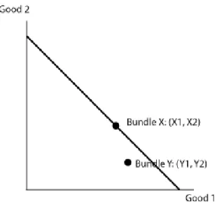
A consumer chooses among many different goods – which goods to buy and how much to buy of each good. In order to simplify the problem (particularly to make graphical analysis possible), we often reduce the problem to only two goods over which the consumer can choose. Abundle is some combination of the two goods.
We can depict different bundles as different points on a diagram, as in figure 1. Throughout, we will use fish and apples as our two goods.
For example, the bundle containing 7 fish and 4 apples is represented by point A. The bundle containing 4 fish and 9 apples is represented by point B. The bundle containing no fish and 5 apples is represented by point C. Each point on the graph is a different bundle.
Note that what’s measured on the axes of this graph are justquantities of the two goods. Not prices and not dollar amounts – just different quantities.
2
The Budget Constraint
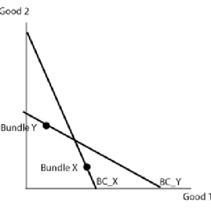
The consumer can’t just choose any bundle he wants to choose. The bundle has to be affordable. Thebudget constraint is the set of all bundles that use up the consumer’s income, given the prices of the two goods.
For example, suppose that the price of a fish is $3, the price of an apple is $3, and that the consumer has $12 of income to spend. The line in Figure 2 shows all of the bundles that the consumer can choose in order to spend his $12.
As shown in figure 2, one choice is to buy 4 fish and no apples. At $3 per fish, this spends the consumer’s $12. Alternatively, the consumer could choose to buy 4 apples and no fish; this also spends his $12. There are other possibilities, too. For example, the bundle with 2 fish and 2 apples also costs $12.
A simple, linear budget constraint is easy to draw. Just figure out the two endpoints: How many fish could the consumer buy if he spentall his money on fish? How many apples could he buy if he spendall his money on apples? Then draw a straight line connecting these endpoints.
Budget lines can get more complicated, for example when stores follow a pricing strategy that leads to a different per-unit price depending upon the number of units bought (e.g. products with a quantity discount). Also, public policies sometimes create strange-looking budget constraints. You will study these more in labor economics or public economics classes. In this class, we will focus on the simple linear budget constraint, which is enough to understand the basic consumer choice model.
Theprice ratio is the price of the good measured on the X axis divided by the price of the good measured on the Y axis. The slope of the budget line is the negative of the price ratio:
slopebudget=−PX
Figure 1: Different Bundles
Figure 3: An increase in the price of fish
In this case, the price of fish is 3 and the price of apples is 3. This means that the price ratio is 1, and so the slope of the budget line is
slopebudget=−PX
PY =−3
3 =−1
The price ratio represents the number of units of good Y that the consumer must give up in order to obtain one more unit of good X. For example, when apples and fish each cost $3, the consumer gives up one apple (the good on the Y axis) in order to obtain one more fish (the good on the X axis).
Suppose now that the price of fish increases to $6, with the price of an apple remaining at $3. If the consumer spends all his $12 income on fish, he can only afford 2 fish. If he spends all his income on apples, again he can afford 4 apples. The new budget constraint is shown in figure 3.
Notice that a price increase pivots the budget lineinwards along the axis measuring the good whose price rose. Intuitively, a price increase means that the consumer can now afford less of the good, so the budget line pivots inwards. Conversely, a decline in the price of fish means that the consumer can afford more fish, pivoting the budget lineoutwards.
With the new prices, the price ratio is now:
PX PY
= 6 3 = 2
Geometrically, the budget line is twice as steep, with a slope of −PX
PY =−2 . Since the price ratio is 2, this means that the consumer now has to give up 2 apples in order to obtain one more fish. This makes intuitive sense since fish are now twice as expensive as apples.
Now suppose that both the price of fish and apples remained at $3, as before, but that the consumer’s income increases from $12 to $15. In this case, the consumer can now afford 5 fish if he spends all his money on fish, and 5 apples if he spends all his money on apples. The new budget line is shown in figure 4.
As shown, an increase in income causes a parallel shift of the budget constraint. Intuitively, an increase in income increases the amount of both goods that the consumer can afford. The slope of the new budget line is the same as the slope of the original budget line since the price ratio did not change. Conversely, a decline in income shifts the budget line parallel inwards.
Figure 4: An increase in income
Figure 5: Set of affordable bundles
Anaffordable bundleis any bundle that the consumer can afford, given his income and the prices of the goods. The set of all affordable bundles includes the bundles on the budget line and all bundles inside the budget line. Bundles on the budget line use all of the consumer’s income. Bundles inside the budget line are affordable but do not use up all of the consumer’s income. The set of affordable bundles is shown in figure 5.
3
Indifference Curves
Having dealt with what a consumer is able to buy, we will now deal with what a consumer wants to buy. An indifference curve represents various bundles that all make a consumer equally well-off. That is, the consumer likes every bundle on an indifference curve equally well.
Figure 6: Indifference Curve
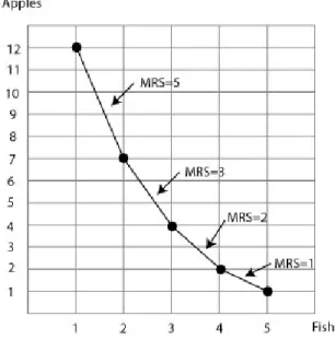
The marginal rate of substitution (MRS) is the amount of good Y that the consumer is willing to give up in order to obtain one more unit of good X. In this case, the MRS is 5 since the consumer was willing to give up 5 apples in order to obtain one more fish. Graphically, the MRS is just the negative of the slope of the indifference curve.
Now, once the consumer already has 2 fish and 7 apples, it is unlikely that the consumer would be willing to give up another 5 apples in exchange for a third fish. Since the consumer already has more fish (and fewer apples), an additional fish is not as valuable. Let us say that the consumer would be willing to give up only 3 apples to obtain another fish. Therefore, another bundle on the indifference curve is the bundle containing 3 fish and 4 apples. See figure 7. The marginal rate of substitution is 3 over this interval.
Now, when the consumer already has 3 fish (and 4 apples), he might only be willing to give up 2 apples to obtain another fish. So, another point on the indifference curve is the bundle containing 4 fish and 2 apples. The MRS is 2 over this interval.
Once the consumer already has 4 fish (and 2 apples) he might only be willing to give up 1 apple to obtain another fish. So, another point on the indifference curve is the bundle containing 5 fish and 1 apple. The MRS is one over this interval. Figure 8 diagrams out all the points we have obtained on this indifference curve.
To reiterate, in figure 8, every bundle on this curve leaves the consumer equally well off. The consumer likes every one of these bundles equally well. This is the definition of an indifference curve.
Notice that the marginal rate of substitution is not constant along the indifference curve. In fact, indifference curves typically obey the law of diminishing marginal rate of substitution. As a consumer obtains more of good X (fish), he is willing to give up fewer units of good Y (apples) in order to obtain an additional unit of good X. This makes good intuitive sense. If you have very few fish, you’d probably give up a lot of your apples to obtain another one. However, if you already have a lot of fish, you’re not willing to give up so many apples to get another one.
Graphically, what this means is that MRS declines as we move rightwards along an indifference curve – the curve flattens out as we move rightwards. This property is what gives indifference curves their characteristic convex shape shown in figure 9.
Figure 7: Indifference Curve with additional point
Figure 9: Typical indifference curve
Figure 10: Indifference Map
– the consumer is not willing to give up very many apples to obtain another fish; the indifference curve is flatter.
To reiterate one more time, every point on an indifference curve leaves the consumer equally well off.
4
Indifference Maps
It is clearly possible to draw more than one indifference curve. Anindifference mapshows multiple indiffer-ence curves. See figure 10.
5
Properties of Consumer Preferences
There are five properties that consumer preferences (represented by indifference curves) typically obey. 1. Preferences are complete. This means that a consumer is able to rank any two bundles. In other
words, for any two bundles that I name A and B, the consumer is able to tell me that he prefers A, prefers B, or likes both the same. Geometrically, this property means that we are able to draw indifference curves. If a consumer was unable to say which of two bundles he preferred, it would be impossible to represent his preferences over these bundles.
2. Preferences are transitive. This means that if a consumer prefers bundle A to bundle B and the consumer prefers bundle B to bundle C, then the consumer must prefer bundle A to bundle C. For example, if I prefer pizza to ice cream, but like ice cream better than carrots, then I must like pizza more than carrots. Geometrically, transitive preferences imply that indifference curves cannot cross. 3. Preferences are continuous. This means that if a consumer prefers bundle A to bundle B, and if
bundle C is only infinitesimally far away from bundle A, then the consumer also prefers bundle C to bundle B. What this rules out is sudden changes in preference patterns resulting from tiny changes. Geometrically, this means that indifference curves can be represented by continuous functions without breaks.
4. Preferences are monotonic. Another way to state this is ”more is better”. This just means that, starting with bundle A, if bundle B contains more of either good, then the consumer would prefer bundle B to bundle A. In other words, the commodities are ”good” and not ”bad”. Preferences over dirty cat litter are not monotonic, since a consumer would prefer to have less dirty cat litter. Geometrically, this means two things. First, higher indifference curves (containing more of both goods) are preferred to lower indifference curves. Second, indifference curves slope downwards – the consumer likes good X, and is willing to give up some good Y in order to obtain more.
5. Preferences areconvex. This is a way of saying that preferences satisfy the law of diminishing marginal rate of substitution. Geometrically, this means that indifference curves are convex to the origin – the MRS is high initially and then falls as the consumer obtains more of good X.
Unit 2.2: Consumer Theory (Graphical Presentation): Consumer
Optimization
Michael Malcolm
June 18, 2011
1
Finding the Optimal Bundle
Theoptimal bundle is the affordable bundle that leaves the consumer the best off. If preferences are well-behaved, then the optimal bundle is the bundle on the budget constraint that puts the consumer on the highest possible indifference curve.
Illustrating this on a diagram, figure 1 shows a budget line and several different indifference curves. In figure 1, bundle A is the optimal bundle. It puts the consumer on the highest possible indifference curve that is still affordable (on the budget line).
Let us contrast this with some other bundles. Although bundle B makes the consumer better off than bundle A (since bundle B is on a higher indifference curve), bundle B is not affordable since it is outside of the budget constraint. Therefore, bundle B cannot be the optimal bundle.
Now, bundle C is affordable since it is on the budget constraint. However, notice that bundle C is on a lower indifference curve than bundle A. Thus, bundle C cannot be the optimal bundle – the consumer can stay within the budget set and be better off by consuming bundle A.
The consumer likes bundle D and bundle A equally well since they are on the same indifference curve. However, bundle D is not affordable, so it cannot be the optimal bundle.
2
Characterizing the Optimal Bundle
Notice from figure 1 that at the optimal bundle the indifference curve is just tangent to the budget line. At bundle C, the indifference curve crosses the budget line. This cannot be the optimal bundle since it is possible for the consumer to be on a higher indifference curve while staying on the budget line. That is, the highest indifference curve just touches the budget line.
What this means is that, at the optimal bundle, the slope of the budget line isequal to the slope of the indifference curve. Geometrically, this is true any time two curves are tangent. Recall that the slope of the budget line is the (negative of) the price ratio PX
PY . The slope of the indifference curve is the (negative of)
the marginal rate of substitution,M RS. We can say, then, thatat the optimal bundle.
M RS=PX
PY
This condition makes good economic sense. The MRS is the amount of Y that the consumer is willing
to give up to get one more unit of X. The price ratio is the amount of Y that the consumerneeds to give up to get one more unit of X, given the prices.
Figure 1: Locating the Optimal Bundle
cannot be the optimal bundle. The consumer could raise his happiness by giving up apples and obtaining more fish. If he would be willing to give up 5 apples to get another fish, but he only needs to give up 2 apples, then clearly he should buy more fish.
Notice that this is true, for example, at bundle C in figure 1. The MRS (slope of the indifference curve) is greater than the price ratio (slope of the budget line. Indeed, the consumer can find a higher indifference curve by moving right along the budget line – buying more fish and giving up apples.
This consumer would get to the optimal bundle by buying more fish. As he does this, the MRS will fall. In this case, he should continue giving up apples and buying more fish until the MRS falls to 2, so that it is equal to the price ratio. This characterizes the optimal bundle.
Exactly the opposite argument applies if the MRS is lower than the price ratio. If the price ratio is 7, but the MRS is 3, then the consumer was only willing to give up 3 apples to obtain another fish, but prices are such that he had to give up 7 apples to obtain his last fish. Clearly, in this case, he should consume
fewer fish (and more apples).
Combining, the optimal bundle, that makes the consumer as well-off as possible, occurs at the point on the budget constraint where the marginal rate of substitution is exactly equal to the price ratio.
3
Marginal Utility Characterization
Utility is a numerical measure of happiness. In the next unit we will discuss in a deeper sense what, exactly, this means. In essence, the number itself has no real meaning except that higher utility makes the consumer better off than lower utility.
Marginal utility, then, is the increase in utility that results from one more unit of the good. SoM UX is the additional utility that results when the consumer obtains one more unit of good X. This gives us a more precise definition of the marginal rate of substitution.
M RS= M UX
M UY
Figure 2: An increase in income
Recall that the optimal bundle was characterized as the bundle where M RS= PX
PY. Substituting in our
new definition of the MRS gives us another characterization of the optimal bundle:
M UX M UY
= PX
PY
Or, arranged a little bit differently, we could write this condition as:
M UX PX
=M UY
PY
This characterization of the optimal bundle is even more intuitive. We can interpret M UX
PX as the
addi-tional utility obtainedper dollar spent on the good. For example if the marginal utility of fish isM UX = 6 and the price of a fish isPX = 2, then each of the dollars that is spent on a fish yields 3 extra units of utility. What this condition says is that, at the optimal bundle, the marginal utility per dollar must be equal across goods. This is very straightforward to understand economically. If each dollar of expenditure on good X generates 5 extra units of utility, but each dollar of expenditure on good Y generates only 3 extra units of utility, then clearly the consumer can improve his total utility by taking some money away from good Y and moving it towards good X. As he buys more X,M UX will fall (and M YY will rise as he buys less Y). He should continue to give up X for Y until he attains equality in the ratio M UX
PX =
M UY
PY .
4
Comparative Statics
When income changes, the optimal bundle changes. An increase in income (a parallel shift of the budget constraint) is shown in figure 2. The original optimal bundle is bundle A, but after the change in income, but optimal bundle is bundle B.
A price change also causes a change in the optimal bundle. An increase in the price of fish (the good on the X axis) is shown in figure 3. Recall that the budget line pivots inwards along the axis measuring fish. Again, the optimal bundle changes from bundle A to bundle B.
Figure 3: An increase in the price of X
Figure 4: Indifference curve for a useless good
5
Useless Goods
Consider a good like sand. The consumer gets no extra utility by having more sand, but does not dislike having it either. To draw indifference curves, we need to find combinations of the goods that leave the consumer equally well off. Let us start with the bundle containing 5 apples and no sand. Since the consumer does not care about sand, he will like equally well a bundle containing 5 apples and 10 sand, or a bundle containing 5 apples and 20 sand. All these bundles leave him equally well-off. This indifference curve is shown in figure 4. The consumer likes any bundle with 5 apples equally well, irrespective of the amount of sand.
Figure 5: Indifference map for a useless good
Figure 6: Indifference map for a garbage good
6
Garbage Goods
Now consider a good that the consumer actively dislikes – dirty cat litter, for example. Unlike sand, which the consumer doesn’t care about, the consumer dislikes dirty cat litter, and so having more makes him worse off. In this case, if we start with bundle A in figure 6, if we want to give the consumer more dirty cat litter and leave him equally well-off, then we would need to give himmore apples to compensate him. That is, the indifference curves are upward sloping in this case.
Looking at the entire indifference map in figure 6, indifference curves to the northwest leave the consumer better off – more apples and less cat litter.
7
Perfect Substitutes
Figure 7: Indifference map for perfect substitutes
Figure 8: Coke/Pepsi budget line
connecting these bundles. As usual, higher indifference curves with more Coke and Pepsi are preferred to lower indifference curves. See figure 7 for the indifference map.
Now suppose that a can of Pepsi costs $2.50, a can of Coke costs $5.00 and that the consumer has an income of $10. The budget constraint is shown in figure 8.
The optimal bundle is the bundle on the budget constraint that puts the consumer on the highest possible indifference curve. In this case, the consumer is clearly on his highest indifference curve by using his $10 to consume 4 Pepsi and no Coke. See the indifference map in figure 9.
This makes good intuitive sense. If two goods are perfect substitutes, and one is cheaper than the other, you should buy only the cheaper one and none of the more expensive one.
Figure 9: Coke/Pepsi indifference map
Figure 10: Indifference curve for perfect complements
8
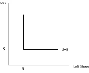
Perfect Complements
Perfect complements are goods that need to be consumed in some fixed ratio. A simple example is left and right shoes, which must be consumed in a 1-for-1 ratio. A left shoe is totally useless without a right shoe, and vice versa.
Consider a bundle containing 2 left shoes and 2 right shoes (bundle A in figure 10). The consumer likes bundle B with 2 left shoes and 4 right shoes equally well since the additional right shoes are useless. Similarly, the consumer likes the bundle with 3 left shoes and 2 right shoes just as well since the additional left shoe is useless. The indifference curve is a right angle. Any bundle on this indifference curve makes the consumer equally happy.
A bundle with 3 left shoes and 3 right shoes would be on a higher indifference curve and would leave the consumer better off than the indifference curve with the bundle containing 2 left shoes and 2 right shoes. As usual, utility increases on the indifference map moving upwards and to the right. See figure 11.
Figure 11: Indifference map for perfect complements
Figure 12: Optimal bundle for perfect complements
Unit 2.3: Consumer Theory (Graphical Presentation): Foundations
of Demand
Michael Malcolm
June 18, 2011
1
Income and Substitution effects (normal goods)
Returning to our example of a consumer buying fish and apples, suppose that the price of a fish rises. According to the ”law of demand”, when the price of fish rises, the quantity of fish demanded falls. There are two conceptually different reasons for this.
• The income effect: As a result of the price increase, the consumer’s real purchasing power falls. This reduction in purchasing power means that the consumer will purchase fewer fish (since fish are a normal good).
• Thesubstitution effect: Because of the higher price of fish, fish are now relatively more expensive and apples are relatively cheaper. As a result, the consumer will substitute and buy apples in place of fish.
It is important to think about these two, conceptually, as separate reasons. The income effect is the reduction resulting from the general decline in purchasing power; the substitution effect is the reduction resulting from substituting cheaper goods.
A similar argument can be made for price decreases. Part of the resulting increase in consumption is a consequence of higher purchasing power, in general. Another part of the increase in consumption is a consequence of substitution towards the good with the lower price.
2
Hicksian Decomposition for a Price Increase (normal good)
To be explicit, let us use a specific numerical example. The consumer’s income is $90 and the price of an apple is $9. Initially, the price of fish is equal to $3. In figure 1, the original budget line isB0. The price of
fish rises to $10, causing the budget line to pivot inwards toB1.
From figure 1, we can see that on the original budget line the consumer’s optimal bundle contains 18 fish, but on the new budget line the consumer’s optimal bundle contains only 6 fish. The higher price of fish caused the consumer to cut his purchases from 18 fish to 6 fish. This reduction is known as thetotal effect. In this case, we say that the total effect is a decrease of 12 fish.
Now, some of this decline in fish purchases will be due to the income effect (the consumer’s purchasing power is lower in general) and some will be due to the substitution effect (the consumer substitutes apples in place of fish since fish are relatively more expensive). Graphically, we want to decompose this total effect into its two elements.
Figure 1: An increase in the price of fish
Figure 3: Optimal bundle on the hypothetical budget line
Observe that the hypothetical budget line BH is a pure income change relative to B1 since the two
are parallel. The price ratios are the same. This shift from B1 to BH is sometimes called the Hicksian compensation. We are leaving the price of fish high (same price ratio) but giving the consumer enough income back to put him on his old indifference curve.
On the hypothetical budget line, the optimal bundle contains 15 fish. See figure 3.
This construction allows us to decompose the total effect into its two parts: the income and substitution effects. Notice that the shift fromBH toB1represents a raw income reduction with no relative price change.
Thus, the reduction from 15 fish to 6 fish, as shown in figure 3, is attributable to the income effect.
On the other hand, the movement fromB0 toBH is a ”twist” that represents a change in relative prices (the slope of the budget line), but gives the consumer enough income to attain the original indifference curve. Thus, the reduction from 18 fish to 15 fish, as shown in figure 3, is attributable to the substitution effect.
Another way to think about it is this – even after we give the consumer back enough money to put him on his old indifference curve (shift from B1 to BH), he still doesn’t buy as many fish as he used to – only
increasing his fish consumption from 6 to 15 fish instead of all the way to 18 fish. This residual 3 fish exactly represents the substitution effect. Even after we’ve given the consumer enough income to compensate him for the price increase, he still buys fewer fish than before since he substitutes apples in place of fish.
We summarize this decomposition in figure 4. Thetotal effect from the price increase,B0 toB1, was to
reduce fish consumption by 12 fish (from 18 fish to 6 fish). Of this 12 fish, theincome effect accounts for 9 units of the decline (from 15 fish to 6 fish) and the substitution effect accounts for 3 units of the decline (from 18 fish to 15 fish).
Of the total reduction in figure 4, the piece from BH to B1 represents a raw income reduction with no
relative price changes – this separates out only the income effect. The piece from B0 to BH represents an increase in the relative price of fish with no reduction in purchasing power – this separates out only the substitution effect. These two combine to form the total effect.
3
Hicksian Decomposition for a Price Decrease (normal good)
Figure 4: Income and substitution effects
as shown in figure 5. Note that the total effect is an increase in consumption of fish from 6 fish to 18 fish, as illustrated on the diagram.
We can follow the same logic as before to separate out the income and the substitution effects. We take the new budget line and shift it until it is parallel to the old indifference curve to form the hypothetical budget line. The construction of this hypothetical budget line is shown in figure 6.
Notice that, in figure 6, the hypothetical budget line involves taking income away from the consumer. The point is, at the new prices, to change income such that the consumer is on his old indifference curve. In this case, when price falls and the consumer is on a higher indifference curve, we need to take income away in order to put him back on the original, lower indifference curve.
Thesubstitution effect is the piece of the increase from 6 fish to 9 fish, which considers the relative price change (pivoting fromB0 toBH) but does not incorporate any change in purchasing power.
The income effect is the piece of the increase from 9 fish to 18 fish representing the increase in raw purchasing power fromBHtoB1. The two budget lines are parallel, so since the relative prices are the same
this only incorporates an income effect, with no substitution effect.
Figure 7 summarizes. Of the total increase in consumption from 6 fish to 18 fish, 3 of the fish are attributable to the substitution effect and the other 9 fish are attributable to the income effect.
4
Inferior and Giffen Goods
Anormal good is one for which demand rises as income rises. Aninferior good is one for which demand falls when income rises. A Giffen good is one for which demand rises as the price of the product rises (a very unusual case).
Figure 5: Total effect from a price reduction
Figure 7: Income and substitution effects for a price reduction
overall purchasing power is lower. Both result in a reduction of fish purchases.
The effect of an increase in the price of fish is an unequivocal reduction in the consumer’s demand for fish. Thus, a normal good cannot be a Giffen good.
However, for an inferior good (rice), the substitution and income effects work in the opposite direction. If the price of rice rises, then as usual the substitution effect spurs the consumer to reduce rice purchases and substitute other goods. The income effect, on the other hand, reflects lower purchasing power. Since rice is an inferior good, lower purchasing power causes the consumer to buymore rice. That is, the substitution effect causes the consumer to buy less rice, while the income effect causes the consumer to buy more rice.
In this case, notice that if the income effect is stronger than the substitution effect, then the net result is that a higher price of rice results in anincreasein the consumer’s demand for rice. This is exactly the Giffen effect – so a Giffen good must be an inferior good where the income effect is stronger than the substitution effect.
It’s important to be clear on the overlap between the two. Not every inferior good is a Giffen good. If the substitution effect is larger than the income effect, then still for an inferior good an increase in price will result in a reduction in demand. However, if for an inferior good the income effect is stronger than the substitution effect, then a price increase will result in an increase in the consumer’s demand, and so the Giffen effect occurs.
While not every inferior good must be a Giffen good, a Giffen good must be an inferior good. A normal good cannot be a Giffen good. For a normal good, both the income and the substitution effects from a price increase result in a reduction in the consumer’s demand, so the Giffen effect is not possible.
A Giffen good violates the law of demand: an increase in the price of a Giffen good causes quantity demanded to rise, and a decrease in price causes quantity demanded to fall.
Figure 8: Change in quantity demanded resulting from price increase
This is the golden recipe for a Giffen good. When the price of potatoes fell, the income effect was large since consumers saw a substantial increase in their purchasing power. They used this additional purchasing power to buy better foods, and thus bought fewer potatoes. However, since potatoes were the only cheap, staple food, there was not much substitution towards potatoes and away from anything else. This combination of a large income effect for an inferior good and very little substitution effect meant that a decline in the price of potatoes resulted in a reduction in consumers’ demand for potatoes – violating the law of demand and creating the Giffen effect.
This example would be hard to replicate in today’s economy since there are many cheap staple foods available to consumers, and no single commodity accounts for an unusually large share of most consumers’ budgets. That is, the income effect is smaller today at the same time that the substitution effect is stronger, all of which work against the Giffen effect.
5
Marshallian Demand Curves
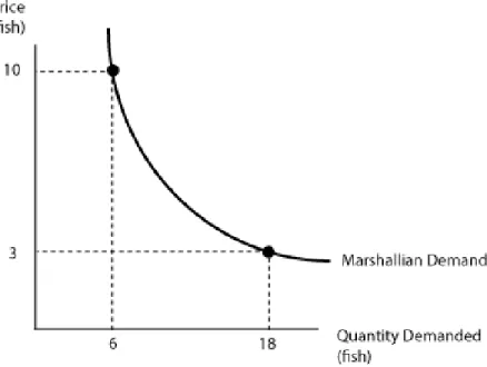
A demand curve relates the quantity of a good that a consumer purchases to its price. Drawing a demand curve is easy: just find the optimal bundle on various budget constraints that reflect different prices of the good.
Returning to the original example, recall that the budget line shifted from B0to B1 when the price of a
fish rose from $3 to $10. See figure 8 to review.
When the price of fish is $3 (budget constraint B0), the consumer’s optimal bundle contains 18 fish.
When the price of fish rises to $10 (budget constraintB1), the consumer’s optimal bundle contains 6 fish.
These are two points on the demand curve – how much fish the consumer wants to buy at various prices. This demand curve is sketched in figure 9.
This demand curve is called a Marshallian demand curve. Observe two things. First, it incorporates both the income effect and the substitution effect since the reduction from 6 fish to 18 fish was the total effect resulting from the price increase. Second, utility falls as price rises and we move leftward along the curve. The optimal bundle onB1in figure 8 is on a lower indifference curve than the optimal bundle onB0.
Figure 9: Marshallian demand curve
6
Hicksian Demand Curves
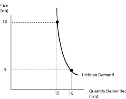
Consider an alternative construction. When the price of fish rises from $3 to $10, rather than looking at the new bundle, look at thecompensated bundle resulting after the price increase. For example, see figure 10.
When price rises from $3 to $10, the consumer’s demand for fish drops from 18 fish to 6 fish. This is reflected in the Marshallian demand curve. However, if we consider the Hicksian compensated bundle, the consumer’s demand drops only from 18 fish to 15 fish when the price rises from $3 to $10. These are two points on theHicksian demand curve, as shown in figure 11.
So the Hicksian demand curve shows what happens after price changes and a compensation that returns consumers to the original indifference curve.
Comparing with the Marshallian demand curve, notice two differences. First, the Hicksian demand curve incorporates only the substitution effect. When price rises, we give the consumer an income transfer sufficient to wash away the income effect, so the reduction (e.g. from 18 fish to 15 fish in figure 10) represents only the part of the reduction in consumer demand due to the substitution effect. Second, the curve is constructed so that utility is constant along a Hicksian demand curve. Both bundles used to construct the Hicksian demand curve are on the same indifference curve.
Figure 10: Compensated change in quantity demanded resulting from price
Unit 3.1: Calculating Demand Functions
Michael Malcolm
June 18, 2011
1
Utility Functions
Utility is a numerical measure of happiness. We will express consumer preferences in terms of a utility function that tells us the consumer’s happiness level as a function of the commodities he consumes.
The important property of utility functions is that the exact number means nothing. The only thing that matters is that higher utility numbers are better than lower utility numbers. In other words, we say that utility is anordinal and not acardinal measure. Any two functions that order bundles in the same way represent the same consumer preferences, regardless of whether the exact utility numbers are the same.
For example, consider a consumer who buys apples Aand bananasB. A possible utility function is
U(A, B) =A2B3
Note that, asA orB increases, utility increases – meaning that the consumer is better off.
Now, the marginal utility of apples is the additional utility that the consumer obtains from one more apple. As such, it is the partial derivative of the utility function with respect toA.
M UA=
∂U
∂A = 2AB
3
Similarly, the marginal utility of an additional banana:
M UB=
∂U ∂B = 3A
2B2
The marginal rate of substitution is the ratio of the marginal utilities.
M RS= M UA M UB
= 2AB
3
3A2B2 =
2 3
B
A
Recall that the MRS represents the number of bananas that the consumer is willing to give up in order to obtain one more apple. Note that the MRS falls asArises, which makes economic sense. As a consumer gets more and more apples, he’s not willing to give up as many bananas to obtain an additional apple.
2
Indifference Curves
Figure 1: Indifference curve forU(A, B) =A2B3
(A, B) = (8,1)⇒U(A, B) = 8213= 64 (A, B) = (1,4)⇒U(A, B) = 1243= 64 (A, B) = (1.54,3)⇒U(A, B) = 1.54233= 64
Since all three bundles (A, B) ={(8,1),(1,4),(1.54,3)} give the consumer the same utility, this means that all these bundles leave the consumer equally well-off. In other words, all are on the same indifference curve. See figure 1 for a sketch of this indifference curve. These are all the bundles that generateU = 64. If we graphed out all the bundles that generateU = 100, this would be a higher indifference curve – all these bundles would leave the consumer better off.
As another example, consider the utility functionU(x1, x2) =
√
x1x2. Notice that the following bundles
all generateU = 2.
(x1, x2) ={(4,1),(1,4),(2,2)}
Similarly, the following bundles all generateU = 4.
(x1, x2) ={(16,1),(1,16),(2,8),(8,2),(4,4)}
Figure 2 diagrams both of these indifference curves.
To reiterate, all bundles on the U = 2 curve leave the consumer equally well off. Similarly, the bundles on theU = 4 curve generate a higher level of utility and therefore leave the consumer better off.
3
Calculating Demands: Example 1
Consider a consumer with income ofY = 100 whose utility function is U(A, B) =A2B3. The price of an apple is PA= 4 and the price of a banana is PB = 2. How should this consumer allocate his income over
Figure 2: Indifference map forU(x1, x2) =
√
This is the fundamental consumer choice problem. The goal is for the consumer to be as well-off as possible, but the bundle selected must be affordable. We call this aconstrained maximization problem. That is, the goal is to maximize utilityU(A, B) =A2B3, but subject to picking a combination ofA andB that
is on the budget constraint.
Writing the budget constraint mathematically is simple. The consumer buys A apples, paying $4 for each apple, so his expenditure on apples is 4A. Similarly, he buysB bananas, paying $2 for each banana, so his expenditure on bananas is 2B. The consumer’s total expenditure on apples and bananas must add up to his total income of $100. Expressing this algebraically:
4A+ 2B= 100
Expressing our problem formally, our goal is to maximizeU(A, B) =A2B3subject to the constraint that 4A+ 2B = 100.
The technique ofLagrange multipliers is designed precisely to solve constrained optimization problems. This technique can be applied to any problem with the following form:
maxf(X) s.t. g(X) = 0
In English, this is read ”maximize f(X) subject to G(X) = 0”. In this case, the utility function f(A, B) =A2B3is the function we are maximizing. The constraint isg(A, B) = 100−4A−2B. Notice that
the budget constraint is set equal to zero in order to apply the Lagrange multiplier technique.
With this constrained optimization problem in hand, formulate the Lagrangian. Here λ is called the
Lagrange multiplier.
L=A2B3+λ(100−4A−2B)
Next, take the partial derivatives of the Lagrangian with respect to the two choice variables (AandBin our example), and also with respect to the lagrange multiplier λ. Set these derivatives equal to zero. This set of equations is known as thefirst order conditions.
∂L
∂A = 2AB
3+ (−4λ) = 0
∂L
∂A = 3A
2B2+ (−2λ) = 0
∂L
∂λ = 100−4A−2B= 0
Next, solve all but the last first order condition forλ.
2AB3= 4λ⇒λ=2AB
3
4
3A2B2= 2λ⇒λ= 3A
2B2
2
2AB3
4 =
3A2B2
2 2AB3
4B2 =
3A2B2 2B2
1 2AB=
3 2A
2
AB= 3A2
B=3A
2
A = 3A
Now, since we know that B= 3A, we can substitute this back into the budget constraint to solve.
4A+ 2B= 100
4A+ 2[3A] = 100
4A+ 6A= 100
10A= 100⇒A= 10
Now, using B= 3A, we find
B= 3A= 3(10) = 30
This consumer maximizes utility by buyingA= 10 apples andB = 30 bananas. With apples at $4 each and bananas at $2 each, it is easy to check that this satisfies the budget constraint.
4
Calculating Demands: Example 2
Above, we solved for consumer demands given specific prices and income. Sometimes, though, we might want to solve for demands atany prices and income. That is, our final demand functions will be equations that depend on income and prices – one can then plug in any prices and income to find consumer demands for that particular set of prices and income.
To illustrate, suppose that a consumer buys 2 goods: x1 and x2. His utility function is U(x1, x2) =
ln(x1) + 2 ln(x2).
For a more general version of the budget line, let the prices of the two goods be P1 andP2, and let the
consumer’s income beY. Since his expenditure onx1 isP1x1 and his expenditure onx2 isP2x2, his budget
constraint is:
P1x1+P2x2=Y
Formulating the problem formally, the consumer solves:
max ln(x1) + 2 ln(x2) s.t. P1x1+P2x2=Y
The Lagrangian is:
The first order conditions are:
∂L
∂x1
= 1 x1
−λP1= 0
∂L
∂x2
= 2 x2
−λP2= 0
∂L
∂λ =Y −P1x1−P2x2= 0
Solving the first two first order conditions forλ:
1 x1
=λP1⇒λ=
1 P1x1
2 x2
=λP2⇒λ=
2 P2x2
Equating the expressions forλ:
1 P1x1
= 2
P2x2
P2x2= 2P1x1
x1=
P2x2
2P1
Substituting this back into the budget constraint:
P1x1+P2x2=Y
P1
P
2x2
2P1
+P2x2=Y
1
2(P2x2) +P2x2=Y 3
2(P2x2) =Y
x2=
2 3
Y
P2
Usingx1=P22Px2
1 , which we derived earlier, we can solve out for
x1=
P2 2 3 Y P2 2P1
x1=
1 3
Y
P1