Derek Atherton
Control Engineering
2nd edition
ISBN 978-87-403-0473-2
Control Engineering: An introduction with the use of Matlab
Contents
Preface 9
About the author 10
1 Introduction 11
1.1 What is Control Engineering? 11
1.2 Contents of the Book 12
1.3 References 14
2 Mathematical Model Representations of Linear Dynamical Systems 15
2.1 Introduction 15
2.2 The Laplace Transform and Transfer Functions 16
2.3 State space representations 19
2.4 Mathematical Models in MATLAB 22
2.5 Interconnecting Models in MATLAB 24
Control Engineering Contents
3 Transfer Functions and Their Responses 27
3.1 Introduction 27
3.2 Step Responses of Some Specific Transfer Functions 29
3.3 Response to a Sinusoid 35
4 Frequency Responses and Their Plotting 38
4.1 Introduction 38
4.2 Bode Diagram 38
4.3 Nyquist Plot 44
4.4 Nichols Plot 47
5 The Basic Feedback Loop 48
5.1 Introduction 48
5.2 The Closed Loop 49
5.3 System Specifications 50
5.4 Stability 54
6 More on Analysis of the Closed Loop System 58
6.1 Introduction 58
6.3 The Root Locus 60
6.4 Relative Stability 63
6.5 M and N Circles 66
7 Classical Controller Design 68
7.1 Introduction 68
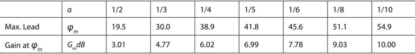
7.2 Phase Lead Design 69
7.3 Phase Lag Design 76
7.4 PID Control 79
7.5 References 89
8 Parameter Optimisation for Fixed Controllers 90
8.1 Introduction 90
8.2 Some Simple Examples 91
8.3 Standard Forms 95
8.4 Control of an Unstable Plant 98
8.5 Further Comments 100
Control Engineering Contents
9 Further Controller Design Considerations 102
9.1 Introduction 102
9.2 Lag-Lead Compensation 102
9.3 Speed Control 105
9.4 Position Control 106
9.5 A Transfer Function with Complex Poles 107
9.6 The Effect of Parameter Variations 111
9.7 References 117
10 State Space Methods 118
10.1 Introduction 118
10.2 Solution of the State Equation 118
10.3 A State Transformation 120
10.4 State Representations of Transfer Functions 121
10.5 State Transformations between Different Forms 126
10.6 Evaluation of the State Transition Matrix 127
10.7 Controllability and Observability 128
11 Some State Space Design Methods 131
11.1 Introduction 131
11.2 State Variable Feedback 131
11.3 Linear Quadratic Regulator Problem 134
11.4 State Variable Feedback for Standard Forms 135
11.5 Transfer Function with Complex Poles 140
12 Appendix A 142
13 Appendix B 148
14 Appendix C 149
Control Engineering Preface
Preface
It is almost four years since the first edition of this book so it seemed appropriate to reread it carefully again and make any suitable changes. Also during the intervening period I have added two further bookboon books one on ‘An Introduction to Nonlinearity in Control Systems’ and another very recently on ‘Control Engineering Problems with Solutions’. This later book contains worked examples and some problems with answers only, which cover the material in this book and ‘An Introduction to Nonlinearity in Control Systems’. It is hoped that the relevant chapters of ‘Control Engineering Problems with Solutions’ will help the reader gain a better understanding and deeper knowledge of the topics covered in this textbook.
Minor changes have been made to this second edition mainly with respect to a few changes in wording, but sadly despite repeated reading a few minor technical errors were found and corrected, for which I apologise. These were Figure 3.6 which had some incorrect markings and was not very clear due to the numbers chosen giving lines almost on top of each other. This has been corrected by choosing a different frequency for illustrating the frequency response calculation procedure. Further, some negative signs were omitted from equation (2.14), the units of H on page 50 were given incorrectly as were the subscripts on the a’s and a matrix in the material in section 10.5.1, page 131, on transforming to the controllable canonical form. Finally the cover page has been changed to contain a picture which is more relevant to the book.
Derek P. Atherton
About the author
Professor Derek. P. Atherton
BEng, PhD, DSc, CEng, FIEE, FIEEE, HonFInstMC, FRSA
Derek Atherton studied at the universities of Sheffield and Manchester, obtaining a PhD in 1962 and DSc in 1975 from the latter. He spent the period from 1962 to 1980 teaching in Canada where he served on several National Research Council committees including the Electrical Engineering Grants Committee.
He took up the post of Professor of Control Engineering at the University of Sussex in 1980 and is currently retired but has an office at the university, gives some lectures, and has the title of Emeritus Professor and Associate Tutor. He has been active with many professional engineering bodies, serving as President of the Institute of Measurement and Control in 1990, President of the IEEE Control Systems Society in 1995, being the only non North American to have held the position, and as a member of the IFAC Council from 1990–96. He served as an Editor of the IEE Proceedings on Control Theory and Applications (CTA) for several years until 2007 and was formerly an editor for the IEE Control Engineering Book Series. He has served EPSRC on research panels and as an assessor for research grants for many years and also served as a member of the Electrical Engineering Panel for the Research Assessment Exercise in 1992.
His major research interests are in non-linear control theory, computer aided control system design, simulation and target tracking. He has written two books, is a co-author of two others and has published more than 350 papers in Journals and Conference Proceedings. Professor Atherton has given invited lectures in many countries and supervised over 30 Doctoral students.
Control Engineering Introduction
1 Introduction
1.1
What is Control Engineering?
As its name implies control engineering involves the design of an engineering product or system where a requirement is to accurately control some quantity, say the temperature in a room or the position or speed of an electric motor. To do this one needs to know the value of the quantity being controlled, so that being able to measure is fundamental to control. In principle one can control a quantity in a so called open loop manner where ‘knowledge’ has been built up on what input will produce the required output, say the voltage required to be input to an electric motor for it to run at a certain speed. This works well if the ‘knowledge’ is accurate but if the motor is driving a pump which has a load highly dependent on the temperature of the fluid being pumped then the ‘knowledge’ will not be accurate unless information is obtained for different fluid temperatures. But this may not be the only practical aspect that affects the load on the motor and therefore the speed at which it will run for a given input, so if accurate speed control is required an alternative approach is necessary.
This alternative approach is the use of feedback whereby the quantity to be controlled, say C, is measured, compared with the desired value, R, and the error between the two,
E = R – C used to adjust C. This gives the classical feedback loop structure of Figure 1.1.
In the case of the control of motor speed, where the required speed, R, known as the reference is either fixed or moved between fixed values, the control is often known as a regulatory control, as the action of the loop allows accurate speed control of the motor for the aforementioned situation in spite of the changes in temperature of the pump fluid which affects the motor load. In other instances the output C may be required to follow a changing R, which for example, might be the required position movement of a robot arm. The system is then often known as a servomechanism and many early textbooks in the control engineering field used the word servomechanism in their title rather than control.
The use of feedback to regulate a system has a long history [1.1, 1.2], one of the earliest concepts, used in Ancient Greece, was the float regulator to control water level, which is still used today in water tanks. The first automatic regulator for an industrial process is believed to have been the flyball governor developed in 1769 by James Watt. It was not, however, until the wartime period beginning in 1939, that control engineering really started to develop with the demand for servomechanisms for munitions fire control and guidance. With the major improvements in technology since that time the applications of control have grown rapidly and can be found in all walks of life. Control engineering has, in fact, been referred to as the ‘unseen technology’ as so often people are unaware of its existence until something goes wrong. Few people are, for instance, aware of its contribution to the development of storage media in digital computers where accurate head positioning is required. This started with the magnetic drum in the 50’s and is required today in disk drives where position accuracy is of the order of 1µm and movement between tracks must be done in a few ms.
Feedback is, of course, not just a feature of industrial control but is found in biological, economic and many other forms of system, so that theories relating to feedback control can be applied to many walks of life.
1.2
Contents of the Book
The book is concerned with theoretical methods for continuous linear feedback control system design, and is primarily restricted to single-input single-output systems. Continuous linear time invariant systems have linear differential equation mathematical models and are always an approximation to a real device or system. All real systems will change with time due to age and environmental changes and may only operate reasonably linearly over a restricted range of operation. There is, however, a rich theory for the analysis of linear systems which can provide excellent approximations for the analysis and design of real world situations when used within the correct context. Further, simulation is now an excellent means to support linear theoretical studies as model errors, such as the affects of neglected nonlinearity, can easily be assessed.
Control Engineering Introduction
Chapter 3 discusses transfer functions, their zeros and poles, and their responses to different inputs. The following chapter discusses in detail the various methods for plotting steady state frequency responses with Bode, Nyquist and Nichols plots being illustrated in MATLAB. Hopefully sufficient detail, which is brief when compared with many textbooks, is given so that the reader clearly understands the information these plots provide and more importantly understands the form of frequency response expected from a specific transfer function.
The material of chapters 2–4 could be covered in other courses as it is basic systems theory, there having been no mention of control, which starts in chapter 5. The basic feedback loop structure shown in Figure 1.1 is commented on further, followed by a discussion of typical performance specifications which might have to be met in both the time and frequency domains. Steady state errors are considered both for input and disturbance signals and the importance and properties of an integrator are discussed from a physical as well as mathematical viewpoint. The chapter concludes with a discussion on stability and a presentation of several results including the Mikhailov criterion, which is rarely mentioned in English language texts. Chapter 6 first introduces the properties of a time delay before continuing with further material relating to the analysis and properties of the closed loop. Briefly mentioned are the root locus and its plotting using MATLAB and various concepts of relative stability. These include gain and phase margins, sensitivity functions, and M and N circles.
The controller design concepts presented in the previous chapter based on open loop frequency response compensation were regularly used in the early days of control engineering by designers who were adept at sketching Bode diagrams, so that the use of modern software has simply brought more efficiency to the design process. Some significant theoretical work on optimising controller parameters to meet specific performance criteria was also done in the early days but here the limitation was the difficulty of using the theory to obtain results of significance. With modern computation tools numerical approaches can be used to solve these problems either by writing MATLAB programs based on linear system theory or writing optimisation programs around digital simulations in programs such as SIMULINK. These are appropriate industrial design methods which appear to receive little attention in textbooks, possibly because they are not suitable for traditional examinations. Chapter 8 covers parameter optimisation based on integral performance criteria because it allows some simple results to be obtained and concepts understood. Further it leads to a design approach based on closed loop transfer function synthesis, known as standard forms, presented at the end of the chapter. Chapter 9 discusses further aspects of classical controller design and highlights the difficulty of trying to design series compensators for, so called uncertain plants, plants whose parameters may vary or not be accurately known. This leads to consideration of some elegant recent results on uncertain plants but which unfortunately appear too conservative for practical use in many instances.
The final two chapters are concerned with the use of state space methods in control system analysis and design. Chapter 10 provides basic coverage of state space concepts covering state equations and their solution, state transformations, state representations of transfer functions, and controllability and observability. Some state space design methods are covered in Chapter 11, including state variable feedback, LQR design and state variable feedback design to achieve the closed loop standard forms of chapter 8.
1.3 References
Bennett, S. A history of Control Engineering, 1800–1930. IEE control engineering series. Peter Peregrinus, 1979.
Control Engineering Mathematical Model Representations of Linear Dynamical Systems
2 Mathematical Model
Representations of Linear
Dynamical Systems
2.1 Introduction
Control systems exist in many fields of engineering so that components of a control system may be electrical, mechanical, hydraulic etc. devices. If a system has to be designed to perform in a specific way then one needs to develop descriptions of how the outputs of the individual components, which make up the system, will react to changes in their inputs. This is known as mathematical modelling and can be done either from the basic laws of physics or from processing the input and output signals, in which case it is known as identification. Examples of physical modelling include deriving differential equations for electrical circuits involving resistance, inductance and capacitance and for combinations of masses, springs and dampers in mechanical systems. It is not the intent here to derive models for various devices which may be used in control systems but to assume that a suitable approximation will be a linear differential equation. In practice an improved model might include nonlinear effects, for example Hooke’s Law for a spring in a mechanical system is only linear over a certain range; or account for time variations of components. Mathematical models of any device will always be approximate, even if nonlinear effects and time variations are also included by using more general nonlinear or time varying differential equations. Thus, it is always important in using mathematical models to have an appreciation of the conditions under which they are valid and to what accuracy.
Starting therefore with the assumption that our model is a linear differential equation then in general it will have the
form:-A(D)y(t) = B(D)u(t) (2.1)
where D denotes the differential operator d/dt. A(D) and B(D) are polynomials in D with Di = di / dti, the ith derivative, u(t) is the model input and y(t) its output. So that one can write
0 1 2
2 1
1
...
)
(
D
D
a
D
a
D
a
D
a
A
nn n n
n
+
+
+
=
−− −
− (2.2)
0 1 2 2 1
1
...
)
(
D
D
b
D
b
D
b
D
b
B
mm m m
m
+
+
+
=
−− −
− (2.3)
Thus, for example, the differential equation
X
GW
GX
\
GW
G\
GW
\
G
(2.4)
with the dependence of y and u on t assumed can be written
u
D
y
D
D
4
3
)
(
2
1
)
(
2+
+
=
+
(2.5)In order to solve an nth order differential equation, that is determine the output y for a given input u, one
must know the initial conditions of y and its first n-1 derivatives. For example if a projectile is falling under gravity, that is constant acceleration, so that D2y= constant, where y is the height, then in order
to find the time taken to fall to a lower height, one must know not only the initial height, normally assumed to be at time zero, but the initial velocity, dy/dt, that is two initial conditions as the equation is second order (n = 2). Control engineers typically study solutions to differential equations using either Laplace transforms or a state space representation.
2.2
The Laplace Transform and Transfer Functions
Control Engineering Mathematical Model Representations of Linear Dynamical Systems
³
f
V
I
W
H
GW
)
VW (2.6)Since the exponential term has no units the units of s are seconds-1, that is using mks notation s has
units of s-1. If denotes the Laplace transform then one may write [f(t)] = F(s) and -1[F(s)] = f(t). The
relationship is unique in that for every f(t), [F(s)], there is a unique F(s), [f(t)]. It is shown in Appendix A that when the n-1 initial conditions, Dn-1y(0) are zero the Laplace transform of Dny(t) is snY(s). Thus
the Laplace transform of the differential equation (2.1) with zero initial conditions can be written
)
(
)
(
)
(
)
(
s
Y
s
B
s
U
s
A
=
(2.7)or simply
U
s
B
Y
s
A
(
)
=
(
)
(2.8)with the assumed notation that signals as functions of time are denoted by lower case letters and as functions of s by the corresponding capital letter.
If equation (2.8) is written
)
(
)
(
)
(
)
(
)
(
G
s
s
A
s
B
s
U
s
Y
=
=
(2.9)then this is known as the transfer function, G(s), between the input and output of the ‘system’, that is whatever is modelled by equation (2.1). B(s), of order m, is referred to as the numerator polynomial and
A(s), of order n, as the denominator polynomial and are from equations (2.2) and (2.3)
0 1 2 2 1 1
...
)
(
s
s
a
s
a
s
a
s
a
A
nn n n
n
+
+
+
=
−− −
− (2.10)
0 1 2 2 1 1
...
)
(
s
s
b
s
b
s
b
s
b
B
mm m m
m
+
+
+
=
−− −
− (2.11)
Since the a and b coefficients of the polynomials are real numbers the roots of the polynomials are either real or complex pairs. The transfer function is zero for those values of s which are the roots of
When the input u(t) to the differential equation of (2.1) is constant the output y(t) becomes constant when all the derivatives of the output are zero. Thus the steady state gain, or since the input is often thought of as a signal the term d.c. gain (although it is more often a voltage than a current!) is used, and is given by
0 0
/
)
0
(
b
a
G
=
(2.12)If the n roots of A(s) are αi, i = 1….n and of B(s) are βj, j = 1….m, then the transfer function may be written in the zero-pole form
∏
∏
= =−
−
=
n i i m j js
s
K
s
G
1 1)
(
)
(
)
(
α
β
(2.13)where in this case
∏
∏
= =−
−
=
n i i m j jK
G
1 1)
0
(
α
β
(2.14)When the transfer function is known in the zero-pole form then the location of its zeros and poles can be shown on an s plane zero-pole plot, where the zeros are marked with a circle and the poles by a cross.
The information on this plot then completely defines the transfer function apart from the gain K. In
most instances engineers prefer to keep any complex roots in quadratic form, thus for example writing
V V V V V
* (2.15)
Control Engineering Mathematical Model Representations of Linear Dynamical Systems
2.3
State space representations
Consider first the differential equation given in equation (2.4) but without the derivative of u term, that is
X
\
GW
G\
GW
\
G
(2.16)
To solve this equation, as mentioned earlier, one must know the initial values of y and dy/dt, or put another way the initial state of the system. Let us choose therefore to represent y and dy/dt by x1 and x2
the components of a state vector xof order two. Thus we have
x
1=
x
2, by choice, and from substitutionin the differential equation
x
2=
−
4
x
2−
3
x
1+
u
. The two equations can be written in the matrix formu
x
x
+
−
−
=
1
0
4
3
1
0
(2.17)and the output y is simply, in this case, the state x1 and can be written
For this choice of state vector the representation is often known as the phase variable representation. The solution for no input, that is u = 0, from an initial state can be plotted in an x1-x2 plane, known as a phase plane with time a parameter on the solution trajectory. Equation (2.17) is a state equation and (2.18) an output equation and together they provide a state space representation of the differential equation or the system described by the differential equation.
Since this system has one input, u, and one output, y, it is often referred to as a input single-output (SISO) system. The choice of the state variable xis not unique and more will be said on this later, but the point is easily illustrated by considering the simple R-C circuit in Figure 2.2. If one derives the differential equation for the output voltage in terms of the input voltage, it will be a second order one similar to equation (2.16) and one could choose as in that equation the output, the capacitor voltage, and its derivative as the components of the state variable, or simply the states, to have a representation similar to equation (2.17). From a physical point of view, however, any initial non zero state will be due to charge stored in one or both of the two capacitors and therefore it might be more appropriate to choose the voltages of these two capacitors as the states.
Figure 2.2 Simple R-C circuit.
In the state space representation of (2.17) and (2.18) x1 is the same as y so that for the state equation (2.18) the transfer function between U(s) and X1(s) is obviously
3
4
1
)
(
)
(
2 1
+
+
=
s
s
s
U
s
X
(2.19)
That is x1 replacing y in the transfer function corresponding to the differential equation (2.16). Now the transfer function corresponding to equation (2.5) is
3
4
1
2
)
(
)
(
2
+
+
+
=
s
s
s
s
U
s
Y
(2.20)
which can be written as
)
(
)
(
2
)
(
)
(
1
1
s
X
s
sX
s
U
s
Y
=
+
Control Engineering Mathematical Model Representations of Linear Dynamical Systems
Since in our state representation
x
1=
x
2, which in transform terms is sX1(s) + X2(s), this means in thiscase with the same state equation the output equation is now y = 2x2+x1. Thus a state space representation for equation (2.5) is
u
x
x
+
−
−
=
1
0
4
3
1
0
,y
=
(
1
2
)
x
(2.22)It is easy to show that for the more general case of the differential equation (2.1) a possible state space representation, which is known as the controllable canonical form, illustrated for m < n-1, is
u
x
a
a
a
a
x
n
+
−
−
−
−
=
−1
.
.
.
.
0
0
0
.
.
.
.
1
.
.
.
.
.
.
.
0
1
0
.
.
.
.
.
.
.
.
.
.
.
.
.
.
.
.
.
.
.
.
.
0
.
.
0
1
0
0
0
0
.
.
.
0
1
0
0
0
.
.
.
.
0
1
0
1 2 1 0
(2.23)(
b
b
b
)
x
y
=
0 1...
m−11
...
0
(2.24)In matrix form the state and output equations can be written
%X $[
[ \ &[ (2.25)
where the state vector, x, is of order n, the A matrix is nxn, B is a column vector of order, n, and C is a row vector of order, n. Because B and C are vectors for the SISO system they are often denoted by b
and cT, respectively. Also in the controllable canonical form representation given above the A matrix
and B vector take on specific forms, the former having the pole polynomial coefficients in the last row and the latter being all zeros apart from the unit value in the last row. If m and n are of the same order, for example if they are both 2 and the corresponding transfer function is
3 4 6 5 2 2 + + + + s s s
s , then this can be
written as 1 2+43+3 + +
s s
s , which means there is a unit gain direct transmission between input and output,
then the state representation takes the more general form
%X $[
[ \ &['X (2.26)
Thus, in conclusion, a mathematical model of a linear SISO dynamical system may be a differential equation, a transfer function or a state space representation. A state space representation has a unique transfer function but the reverse is not the case.
2.4
Mathematical Models in MATLAB
MATLAB, although not the only language with good facilities for control system design, is easy to use and very popular. As well as tools for analysis it also contains a simulation language, SIMULINK, which is also very useful. If it has a weakness it is probably with regard to physical modelling but for the contents of this book, where our starting point is a mathematical model, this is not a problem. Models of system components can be entered into MATLAB either as transfer functions or state space representations. A model is an object defined by a symbol, say G, and its transfer function can be entered in the form
G=tf(num,den) where num and den contain a string of coefficients describing the numerator and
denominator polynomials respectively. MATLAB statements in the text, such as the above for G, will
be entered in bold italics but not in program extracts such as that below. The coefficients are entered beginning with the highest power of s.
Thus the transfer function
3 4
1 2 ) ( 2
+ +
+ =
s s
s s
G , can be entered by
Control Engineering Mathematical Model Representations of Linear Dynamical Systems
>> G=tf(num,den)
Transfer function:
2s + 1 ---s^2 + 4 s + 3
The >> is the MATLAB prompt and the semicolon at the end of a line suppresses a MATLAB response.
This has been omitted from the expression for G so MATLAB responds with the transfer function G as
shown. Alternatively, the entry could have been done in one expression by
typing:->>G=tf([2 1],[1 4 3])
The roots of a polynomial can be found by typing roots before the coefficient string in square brackets. Thus
typing:->> roots(den)
ans =
-3
-1
Alternatively the transfer function can be entered in zero, pole, gain form where the command is in the
form G=zpk(zeros,poles,gain)
Thus for the same example
>> G=zpk([-0.5],[-1;-3],2)
Zero/pole/gain:
2 (s+0.5) ---(s+1) (s+3)
A state space model or object formed from known A,B,C,D matrices, often denoted by (A,B,C,D),can
be entered into MATLAB with the command G=ss(A,B,C,D).
Thus for the same example by entering the following commands one defines the state space model
>> A=[0,1;-3,-4]; >> B=[0;1]; >> C=[1,2]; >> D=0;
>> G=ss(A,B,C,D);
And asking afterwards for the transfer function of the model by typing
>> tf(G) One obtains Transfer function:
2 s + 1 ---s^2 + 4 s + 3
Obviously the above have been very simple examples but hopefully they have covered the basics of putting the mathematical model of a linear dynamical system into MATLAB. The only way to learn is by doing examples and since MATLAB has an excellent help facility the reader should not find this difficult. For a more extensive coverage of MATLAB routines and examples of their use in control engineering the reader is referred to the book given in reference 2.1.
2.5
Interconnecting Models in MATLAB
Control systems are made up of several components, so as well as describing a component by a mathematical model, one needs to deal with the mathematical models for interconnected components. Typically a component is represented as a block with input and output signals and labelled, usually with a transfer function, say G1(s), as shown in Figure 2.3. Strictly speaking if the block is labelled with a transfer function the input and output signals should also be in the s domain, as the block in Figure 2.3 implies
Y(s) = G1(s)U(s) (2.27)
Control Engineering Mathematical Model Representations of Linear Dynamical Systems
Figure 2.3 Block representation of a transfer function
When a second block, with transfer function G2(s), is connected to the output of the first block, to give a series connection, then it is assumed that in making the connection of Figure 2.4 that the second block does not affect the output of the first one. In this case the resultant transfer function of the series combination between input u and output y is G1(s)G2(s), which is obtained directly by substitution from the individual block relationships X(s)=G1(s)U(s) and Y(s)=G2(s)X(s) where x is the output of the first block.
Figure 2.4 Series (or cascade) connection of blocks
If two transfer function models, G1(s) and G2(s) are connected in parallel, as shown in Figure 2.5, then the resultant transfer function between the input u and output y is obtained from the relationships
X1(s) = G1(s)U(s), X2(s) = G2(s)U(s) and Y(s) = X1(s)+X2(s) and is G1(s)+G2(s). It can be obtained in
MATLAB by typing G=G1+G2
Figure 2.5 Parallel connection of blocks
Another connection of blocks which will be used is the feedback connection shown in Figure 2.6. For the negative feedback connection of Figure 2.6 the relationship is Y(s) = G(s)[U(s) – H(s)Y(s)], where the expression in the square brackets is the input to G(s). This can be rearranged to give a transfer function between the input u and output y of
)
(
)
(
1
)
(
)
(
)
(
s
H
s
G
s
G
s
U
s
Y
+
=
. (2.28)If this transfer function is denoted by T(s) then the MATLAB command to obtain T(s) is T=feedback(G,H).
If the positive feedback configuration is required then the statement T=feedback(G,H,sign)can be used where the sign = 1. This can also be used for the negative feedback with sign = -1
Figure 2.6 Feedback connection of blocks.
2.6 Reference
2.1 Xue D., Chen Y. and Atherton D.P. Linear Feedback Control: Analysis and Design in MATLAB,
Control Engineering Transfer Functions and Their Responses
3 Transfer Functions and Their
Responses
3.1
Introduction
As mentioned previously a major reason for wishing to obtain a mathematical model of a device is to be able to evaluate the output in response to a given input. Using the transfer function and Laplace transforms provides a particularly elegant way of doing this. This is because for a block with input U(s) and transfer function G(s) the output Y(s) = G(s)U(s). When the input, u(t), is a unit impulse which is conventionally denoted by δ(t), U(s) = 1 so that the output Y(s) = G(s). Thus in the time domain, y(t) =
g(t), the inverse Laplace transform of G(s), which is called the impulse response or weighting function of the block. The evaluation of y(t) for any input u(t) can be done in the time domain using the convolution integral (see Appendix A, theorem (ix))
GW
W
X
J
W
\
W
W
W
³
(3.1)but it is normally much easier to use the transform relationship Y(s) = G(s)U(s). To do this one needs to find the Laplace transform of the input u(t), form the product G(s)U(s) and then find its inverse Laplace transform. G(s)U(s) will be a ratio of polynomials in s and to find the inverse Laplace transform, the roots of the denominator polynomial must be found to allow the expression to be put into partial fractions with each term involving one denominator root (pole). Assuming, for example, the input is a unit step so that U(s) = 1/s then putting G(s)U(s) into partial fractions will result in an expression for
Y(s) of the form
∑
=
−
+
=
ni i
i
s
C
s
C
s
Y
1 0
)
(
α
(3.2)where in the transfer function G(s) = B(s)/A(s), the n poles of G(s) [zeros of A(s)] are αi, i = 1…n and the coefficients C0 and Ci, i = 1…n, will depend on the numerator polynomial B(s), and are known as the residues at the poles. Taking the inverse Laplace transform yields
∑
=+
=
ni
t i
e
iC
C
t
y
1 0
)
(
αThe first term is a constant C0, sometimes written C0u0(t) because the Laplace transform is defined for t ≥ 0, where u0(t) denotes the unit step at time zero. Each of the other terms is an exponential, which provided the real part of αi is negative will decay to zero as t becomes large. In this case the transfer function is said to be stable as a bounded input has produced a bounded output. Thus a transfer function is stable if all its poles lie in the left hand side (lhs) of the s plane zero-pole plot illustrated in Figure 2.1. The larger the negative value of αi the more rapidly the contribution from the ith term decays to zero. Since any
poles which are complex occur in complex pairs, say of the form α1,α2 = σ ± jω, then the corresponding two residues C1 and C2 will be complex pairs and the two terms will combine to give a term of the form
Control Engineering Transfer Functions and Their Responses
3.2
Step Responses of Some Specific Transfer Functions
In control engineering the major deterministic input signals that one may wish to obtain responses to are a step, an impulse, a ramp and a constant frequency input. The purpose of this section is to discuss step responses of specific transfer functions, hopefully imparting an understanding of what can be expected from a knowledge of the zeros and poles of the transfer function without going into detailed mathematics.
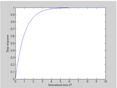
3.1.1 A Single Pole Transfer Function
A transfer function with a single pole is GG(s) = s sKa + = 1
)
( , which may also be written in the so-called time
constant form G*(sV) = .V7
, where K= K1/a and T = 1/a The steady state gain G(0) = K, which is the final
value of the response to a unit step input, and T is called the time constant as it determines the speed of the response. K will have units relating the input quantity to the output quantity, for example °C/V, if the input is a voltage and the output temperature. T will have the same units of time as s-1, normally
seconds. The output, Y(s), for a unit step input is given by
V7
.7
V
.
V7
V
.
V
<
(3.4).Taking the inverse Laplace transform gives the result
)
1
(
)
(
t
K
e
t/Ty
=
−
− (3.5)The larger the value of T (i.e. the smaller the value of a), the slower the exponential response. It can
easily be shown that \7 . 7
GW
G\ DQG\7 . or in words, the output reaches 63.2%
of the final value after a time T, the initial slope of the response is T and the response has essentially
reached the final value after a time 5T. The step response in MATLAB can be obtained by the command
Figure 3.1 Normalised step response for a single time constant transfer function.
3.1.2 Two Complex Poles
Here the transfer function G(s) is often assumed to be of the form
2 2 2 2 ) ( o o o s s s
G ζωω ω
+ +
= . (3..6)
It has a unit steady state gain, i.e G(0) = 1, and poles at
]Z
rZ
]
R
R M
V , which are complex
when ζ < 1. For a unit step input the output Y(s), can be shown after some algebra, which has been done so that the inverse Laplace transforms of the second and third terms are damped cosinusoidal and sinusoidal expressions, to be given by
] Z ]Z ]Z ] Z ]Z ]Z Z Z ] Z
R R R V R RR V R R R
V V V V V V
< (3.7)
Taking the inverse Laplace transform it yields, again after some algebra,
) 1 sin( 1 1 ) ( 2
2 ζ ω ϕ
ζ ζω + − − −
= e− t
t
y o
t o
(3.8)
where
ϕ
=
cos
−1ζ
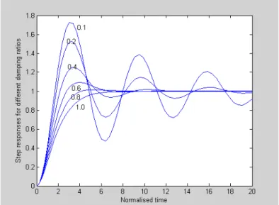
. ζ is known as the damping ratio. It can also be seen that the angle to the negative real axis from the origin to the pole with positive imaginary part is tan−1(1−ζ2)1/2/ζ =cos−1ζ =ϕ.Measurement of the angle φ and this relationship is often used to refer to the damping of complex poles even when not dealing with a second order system. The response on the normalised time scale ωot can be found from Matlab by taking ωo equal to one. The damping of the response then depends on ζ and the
oscillatory behaviour on the normalised damped frequency, that is ω/ω = 1−ζ2
o . Figure 3.2 shows a
Control Engineering Transfer Functions and Their Responses
The response can be shown to have the following
properties:-1) For ζ = 0 the response is undamped and continues to oscillate with frequency ωo (ωo =1 on the normalised plot)
2) The overshoots and undershoots occur at half periods of the damped frequency,
ω
, that is times of nπ/ω, for integers n greater and equal to 1.3) The first overshoot is
'
H
]S ], then the undershoot is Δ2, the next overshoot is Δ3 andso on.
4) The overshoot is often given as a percentage, i.e.100 Δ, and is shown in Figure 3.3 as a function of ζ.
Figure 3.2 Normalised step response of second order system for different ς
Figure 3.3 Graph of % overshoot as a function of the damping ratio.
3.1.3 The Effect of a Zero
Consider the general transfer function G(s) = B(s)/A(s) again, and also G0(s) = 1/A(s), that is G(s) with
B(s) = 1. As outlined above the effect of a non-unity B(s) will be to give different values of the C coefficients in the partial fraction expansion of equation (3.2). Thus one can find the new partial fraction expansion when B(s) is not a constant and invert to find the time response. There is another way, however, which also helps in understanding the response and that is to recognise that s can be regarded as a derivative operator. Thus, for example, suppose the response of G0(s) to a unit step input is y0(t) then the response of G(s) to a unit step input can be written as
W G \ W E G \ W EG\ W E \ W
Control Engineering Transfer Functions and Their Responses
where the b’s are the coefficients of B(s) in equation (2.11).
To illustrate this consider
V V
V7 V
* VRWKDW
V V V V
V V V
<R
then the solution for y0(t) is
y
0(
t
)
=
0
.
5
(
1
−
e
−t+
e
−2t)
, which cannot have an overshoot as theexponentials decrease with increase in time. Using the above result y(t) is given by
GW H H G 7 H
H W
\ W W W W
It is easy to show mathematically that the response will have an overshoot for T > 1. The responses for
T = 0.5, T = 1 and T = 2 are shown in Figure 3.4, obtained using the following MATLAB statements.
>> G0=tf([1],[1 3 2]); >> step(G0)
>> hold
Current plot held
>> G1=tf([0.5 1],[1 3 2]); >> G2=tf([1 1],[1 3 2]); >> G3=tf([2 1],[1 3 2]); >> step(G1)
>> step(G2) >> step(G3)
The unit impulse, δ(t), is the derivative of the unit step and has a Laplace transform of unity. Thus the response to a unit impulse is the derivative of the response to a unit step.
3.1.4 A 3 Pole Transfer Function
In order to appreciate the response from multiple poles consider the step responses of two transfer functions each with three poles, a real pole and a complex pair. The example transfer functions are written in factored form, which of course corresponds to transfer functions in parallel, and
are:-2
.
0
1
.
0
1
2
.
0
5
.
0
)
(
21
=
+
+
+
s
+
s
s
s
G
and
5
5
.
2
1
2
.
0
5
.
0
)
(
22
=
+
+
+
s
+
s
s
s
G
.Both transfer functions when written with a common denominator have two zeros and each term in
Control Engineering Transfer Functions and Their Responses
Figure 3.5 Step responses of 3 pole transfer functions.
3.3
Response to a Sinusoid
The Laplace transform of sin ωt is ω/(s2 + ω2), so that when the partial fraction expansion is used to get Y(s) it will now be of the form
¦
Q
L L
L
V
&
V
V&
&
V
<
Z
D
(3.10)For a stable transfer function, G(s), all the exponential terms in the summation will eventually go to zero and the inverse Laplace transform of the first term will be expressible as M sin(ωt + φ), a sinusoidal signal of magnitude (or amplitude) M and phase lag φ relative to the input sinusoid, where M and φ will be functions of ω. This is known as the steady state frequency response of G(s), often simply shortened to frequency response. To determine its value it is not necessary to go through the partial fraction and Laplace transform process indicated above as it can be shown that it can be obtained from the complex number G(jω), where M is the modulus and φ the argument of G(jω). This is a very basic property of a linear system that for a sine wave input the output, in the steady state, will also be a sine wave of the same frequency with the magnitude and phase shift dependent on the frequency.
The value of a transfer function G(s) for a specific value of s = s1 is G(s1) and from consideration of the zero-pole representation of equation (2.13) it can be seen that it is given by
Q L L
P M M
3$
3%
.
V
0
where P is the point s1 in the s plane and PBj and PAiare the distances from P to the m zeros, βj and n
poles, αi. Also the argument φ is given by
∑
∑
= =−
=
n i i m j js
1 1 1)
(
θ
ψ
ϕ
(3.12)where θj and ψi are the zero and pole angles respectively, that is the angles measured from the direction of the positive real axis to the lines drawn from zero j to the point P and from pole i to the point, P, respectively. Evaluating the frequency response as ω goes from 0 to ∞ means evaluating the above as s1
goes from 0 to ∞ on the imaginary axis of the s-plane. The value of understanding this is that it enables one to appreciate how M and φ of a frequency response will vary as ω is increased.
As a simple example consider again the transfer function of equation (2.15) that is
V V V V V
* (3.13)
Its zero-pole plot, shown in Figure 2.1, is repeated below as Figure 3.6 but with the edition of lines joining the one zero and three poles to the point P = 3j on the imaginary axis. The lengths of the lines and angles are marked from which it can be seen that the frequency response of G at ω = 3, has
3$ 3$ 3$ 3%
0 (3.14)
and
732
.
7
tan
268
.
4
tan
5
.
1
tan
3
tan
1 1 1 13 2 1
1
−
−
−
=
−−
−−
−−
−=
θ
ψ
ψ
ψ
ϕ
giving R R R R RM
(3.15)Control Engineering Transfer Functions and Their Responses
Magnitude and phase of the output for a sinusoidal input have a very physical meaning but mathematically they are a polar representation of the output, which can therefore be written in the rectangular form for a complex number, that is
G(jω) = M(ω)ejϕ(ω) = X(ω) + jY(ω) (3.16)
The relationships between the polar and rectangular representations are
M(ω) = [X2 (ω) + Y2(ω)] 1/2 (3.17)
φ = a tan 2(Y (ω), X(ω)) (3.18)
a tan 2 is the arctangent function used in MATLAB which correctly gives the phase φ between 0 and
360°. Most books write φ = tan–1(Y(ω) / X(ω)) which is simply incorrect without further qualification
4 Frequency Responses and Their
Plotting
4.1 Introduction
The frequency response of a transfer function G(jω) was introduced in the last chapter. As G(jω) is a complex number with a magnitude and argument (phase) if one wishes to show its behaviour over a
frequency range then one has 3 parameters to deal with the frequency, ω, the magnitude, M, and the
phase φ. Engineers use three common ways to plot the information, which are known as Bode diagrams, Nyquist diagrams and Nichols diagrams in honour of the people who introduced them. All portray the
same information and can be readily drawn in MATLAB for a system transfer function object G(s).
One diagram may prove more convenient for a particular application, although engineers often have a preference. In the early days when computing facilities were not available Bode diagrams, for example, had some popularity because of the ease with which they could, in many instances, be rapidly approximated. All the plots will be discussed below, quoting many results without going into mathematical detail, in the hope that the reader will obtain enough knowledge to know whether MATLAB plots obtained are of the general shape expected.
4.2
Bode Diagram
A Bode diagram consists of two separate plots the magnitude, M, as a function of frequency and the
phase φ as a function of frequency. For both plots the frequency is plotted on a logarithmic (log) scale along the x axis. A log scale has the property that the midpoint between two frequencies ω1 and ω2 is the frequency
ω =
ω
1ω
2. A decade of frequency is from a value to ten times that value and an octave from a value to twice that value. The magnitude is plotted either on a log scale or in decibels (dB), wheredB = 20log10 M. The phase is plotted on a linear scale. Bode showed that for a transfer function with no right hand side (rhs) s-plane zeros the phase is related to the slope of the magnitude characteristic by the relationship
GX
X
GX
G$
_
_
FRWK
ORJ
³
f
f
S
Z
M
(4.1)where φ(ω1) is the phase at frequency ω1,
u
=
log
e(
ω
/
ω
1)
andA
(
ω
)
=
log
e|
G
(
j
ω
)
|
.Control Engineering Frequency Responses and Their Plotting
For two transfer functions G1 and G2 in series the resultant transfer function, G, is their product, this means for their frequency response
)
(
)
(
)
(
j
ω
G
1j
ω
G
2j
ω
G
=
(4.2)which in terms of their magnitudes and phases can be written
2 1
M
M
M
=
andϕ
=
ϕ
1+
ϕ
2 (4.3)Thus since a log scale is used on the magnitude of a Bode diagram this means Bode magnitude plots for two transfer functions in series can be added, as also their phases on the phase diagram. Hence a transfer function in zero-pole form can be plotted on the magnitude and phase Bode diagrams simple by adding the individual contributions from each zero and pole. It is thus only necessary to know the Bode plots of single roots and quadratic factors to put together Bode plots for a complicated transfer function if it is known in zero-pole form.
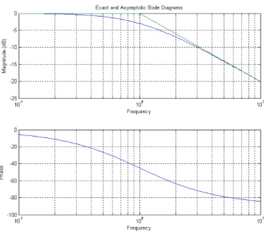
4.2.1 A single time constant
The single pole transfer function is normally considered in time constant form with unit steady state gain, that is
V7 V
*
(4.4)
Figure 4.1 Bode exact and approximate magnitude curves, and phase curve, for a single time constant.
The Bode magnitude plot of a single zero time constant, that is
Control Engineering Frequency Responses and Their Plotting
is simply a reflection in the 0 dB axis of the pole plot. That is the approximate magnitude curve is flat at 0 dB until the break point frequency, 1/T, and then increases at 6 dB/octave. Theoretically as the frequency tends to infinity so does its gain so that it is not physically realisable. The phase curve goes from 0° to +90°.
4.2.2 An Integrator
The transfer function of an integrator, which is a pole at the origin in the zero-pole plot, is 1/s. It is sometimes taken with a gain K, i.e.K/s. Here K will be replaced by 1/T to give the transfer function
V7
V
*
(4.6)On a Bode diagram the magnitude is a constant slope of -6 dB/octave passing through 0 dB at the frequency 1/T. Note that on a log scale for frequency, zero frequency where the integrator has infinite gain (the transfer function can only be produced electronically by an active device) is never reached. The phase is -90° at all frequencies. A differentiator has a transfer function of sT which gives a gain characteristic with a slope of 6 dB/octave passing through 0dB at a frequency of 1/T. Theoretically it produces infinite gain at infinite frequency so again it is not physically realisable. It has a phase of +90° at all frequencies.
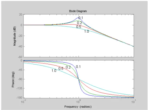
4.2.3 A Quadratic Form
The quadratic factor form is again taken for two complex poles with ζ < 1 as in equation (3.7), that is
2 2
2
2
)
(
o o o
s
s
s
G
ζ
ω
ω
ω
+
+
=
(4.7)Again G(0) = 1 so the response starts at 0 dB and can be approximated by a straight line at 0 dB until ωo
and by a line from ωo at -12 dB/octave. However, this is a very coarse approximation as the behaviour
around ωo is highly dependent on ζ. It can be shown that the magnitude reaches a maximum value
of
2
1 2
1 ζ ζ − =
p
M , which is approximately 1/2ζ for small ζ, at a frequency of ω=ωo 1−2ζ2. This
frequency is thus always less than ωo and only exists for ζ < 0.707. The response with ζ = 0.707 always has magnitude, M < 1. The phase curve goes from 0° to -180° as expected from the original and final slopes of the magnitude curve, it has a phase shift of -90° at the frequency ωo independent of ζ and changes more rapidly near ωo for smaller ζ,as expected due to the more rapid change in the slope of the corresponding magnitude curve. Figure 4.2 shows Bode plots for various values of ζ against normalised frequency ω/ωo. For the quadratic zero
2 2 2 2
) (
o o o s s s
G = + ζωω +ω (4.8)
Figure 4.2 Normalised Bode plots for the quadratic pole form for different ς
4.2.4 An Example Bode Plot
Consider again the one zero, three pole transfer function
V V V
V V
* (4.9)
Dividing numerator and denominator by 2, it can be written in the form
V V V
V V
* (4.10)
For plotting the Bode diagram it can be thought of as 4 transfer
functions:-1) a constant gain of 2
2) a single zero with a breakpoint of 1 3) a single pole with a breakpoint of 2
4) a quadratic pole with natural frequency 1 and damping ratio, ζ = 0.5.
The instruction in MATLAB to obtain the Bode plot of a transfer function object G is simply bode(G).
Control Engineering Frequency Responses and Their Plotting