An Introduction to Combinatorics and Graph Theory - Free Computer, Programming, Mathematics, Technical Books, Lecture Notes and Tutorials

An Introduction to

Combinatorics and Graph

Theory

Creative Commons, 543 Howard Street, 5th Floor, San Francisco, California, 94105, USA. If you distribute this work or a derivative, include the history of the document.

This copy of the text was compiled from source at 14:52 on 1/30/2020.

Contents

1

Fundamentals

7

1.1 Examples . . . 8

1.2 Combinations and permutations . . . 11

1.3 Binomial coefficients . . . 16

1.4 Bell numbers . . . 21

1.5 Choice with repetition . . . 26

1.6 The Pigeonhole Principle . . . 31

1.7 Sperner’s Theorem . . . 35

1.8 Stirling numbers . . . 38

2

Inclusion-Exclusion

43

2.2 Forbidden Position Permutations . . . 46

3

Generating Functions

51

3.1 Newton’s Binomial Theorem . . . 51

3.2 Exponential Generating Functions . . . 54

3.3 Partitions of Integers . . . 57

3.4 Recurrence Relations . . . 60

3.5 Catalan Numbers . . . 64

4

Systems of Distinct Representatives

69

4.2 Partial SDRs . . . 72

4.3 Latin Squares . . . 74

4.4 Introduction to Graph Theory . . . 81

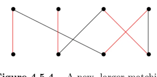
4.5 Matchings . . . 82

5

Graph Theory

89

5.2 Euler Circuits and Walks . . . 94

5.3 Hamilton Cycles and Paths . . . 98

5.4 Bipartite Graphs . . . 101

5.5 Trees . . . 103

5.6 Optimal Spanning Trees . . . 106

5.7 Connectivity . . . 108

5.8 Graph Coloring . . . 116

5.9 The Chromatic Polynomial . . . 122

5.10 Coloring Planar Graphs . . . 123

Contents 5

6

P´

olya–Redfield Counting

133

6.1 Groups of Symmetries . . . 135

6.2 Burnside’s Theorem . . . 138

6.3 P´olya-Redfield Counting . . . 144

A

Hints

149

1

Fundamentals

Combinatorics is often described briefly as being about counting, and indeed counting is a large part of combinatorics. As the name suggests, however, it is broader than this: it is about combining things. Questions that arise include counting problems: “How many ways can these elements be combined?” But there are other questions, such as whether a certain combination is possible, or what combination is the “best” in some sense. We will see all of these, though counting plays a particularly large role.

Graph theory is concerned with various types of networks, or really models of networks called graphs. These are not the graphs of analytic geometry, but what are often described as “points connected by lines”, for example:

... ... ... ... ... ... ... ... ... . . . . . . . . . . . . . . . . . . . . . . . . . . . . . . . . . . . . . . . . . . . . . . . . . . . . . . . . . . . . . . . . . . . . . . . . . . . . . . . . . . . . . . . . ... ... ..._... ... ... ... ... ... ... ... ... ... ... ... ... ... ... ... ... ... ... ... ... ... ..._... ..._... .... • • • • • • •

The preferred terminology is vertex for a point and edge for a line. The lines need not be straight lines, and in fact the actual definition of a graph is not a geometric definition. The figure above is simply a visualization of a graph; the graph is a more abstract object, consisting of seven vertices, which we might name{v1, . . . , v7}, and the collection of pairs of vertices that are connected; for a suitable assignment of names vi to the points in the diagram, the edges could be represented as {v1, v2},{v2, v3},{v3, v4},{v3, v5},{v4, v5},

{v5, v6},{v6, v7}.

1.1 Examples

Suppose we have a chess board, and a collection of tiles, like dominoes, each of which is the size of two squares on the chess board. Can the chess board be covered by the dominoes? First we need to be clear on the rules: the board is covered if the dominoes are laid down so that each covers exactly two squares of the board; no dominoes overlap; and every square is covered. The answer is easy: simply by laying out 32 dominoes in rows, the board can be covered. To make the problem more interesting, we allow the board to be rectangular of any size, and we allow some squares to be removed from the board. What can be say about whether the remaining board can be covered? This is such a board, for example:

.

What can we say? Here is an easy observation: each domino must cover two squares, so the total number of squares must be even; the board above has an even number of squares. Is that enough? It is not too hard to convince yourself that this board cannot be covered; is there some general principle at work? Suppose we redraw the board to emphasize that it really is part of a chess board:

.

1.1 Examples 9 for example:

.

The gray square at the upper right clearly cannot be covered. Unfortunately it is not easy to state a condition that fully characterizes the boards that can be covered; we will see this problem again. Let us note, however, that this problem can also be represented as a graph problem. We introduce a vertex corresponding to each square, and connect two vertices by an edge if their associated squares can be covered by a single domino; here is the previous board:

.. •

.

•

.

•

.

•.. _{• •}

Here the top row of vertices represents the gray squares, the bottom row the white squares. A domino now corresponds to an edge; a covering by dominoes corresponds to a collection of edges that share no endpoints and that areincidentwith (that is, touch) all six vertices. Since no edge is incident with the top left vertex, there is no cover.

Perhaps the most famous problem in graph theory concerns map coloring: Given a map of some countries, how many colors are required to color the map so that countries sharing a border get different colors? It was long conjectured that any map could be colored with four colors, and this was finally proved in 1976. Here is an example of a small map, colored with four colors:

.

that no two connected capitals share a color is clearly the same problem. For the previous map:

.

.

.

•

.

•

.

•

.

•

Any graph produced in this way will have an important property: it can be drawn so that no edges cross each other; this is a planar graph. Non-planar graphs can require more than four colors, for example this graph:

..

• .

•

. •

.

•

.

•

This is called the complete graph on five vertices, denoted K5; in a complete graph, each vertex is connected to each of the others. Here only the “fat” dots represent vertices; intersections of edges at other points are not vertices. A few minutes spent trying should convince you that this graph cannot be drawn so that its edges don’t cross, though the number of edge crossings can be reduced.

Exercises 1.1.

1. Explain why anm×nboard can be covered if eithermorn is even. Explain why it cannot be covered if both mandn are odd.

2. Suppose two diagonally opposite corners of an ordinary 8×8 board are removed. Can the resulting board be covered?

3. Suppose that mandn are both odd. On an m×nboard, colored as usual, all four corners will be the same color, say white. Suppose one white square is removed from any location on the board. Show that the resulting board can be covered.

1.2 Combinations and permutations 11 5. Suppose the square in row 3, column 3 of an 8×8 board is removed. Can the remainder be

covered by 1×3 tiles? Show a tiling or prove that it cannot be done.

6. Remove two diagonally opposite corners of an m×n board, where mis odd and n is even. Show that the remainder can be covered with dominoes.

7. Suppose one white and one black square are removed from an n×n board, n even. Show that the remainder can be covered by dominoes.

8. Suppose ann×nboard,neven, is covered with dominoes. Show that the number of horizontal dominoes with a white square under the left end is equal to the number of horizontal dominoes with a black square under the left end.

9. In the complete graph on five vertices shown above, there are five pairs of edges that cross. Draw this graph so that only one pair of edges cross. Remember that “edges” do not have to be straight lines.

10. Thecomplete bipartite graphK3,3 consists of two groups of three vertices each, with all

possible edges between the groups and no other edges:

... ... ... ... ... ... ... ... ... ... ... ... ... ... ... ... ... ... ... ..._... ..._... ..._... ..._... ..._... ... ... ... ... ... ... ... ... ... ... ... ... ... ... ... ... ..._... ..._... ..._... ..._... ..._... ... ... ... ... ... ... ... ... ... ... ... ... ... ... ... ... ... ... . . . . . . . . . . . . . . . . . . . . . . . . . . . . . . . . . . . . . . . . . . . . . . . . . . . . . . . . . . . . . . . . . . . . . . . . . . . . . . . . . . . . . . . . . . . . . . . . . . . . . . . . . . . . . . . . . . . . . . . . . . . . . . . . . . . . . . . . . . . . . . . . . . . . . . . . . . . . . . . . . . . . . . . . . . . . . . . . . . . . . . . . . . . . . . . . . . . . . . . . . . . . . . . . . . . . . . . . . . . . . . . . . . . . . . . . . . . . . . . . . . . . . . . . . . . . . . . . . . . . . . . . . . . . . . . . . . . . . . . . . . . . . . . . . . . . . . . . . . . . . . . . . . . . . . . . . . . . . . . . . . . . . . . . . . . . . . ... ... ... ... ... ... ... ... ..._... ..._... ..._... ..._... ..._... ... • • • • • •

Draw this graph with only one crossing.

1.2 Combinations and permutations

We turn first to counting. While this sounds simple, perhaps too simple to study, it is not. When we speak of counting, it is shorthand for determining the size of a set, or more often, the sizes of many sets, all with something in common, but different sizes depending on one or more parameters. For example: how many outcomes are possible when a die is rolled? Two dice? ndice? As stated, this is ambiguous: what do we mean by “outcome”? Suppose we roll two dice, say a red die and a green die. Is “red two, green three” a different outcome than “red three, green two”? If yes, we are counting the number of possible “physical” outcomes, namely 36. If no, there are 21. We might even be interested simply in the possible totals, in which case there are 11 outcomes.

Even the quite simple first interpretation relies on some degree of knowledge about counting; we first make two simple facts explicit. In terms of set sizes, suppose we know that setA has size mand set B has sizen. What is the size ofA and B together, that is, the size of A∪B? If we know that A and B have no elements in common, then the size

disjoint, and hence to use it when the circumstances are otherwise. This principle is often called the addition principle.

This principle can be generalized: if setsA1 throughAn are pairwise disjoint and have sizes m1, . . . mn, then the size ofA1∪ · · · ∪An =

∑n

i=1mi. This can be proved by a simple induction argument.

Why do we know, without listing them all, that there are 36 outcomes when two dice are rolled? We can view the outcomes as two separate outcomes, that is, the outcome of rolling die number one and the outcome of rolling die number two. For each of 6 outcomes for the first die the second die may have any of 6 outcomes, so the total is 6 + 6 + 6 + 6 + 6 + 6 = 36, or more compactly, 6·6 = 36. Note that we are really using the addition principle here: set A1 is all pairs (1, x), set A2 is all pairs (2, x), and so on. This is somewhat more subtle than is first apparent. In this simple example, the outcomes of die number two have nothing to do with the outcomes of die number one. Here’s a slightly more complicated example: how many ways are there to roll two dice so that the two dice don’t match? That is, we rule out 1-1, 2-2, and so on. Here for each possible value on die number one, there are five possible values for die number two, but they are a different five values for each value on die number one. Still, because all are the same, the result is 5 + 5 + 5 + 5 + 5 + 5 = 30, or 6·5 = 30. In general, then, if there are mpossibilities for one event, and nfor a second event, the number of possible outcomes for both events together is m·n. This is often called the multiplication principle.

In general, if n events have mi possible outcomes, for i = 1, . . . , n, where each mi is unaffected by the outcomes of other events, then the number of possible outcomes overall is ∏n_i=1mi. This too can be proved by induction.

EXAMPLE 1.2.1 How many outcomes are possible when three dice are rolled, if no two of them may be the same? The first two dice together have 6·5 = 30 possible outcomes, from above. For each of these 30 outcomes, there are four possible outcomes for the third die, so the total number of outcomes is 30·4 = 6·5·4 = 120. (Note that we consider the dice to be distinguishable, that is, a roll of 6, 4, 1 is different than 4, 6, 1, because the first and second dice are different in the two rolls, even though the numbers as a set are the same.)

EXAMPLE 1.2.2 Suppose blocks numbered 1 throughnare in a barrel; we pull out k

of them, placing them in a line as we do. How many outcomes are possible? That is, how many different arrangements of k blocks might we see?

1.2 Combinations and permutations 13 one, the second spot was die number two, the third spot die number three, and 6·5·4 = 6(6−1)(6−2); notice that 6−2 = 6−3 + 1.

This is quite a general sort of problem:

DEFINITION 1.2.3 The number of permutations of n things taken k at a time is

P(n, k) =n(n−1)(n−2)· · ·(n−k+ 1) = n! (n−k)!.

A permutation of some objects is a particular linear ordering of the objects; P(n, k) in effect counts two things simultaneously: the number of ways to choose and order k out of n objects. A useful special case is k =n, in which we are simply counting the number of ways to order alln objects. This is n(n−1)· · ·(n−n+ 1) =n!. Note that the second form ofP(n, k) from the definition gives

n! (n−n)! =

n! 0!.

This is correct only if 0! = 1, so we adopt the standard convention that this is true, that is, we define 0! to be 1.

Suppose we want to count only the number of ways to choosek items out ofn, that is, we don’t care about order. In example1.2.1, we counted the number of rolls of three dice with different numbers showing. The dice were distinguishable, or in a particular order: a first die, a second, and a third. Now we want to count simply how many combinations of numbers there are, with 6, 4, 1 now counting as the same combination as 4, 6, 1.

EXAMPLE 1.2.4 Suppose we were to list all 120 possibilities in example1.2.1. The list would contain many outcomes that we now wish to count as a single outcome; 6, 4, 1 and 4, 6, 1 would be on the list, but should not be counted separately. How many times will a single outcome appear on the list? This is a permutation problem: there are 3! orders in which 1, 4, 6 can appear, and all 6 of these will be on the list. In fact every outcome will appear on the list 6 times, since every outcome can appear in 3! orders. Hence, the list is too big by a factor of 6; the correct count for the new problem is 120/6 = 20.

Following the same reasoning in general, if we have n objects, the number of ways to choose k of them is P(n, k)/k!, as each collection of k objects will be counted k! times by

DEFINITION 1.2.5 The number of subsets of size k of a set of size n (also called an

n-set) is

C(n, k) = P(n, k)

k! =

n!

k!(n−k)! =

(

n k

)

.

The notation C(n, k) is rarely used; instead we use(n_k), pronounced “n choose k”.

EXAMPLE 1.2.6 Considern= 0,1,2,3. It is easy to list the subsets of a smalln-set; a typical n-set is{a1, a2, . . . , an}. A 0-set, namely the empty set, has one subset, the empty set; a 1-set has two subsets, the empty set and {a1}; a 2-subset has four subsets, ∅, {a1},

{a2}, {a1, a2}; and a 3-subset has eight: ∅, {a1}, {a2}, {a3}, {a1, a2}, {a1, a3}, {a2, a3},

{a1, a2, a3}. From these lists it is then easy to compute

(_n

k

)

:

k

0 1 2 3

0 1

n 1 1 1

2 1 2 1

3 1 3 3 1

You probably recognize these numbers: this is the beginning of Pascal’s Triangle. Each entry in Pascal’s triangle is generated by adding two entries from the previous row: the one directly above, and the one above and to the left. This suggests that (n_k) =

(_n−1

k−1

)

+ (n−_k1), and indeed this is true. To make this work out neatly, we adopt the convention that (n_k)= 0 when k <0 or k > n.

THEOREM 1.2.7

(

n k

)

=

(

n−1

k−1

)

+

(

n−1

k

)

.

Proof. A typical n-set is A = {a1, . . . , an}. We consider two types of subsets: those that contain an and those that do not. If a k-subset of A does not contain an, then it is a k-subset of {a1, . . . , an−1}, and there are

(_n−1

k

)

of these. If it does contain an, then it consists of an and k−1 elements of {a1, . . . , an−1}; since there are

(n−1 k−1

)

of these, there are (n_k−₋₁1) subsets of this type. Thus the total number of k-subsets of A is (_kn₋−₁1)+(n−_k1).

Note that when k = 0, (n_k−−₁1) = (n₋−₁1) = 0, and when k = n, (n−_k1) = (n−_n1) = 0, so that (n₀) = (n−₀1) and (n_n) = (n_n−₋1₁). These values are the boundary ones in Pascal’s Triangle.

1.2 Combinations and permutations 15

EXAMPLE 1.2.8 Six people are to sit at a round table; how many seating arrangements are there?

It is not clear exactly what we mean to count here. If there is a “special seat”, for example, it may matter who ends up in that seat. If this doesn’t matter, we only care about the relative position of each person. Then it may or may not matter whether a certain person is on the left or right of another. So this question can be interpreted in (at least) three ways. Let’s answer them all.

First, if the actual chairs occupied by people matter, then this is exactly the same as lining six people up in a row: 6 choices for seat number one, 5 for seat two, and so on, for a total of 6!. If the chairs don’t matter, then 6! counts the same arrangement too many times, once for each person who might be in seat one. So the total in this case is 6!/6 = 5!. Another approach to this: since the actual seats don’t matter, just put one of the six people in a chair. Then we need to arrange the remaining 5 people in a row, which can be done in 5! ways. Finally, suppose all we care about is who is next to whom, ignoring right and left. Then the previous answer counts each arrangement twice, once for the counterclockwise order and once for clockwise. So the total is 5!/2 =P(5,3).

We have twice seen a general principle at work: if we can overcount the desired set in such a way that every item gets counted the same number of times, we can get the desired count just by dividing by the common overcount factor. This will continue to be a useful idea. A variation on this theme is to overcount and thensubtract the amount of overcount.

EXAMPLE 1.2.9 How many ways are there to line up six people so that a particular pair of people are not adjacent?

Denote the people A and B. The total number of orders is 6!, but this counts those orders with A and B next to each other. How many of these are there? Think of these two people as a unit; how many ways are there to line up the AB unit with the other 4 people? We have 5 items, so the answer is 5!. Each of these orders corresponds to two different orders in which A and B are adjacent, depending on whetherA or B is first. So the 6! count is too high by 2·5! and the count we seek is 6!−2·5! = 4·5!.

Exercises 1.2.

1. How many positive factors does 2·34·73·112·475 have? How many doespe1₁ pe2₂ · · ·pen

n have,

where the pi are distinct primes?

3. Six men and six women are to be seated around a table, with men and women alternating. The chairs don’t matter, only who is next to whom, but right and left are different. How many seating arrangements are possible?

4. Eight people are to be seated around a table; the chairs don’t matter, only who is next to whom, but right and left are different. Two people, X and Y, cannot be seated next to each other. How many seating arrangements are possible?

5. In chess, a rook attacks any piece in the same row or column as the rook, provided no other piece is between them. In how many ways can eight indistinguishable rooks be placed on a chess board so that no two attack each other? What about eight indistinguishable rooks on a 10×10 board?

6. Suppose that we want to place 8 non-attacking rooks on a chessboard. In how many ways can we do this if the 16 most ‘northwest’ squares must be empty? How about if only the 4 most ‘northwest’ squares must be empty?

7. A “legal” sequence of parentheses is one in which the parentheses can be properly matched, like ()(()). It’s not hard to see that this is possible precisely when the number of left and right parentheses is the same, and every initial segment of the sequence has at least as many left parentheses as right. For example, ()). . . cannot possibly be extended to a legal sequence. Show that the number of legal sequences of length 2n is Cn =

(_2n n

)

−(2n n+1

)

. The numbers

Cn are called theCatalan numbers.

1.3 Binomial coefficients

Recall the appearance of Pascal’s Triangle in example 1.2.6. If you have encountered the triangle before, you may know it has many interesting properties. We will explore some of these here.

You may know, for example, that the entries in Pascal’s Triangle are the coefficients of the polynomial produced by raising a binomial to an integer power. For example, (x+y)3 = 1·x3+ 3·x2y+ 3·xy2+ 1·y3, and the coefficients 1, 3, 3, 1 form row three of Pascal’s Triangle. For this reason the numbers (n_k)are usually referred to as thebinomial coefficients.

THEOREM 1.3.1 Binomial Theorem

(x+y)n =

(

n

0

)

xn+

(

n

1

)

xn−1y+

(

n

2

)

xn−2y2+· · ·+

(

n n

)

yn = n

∑

i=0

(

n i

)

xn−iyi

Proof. We prove this by induction on n. It is easy to check the first few, say for

n= 0,1,2, which form the base case. Now suppose the theorem is true for n−1, that is,

(x+y)n−1 = n−1

∑

i=0

(

n−1

i

)

xn−1−iyi.

Then

(x+y)n = (x+y)(x+y)n−1 = (x+y) n∑−1

i=0

(

n−1

i

)

1.3 Binomial coefficients 17 Using the distributive property, this becomes

x

n−1

∑

i=0

(

n−1

i

)

xn−1−iyi+y

n∑−1 i=0

(

n−1

i

)

xn−1−iyi

= n∑−1

i=0

(

n−1

i

)

xn−iyi+ n∑−1

i=0

(

n−1

i

)

xn−1−iyi+1.

These two sums have much in common, but it is slightly disguised by an “offset”: the first sum starts with an xny0 term and ends with an x1yn−1 term, while the corresponding terms in the second sum arexn−1y1 and x0yn. Let’s rewrite the second sum so that they match:

n∑−1 i=0

(

n−1

i

)

xn−iyi+ n∑−1

i=0

(

n−1

i

)

xn−1−iyi+1

= n∑−1

i=0

(

n−1

i

)

xn−iyi+ n

∑

i=1

(

n−1

i−1

)

xn−iyi

=

(

n−1 0

)

xn+ n∑−1

i=1

(

n−1

i

)

xn−iyi+ n∑−1

i=1

(

n−1

i−1

)

xn−iyi+

(

n−1

n−1

)

yn

=

(

n−1 0

)

xn+ n∑−1

i=1 (

(

n−1

i

)

+

(

n−1

i−1

)

)xn−iyi+

(

n−1

n−1

)

yn.

Now we can use theorem1.2.7 to get:

(

n−1 0

)

xn+ n−1

∑

i=1 (

(

n−1

i

)

+

(

n−1

i−1

)

)xn−iyi+

(

n−1

n−1

)

yn.

=

(

n−1 0

)

xn+ n∑−1

i=1

(

n i

)

xn−iyi+

(

n−1

n−1

)

yn.

=

(

n

0

)

xn+ n−1

∑ i=1 ( n i )

xn−iyi+

( n n ) yn = n ∑ i=0 ( n i )

xn−iyi.

At the next to last step we used the facts that(n−₀1)=(n₀) and (n_n−₋1₁)=(n_n). Here is an interesting consequence of this theorem: Consider

(x+y)n = (x+y)(x+y)· · ·(x+y).

One way we might think of attempting to multiply this out is this: Go through the n

choices together, getting some term like xxyxyy· · ·yx =xi_yj_{, where of course i+j = n.} If we do this in all possible ways and then collect like terms, we will clearly get

n

∑

i=0

aixn−iyi.

We know that the correct expansion has (n_i)=ai; is that in fact what we will get by this method? Yes: consider xn−iyi. How many times will we get this term using the given method? It will be the number of times we end up with i y-factors. Since there are n

factors (x+y), the number of times we get i y-factors must be the number of ways to pick

i of the (x+y) factors to contribute a y, namely(n_i). This is probably not a useful method in practice, but it is interesting and occasionally useful.

EXAMPLE 1.3.2 Using this method we might get

(x+y)3 =xxx+xxy+xyx+xyy+yxx+yxy+yyx+yyy

which indeed becomes x3+ 3x2y+ 3xy2+y3 upon collecting like terms.

The Binomial Theorem, 1.3.1, can be used to derive many interesting identities. A common way to rewrite it is to substitute y= 1 to get

(x+ 1)n = n

∑

i=0

(

n i

)

xn−i.

If we then substitute x = 1 we get

2n= n

∑

i=0

(

n i

)

,

that is, row nof Pascal’s Triangle sums to 2n. This is also easy to understand combinato-rially: the sum represents the total number of subsets of an n-set, since it adds together the numbers of subsets of every possible size. It is easy to see directly that the number of subsets of an n-set is 2n_{: for each element of the set we make a choice, to include or to} exclude the element. The total number of ways to make these choices is 2·2· · ·2 = 2n_{, by} the multiplication principle.

Suppose now thatn≥1 and we substitute −1 for x; we get

(−1 + 1)n = n

∑

i=0

(

n i

)

(−1)n−i. (1.3.1)

The sum is now an alternating sum: every other term is multiplied by −1. Since the left hand side is 0, we can rewrite this to get

(

n

0

)

+

(

n

2

)

+· · ·=

(

n

1

)

+

(

n

3

)

+· · ·. (1.3.2)

1.3 Binomial coefficients 19 Another obvious feature of Pascal’s Triangle is symmetry: each row reads the same forwards and backwards. That is, we have:

THEOREM 1.3.3 ( n i ) = ( n n−i

)

.

Proof. This is quite easy to see combinatorially: every i-subset of ann-set is associated with an (n− i)-subset. That is, if the n-set is A, and if B ⊆ A has size i, then the complement ofBhas size n−i. This establishes a 1–1 correspondence between sets of size

i and sets of size n−i, so the numbers of each are the same. (Of course, if i= n−i, no proof is required.)

Note that this means that the Binomial Theorem, 1.3.1, can also be written as

(x+y)n = n

∑

i=0

(

n n−i

)

xn−iyi.

or

(x+y)n = n ∑ i=0 ( n i )

xiyn−i.

Another striking feature of Pascal’s Triangle is that the entries across a row are strictly increasing to the middle of the row, and then strictly decreasing. Since we already know that the rows are symmetric, the first part of this implies the second.

THEOREM 1.3.4 For 1≤i≤ ⌊n₂⌋,

( n i ) > ( n i−1

)

.

Proof. This is by induction; the base case is apparent from the first few rows. Write

( n i ) = (

n−1

i−1

)

+

(

n−1

i

) (

n i−1

)

=

(

n−1

i−2

)

+

(

n−1

i−1

)

Provided that 1≤i ≤ ⌊n−₂1⌋, we know by the induction hypothesis that

(

n−1

i

)

>

(

n−1

i−1

)

.

Provided that 1≤i−1≤ ⌊n−₂1⌋, or equivalently 2≤i≤ ⌊n−₂1⌋+ 1, we know that

(

n−1

i−1

)

>

(

n−1

i−2

)

.

Hence if 2≤i≤ ⌊n−₂1⌋, ₍

n i ) > ( n i−1

)

.

Exercises 1.3.

1. Suppose a street grid starts at position (0,0) and extends up and to the right:

(0,0)

A shortest route along streets from (0,0) to (i, j) isi+j blocks long, goingiblocks east and

j blocks north. How many such routes are there? Suppose that the block between (k, l) and (k+ 1, l) is closed, wherek < iandl≤j. How many shortest routes are there from (0,0) to (i, j)?

2. Prove by induction that ∑n_k=0(k_i)=(n+1_i+1)for n≥0 andi≥0.

3. Use a combinatorial argument to prove that ∑n_k=0(k_i)=(n+1_i+1)for n≥0 and i≥0; that is, explain why the left-hand side counts the same thing as the right-hand side.

4. Use a combinatorial argument to prove that (k₂)+(n−₂k)+k(n−k) =(n₂).

5. Use a combinatorial argument to prove that (2n_n)is even.

6. Suppose that Ais a non-empty finite set. Prove that A has as many even-sized subsets as it does odd-sized subsets.

7. Prove that ∑n_k=0(k_i)k=(n+1_i+1)n−(n+1_i+2)forn≥0 and i≥0.

8. Verify that (n+1₂ )+(n₂)=n2. Use exercise2 to find a simple expression for∑n_i=1i2.

9. Make a conjecture about the sums of the upward diagonals in Pascal’s Triangle as indicated. Prove your conjecture is true.

.. 1

1 1

1 2 1

1 3 3 1

1 4 6 4 1

10. Find the number of ways to writenas an ordered sum of ones and twos,n≥0. For example, when n= 4, there are five ways: 1 + 1 + 1 + 1, 2 + 1 + 1, 1 + 2 + 1, 1 + 1 + 2, and 2 + 2.

11. Use (x+ 1)n = ∑n_i=0(n_i)xi to find a simple expression for ∑n_i=0i+11 (n_i)xi+1. Then find a simple expression for ∑n_i=0i+11 (n_i).

12. Use the previous exercise to find a simple expression for∑n_i=0(−1)i 1

i+1 (_n

i )

.

13. Give a combinatorial proof of

k ∑

i=0 (

m i

)(

n k−i

)

=

(

m+n k

)

.

1.4 Bell numbers 21 14. Finish the proof of theorem 1.3.4.

15. Give an alternate proof of theorm 1.3.4by characterizing those i for which(n_i)/(_i−n₁)>1.

16. When is (n_i)/(_i−n₁)a maximum? When is (n_i)/(_i−n₁)= 2?

17. When is (n_i)−(_i−n₁)a maximum?

18. AGalton boardis an upright flat surface with protruding horizontal pins arranged as shown below. At the bottom are a number of bins; if the number of rows is n, the number of bins is n+ 1. A ball is dropped directly above the top pin, and at each pin bounces left or right with equal probability. We assume that the ball next hits the pin below and immediately left or right of the pin it has struck, and this continues down the board, until the ball falls into a bin at the bottom. If we number the bins from 0 to n, how many paths can a ball travel to end up in bin k?

This may be interpreted in terms of probability, which was the intent of Sir Francis Galton when he designed it. Each path is equally likely to be taken by a ball. If many balls are dropped, the number of balls in bin k corresponds to the probability of ending up in that bin. The more paths that end in a bin, the higher the probability. When a very large number of balls are dropped, the balls will form an approximation to the bell curve familiar from probability and statistics. There is an animation of the process

at http://www.math.uah.edu/stat/apps/GaltonBoardExperiment.html. There was once a

very nice physical implementation at the Pacific Science Center in Seattle.

.. _•

.

•

.

•

.

•

.

•

.

•

.

•

.

•

.

•

.

•

.

•

.

•

.

•

.

•

.

•

.

•

.

•

.

•

.

•

.

•

.

•

1.4 Bell numbers

We begin with a definition:

DEFINITION 1.4.1 Apartitionof a setSis a collection of non-empty subsetsAi ⊆S, 1 ≤ i ≤ k (the parts of the partition), such that ∪k_i=1Ai = S and for every i ̸= j,

Ai∩Aj =∅.

EXAMPLE 1.4.2 The partitions of the set {a, b, c} are {{a},{b},{c}}, {{a, b},{c}}, {{a, c},{b}}, {{b, c},{a}}, and {{a, b, c}}.

[n] = {1,2,3, . . . , n}, unless some other set is of interest. We denote the number of parti-tions of an n-element set by Bn; these are theBellnumbers. From the example above, we see that B3 = 5. For convenience we let B0 = 1. It is quite easy to see that B1 = 1 and B2 = 2.

There are no known simple formulas forBn, so we content ourselves with a recurrence relation.

THEOREM 1.4.3 The Bell numbers satisfy

Bn+1 = n ∑ k=0 ( n k )

Bk.

Proof. Consider a partition of S = {1,2, . . . , n+ 1}, A1,. . .,Am. We may suppose that n+ 1 is in A1, and that |A1| = k + 1, for some k, 0 ≤ k ≤ n. Then A2,. . .,Am form a partition of the remainingn−k elements ofS, that is, ofS\A1. There areBn−k partitions of this set, so there are Bn−k partitions of S in which one part is the set A1. There are

(_n

k

)

sets of sizek+ 1 containingn+ 1, so the total number of partitions of S in whichn+ 1 is in a set of size k+ 1 is(n_k)Bn−k. Adding up over all possible values of k, this means

Bn+1 = n ∑ k=0 ( n k )

Bn−k. (1.4.1)

We may rewrite this, using theorem 1.3.3, as

Bn+1 = n

∑

k=0

(

n n−k

)

Bn−k,

and then notice that this is the same as the sum

Bn+1 = n ∑ k=0 ( n k )

Bk,

written backwards.

EXAMPLE 1.4.4 We apply the recurrence to compute the first few Bell numbers:

B1 = 0 ∑ k=0 ( 0 0 )

B0 = 1·1 = 1

B2 = 1 ∑ k=0 ( 1 k )

Bk =

(

1 0

)

B0+

(

1 1

)

B1 = 1·1 + 1·1 = 1 + 1 = 2

B3 = 2 ∑ k=0 ( 2 k )

Bk = 1·1 + 2·1 + 1·2 = 5

B4 = 3 ∑ k=0 ( 3 k )

1.4 Bell numbers 23

The Bell numbers grow exponentially fast; the first few are 1, 1, 2, 5, 15, 52, 203, 877, 4140, 21147, 115975, 678570, 4213597, 27644437.

The Bell numbers turn up in many other problems; here is an interesting example. A common need in some computer programs is to generate a random permutation of 1,2,3, . . . , n, which we may think of as a shuffle of the numbers, visualized as numbered cards in a deck. Here is an attractive method that is easy to program: Start with the numbers in order, then at each step, remove one number at random (this is easy in most programming languages) and put it at the front of the list of numbers. (Viewed as a shuffle of a deck of cards, this corresponds to removing a card and putting it on the top of the deck.) How many times should we do this? There is no magic number, but it certainly should not be small relative to the size of n. Let’s choose n as the number of steps.

We can write such a shuffle as a list of n integers, (m1, m2, . . . , mn). This indicates that at stepi, the number mi is moved to the front.

EXAMPLE 1.4.5 Let’s follow the shuffle (3,2,2,4,1):

(3) : 31245

(2) : 23145

(2) : 23145

(4) : 42315

(1) : 14235

Note that we allow “do nothing” moves, removing the top card and then placing it on top. The number of possible shuffles is then easy to count: there arenchoices for the card to remove, and this is repeatedntimes, so the total number isnn. (If we continue a shuffle for m steps, the number of shuffles is nm.) Since there are only n! different permutations of 1,2, . . . , n, this means that many shuffles give the same final order.

Here’s our question: how many shuffles result in the original order?

EXAMPLE 1.4.6 These shuffles return to the original order: (1,1,1,1,1), (5,4,3,2,1), (4,1,3,2,1).

THEOREM 1.4.7 The number of shuffles of [n] that result in the original sorted order is Bn.

the deck sorted and the partitions. Given a shuffle (m1, m2, . . . , mn), we put into a single set all i such that mi has a single value. For example, using the shuffle (4,1,3,2,1), Since

m2 = m5, one set is {2,5}. All the other values are distinct, so the other sets in the partition are {1}, {3}, and {4}.

Note that every shuffle, no matter what the final order, produces a partition by this method. We are only interested in the shuffles that leave the deck sorted. What we now need is to show that each partition results from exactly one such shuffle.

Suppose we have a partition withk parts. If a shuffle leaves the deck sorted, the last entry, mn, must be 1. If the part containing n is A1, then it must be that mi = 1 if and only if i ∈ A1. If k = 1, then the only part contains all of {1,2, . . . , n}, and the shuffle must be (1,1,1, . . . ,1).

Ifk >1, the last move that is not 1 must be 2, since 2 must end up immediately after 1. Thus, if j2 is the largest index such that j2 ∈/ A1, letA2 be the part containing j2, and it must be that mi = 2 if and only if i ∈ A2. We continue in this way: Once we have discovered which of the mi must have values 1,2, . . . , p, let jp+1 be the largest index such that jp+1 ∈/ A1∪ · · · ∪Ap, let Ap+1 be the part containing jp+1, and then mi = p+ 1 if and only if i ∈ Ap+1. When p = k, all values mi have been determined, and this is the unique shuffle that corresponds to the partition.

EXAMPLE 1.4.8 Consider the partition{{1,5},{2,3,6},{4,7}}. We must havem7 = m4 = 1, m6 =m3 =m2 = 2, and m5 =m1 = 3, so the shuffle is (3,2,2,1,3,2,1).

Returning to the problem of writing a computer program to generate a partition: is this a good method? When we say we want a random permutation, we mean that we want each permutation to occur with equal probability, namely, 1/n!. Since the original order is one of the permutations, we want the number of shuffles that produce it to be exactly nn_{/n!, but n! does not divide n}n_{, so this is impossible. The probability of getting} the original permutation is Bn/nn, and this turns out to be quite a bit larger than 1/n!. Thus, this is not a suitable method for generating random permutations.

The recurrence relation above is a somewhat cumbersome way to compute the Bell numbers. Another way to compute them is with a different recurrence, expressed in the Bell triangle, whose construction is similar to that of Pascal’s triangle:

A1,1

A2,1 A2,2

A3,1 A3,2 A3,3 A4,1 A4,2 A4,3 A4,4

1 1 2

2 3 5

5 7 10 15

1.4 Bell numbers 25

An,k may be interpreted as the number of partitions of {1,2, . . . , n + 1} in which {k+ 1} is the singleton set with the largest entry in the partition. For example, A3,2 = 3; the partitions of 3 + 1 = 4 in which 2 + 1 = 3 is the largest number appearing in a singleton set are {{1},{2,4},{3}}, {{2},{1,4},{3}}, and{{1,2,4},{3}}.

To see that this indeed works as advertised, we need to confirm a few things. First, considerAn,n, the number of partitions of{1,2, . . . , n+ 1}in which{n+ 1}is the singleton set with the largest entry in the partition. Since n+ 1 is the largest element of the set, all partitions containing the singleton {n + 1} satisfy the requirement, and so the Bn partitions of{1,2, . . . , n}together with {n+ 1}are exactly the partitions of interest, that is, An,n =Bn.

Next, we verify that under the desired interpretation, it is indeed true that An,k =

An,k−1 +An−1,k−1 for k > 1. Consider a partition counted by An,k−1. This contains the singleton {k}, and the element k + 1 is not in a singleton. If we interchange k and

k+ 1, we get the singleton {k + 1}, and no larger element is in a singleton. This gives us partitions in which {k + 1} is a singleton and {k} is not. Now consider a partition of {1,2, . . . , n} counted by An−1,k−1. Replace all numbers j > k by j + 1, and add the singleton {k + 1}. This produces a partition in which both {k+ 1} and {k} appear. In fact, we have described how to produce each partition counted byAn,k exactly once, and so An,k =An,k−1+An−1,k−1.

Finally, we need to verify that An,1 = Bn−1. We know that A1,1 = 1 = B0. Now we claim that for n >1,

An,1 = n∑−2 k=0

(

n−2

k

)

Ak+1,1.

In a partition counted by An,1, 2 is the largest element in a singleton, so {n+ 1} is not in the partition. Choose anyk ≥1 elements of{3,4, . . . , n}to form the set containing n+ 1. There are An−k−1,1 partitions of the remaining n−k elements in which 2 is the largest element in a singleton. This accounts for (n−_k2)An−k−1,1 partitions of {1,2, . . . , n+ 1}, or over all k:

n∑−2 k=1

(

n−2

k

)

An−k−1,1 = n∑−2 k=1

(

n−2

n−k−2

)

An−k−1,1 = n∑−3 k=0

(

n−2

k

)

Ak+1,1.

We are missing those partitions in which 1 is in the part containingn+ 1. We may produce all such partitions by starting with a partition counted byAn−1,1 and adding n+ 1 to the part containing 1. Now we have

An,1 =An−1,1+ n−3

∑

k=0

(

n−2

k

)

Ak+1,1 = n−2

∑

k=0

(

n−2

k

)

Ak+1,1.

Exercises 1.4.

1. Show that if{A1, A2, . . . , Ak}is a partition of{1,2, . . . , n}, then there is a unique equivalence

relation ≡ whose equivalence classes are {A1, A2, . . . , Ak}.

2. Supposenis a square-free number, that is, no numberm2dividesn; put another way, square-free numbers are products of distinct prime factors, that is, n = p1p2· · ·pk, where each pi

is prime and no two prime factors are equal. Find the number of factorizations of n. For example, 30 = 2·3·5, and the factorizations of 30 are 30, 6·5, 10·3, 2·15, and 2·3·5. Note we count 30 alone as a factorization, though in some sense a trivial factorization.

3. The rhyme scheme of a stanza of poetry indicates which lines rhyme. This is usually expressed in the form ABAB, meaning the first and third lines of a four line stanza rhyme, as do the second and fourth, or ABCB, meaning only lines two and four rhyme, and so on. A limerick is a five line poem with rhyming scheme AABBA. How many different rhyme schemes are possible for an n line stanza? To avoid duplicate patterns, we only allow a new letter into the pattern when all previous letters have been used to the left of the new one. For example, ACBA is not allowed, since when C is placed in position 2, B has not been used to the left. This is the same rhyme scheme as ABCA, which is allowed.

4. Another way to express the Bell numbers for n >0 is

Bn = n ∑

k=1

S(n, k),

where S(n, k) is the number of partitions of {1,2, . . . , n} into exactly k parts, 1 ≤ k ≤ n. The S(n, k) are the Stirling numbers of the second kind. Find a recurrence relation forS(n, k). Your recurrence should allow a fairly simple triangle construction containing the values S(n, k), and then the Bell numbers may be computed by summing the rows of this triangle. Show the first five rows of the triangle, n∈ {1,2, . . . ,5}.

5. Let An be the number of partitions of {1,2, . . . , n+ 1} in which no consecutive integers

are in the same part of the partition. For example, when n = 3 these partitions are

{{1},{2},{3},{4}}, {{1},{2,4},{3}}, {{1,3},{2},{4}}, {{1,3},{2,4}}, {{1,4},{2},{3}}, so A3 = 5. LetA(n, k) be the number of partitions of {1,2, . . . , n+ 1} into exactly k parts,

in which no consecutive integers are in the same part of the partition. Thus

An = n+1∑

k=2

A(n, k).

Find a recurrence for A(n, k) and then show thatAn =Bn.

1.5 Choice with repetition

1.5 Choice with repetition 27 draw, we get a problem essentially identical to the general dice problem. For example, if there are six balls, numbered 1–6, and we draw three balls with replacement, the number of possible outcomes is 63. Another version of the problem does not replace the ball after each draw, but allows multiple “identical” balls to be in the box. For example, if a box contains 18 balls numbered 1–6, three with each number, then the possible outcomes when three balls are drawn and not returned to the box is again 63. If four balls are drawn, however, the problem becomes different.

Another, perhaps more mathematical, way to phrase such problems is to introduce the idea of a multiset. A multiset is like a set, except that elements may appear more than once. If {a, b} and {b, c} are ordinary sets, we say that the union {a, b} ∪ {b, c} is {a, b, c}, not {a, b, b, c}. If we interpret these as multisets, however, we do write{a, b, b, c}

and consider this to be different than {a, b, c}. To distinguish multisets from sets, and to shorten the expression in most cases, we use a repetition number with each element. For example, we will write {a, b, b, c} as {1·a,2·b,1·c}. By writing {1·a,1·b,1·c} we emphasize that this is a multiset, even though no element appears more than once. We also allow elements to be included an infinite number of times, indicated with ∞ for the repetition number, like {∞ ·a,5·b,3·c}.

Generally speaking, problems in which repetition numbers are infinite are easier than those involving finite repetition numbers. Given a multisetA ={∞·a1,∞·a2, . . . ,∞·an}, how many permutations of the elements of lengthkare there? That is, how many sequences

x1, x2, . . . , xk can be formed? This is easy: the answer is nk.

Now consider combinations of a multiset, that is, submultisets: Given a multiset, how many submultisets of a given size does it have? We say that a multiset A is a submultiset of B if the repetition number of every element of A is less than or equal to its repetition number in B. For example, {20·a,5·b,1·c} is a submultiset of {∞ ·a,5·b,3·c}. A multiset is finite if it contains only a finite number of distinct elements, and the repetition numbers are all finite. Suppose again that A = {∞ ·a1,∞ ·a2, . . . ,∞ ·an}; how many finite submultisets does it have of sizek? This at first seems quite difficult, but put in the proper form it turns out to be a familiar problem. Imagine that we havek+n−1 “blank spaces”, like this:

. . .

Now we place n−1 markers in some of these spots:

∧ ∧ ∧ . . . ∧

This uniquely identifies a submultiset: fill all blanks up to the first ∧ with a1, up to the second witha2, and so on:

So this pattern corresponds to the multiset{1·a2,3·a3, . . . ,1·an}. Filling in the markers ∧ in all possible ways produces all possible submultisets of size k, so there are (k+_n−n−₁1) such submultisets. Note that this is the same as (k+n_k−1); the hard part in practice is remembering that the −1 goes with the n, not thek.

• • •

Summarizing the high points so far: The number of permutations of nthings taken k

at a time without replacement is P(n, k) = n!/(n−k)!; the number of permutations of n

things taken k at a time with replacement is nk. The number of combinations of nthings taken k at a time without replacement is (n_k); the number of combinations of n things taken k at a time with replacement is (k+n_k−1).

• • •

If A ={m1 ·a1, m2·a2, . . . , mn·an}, similar questions can be quite hard. Here is an easier special case: How many permutations of the multisetAare there? That is, how many sequences consist of m1 copies of a1, m1 copies of a2, and so on? This problem succumbs to overcounting: suppose to begin with that we can distinguish among the different copies of each ai; they might be colored differently for example: a red a1, a blue a1, and so on. Then we have an ordinary set with M = ∑n_i=1mi elements and M! permutations. Now if we ignore the colors, so that all copies of ai look the same, we find that we have overcounted the desired permutations. Permutations with, say, the a1 items in the same positions all look the same once we ignore the colors of the a1s. How many of the original permutations have this property? m1! permutations will appear identical once we ignore the colors of the a1 items, since there are m1! permutations of the colored a1s in a given m1 positions. So after throwing out duplicates, the number of remaining permutations is M!/m1! (assuming the other ai are still distinguishable). Then the same argument applies to thea2s: there arem2! copies of each permutation once we ignore the colors of thea2s, so

there are M!

m1!m2!

distinct permutations. Continuing in this way, we see that the number

of distinct permutations once all colors are ignored is

M!

m1!m2!· · ·mn! .

This is frequently written ₍

M

m1 m2 . . . mn

)

,

called a multinomial coefficient. Here the second row has n separate entries, not a single product entry. Note that if n= 2 this is

(

M m1 m2

)

= M!

m1!m2!

= M!

m1! (M −m1)! =

(

M m1

)

. (1.5.1)

1.5 Choice with repetition 29

a2. The number of permutations is the number of ways to choose the m1 locations, which is (_m1M).

EXAMPLE 1.5.1 How many solutions doesx1+x2+x3+x4 = 20 have in non-negative integers? That is, how many 4-tuples (m1, m2, m3, m4) of non-negative integers are solu-tions to the equation? We have actually solved this problem: How many submultisets of size 20 are there of the multiset {∞ ·a1,∞ ·a2,∞ ·a3,∞ ·a4}? A submultiset of size 20 is of the form {m1 ·a1, m2 ·a2, m3 ·a3, m4 ·a4} where

∑

mi = 20, and these are in 1–1 correspondence with the set of 4-tuples (m1, m2, m3, m4) of non-negative integers such that ∑mi = 20. Thus, the number of solutions is

(₂₀₊₄₋₁

20

)

. This reasoning applies in general: the number of solutions to

n

∑

i=1

xi =k

is ₍

k+n−1

k

)

.

This immediately suggests some generalizations: instead of the total number of solu-tions, we might want the number of solutions with the variables xi in certain ranges, that is, we might require that mi ≤xi ≤Mi for some lower and upper boundsmi and Mi.

Finite upper bounds can be difficult to deal with; if we require that 0≤xi ≤Mi, this is the same as counting the submultisets of {M1·a1, M2·a2, . . . , Mn·an}. Lower bounds are easier to deal with.

EXAMPLE 1.5.2 Find the number of solutions to x1+x2+x3+x4 = 20 withx1 ≥0, x2 ≥1, x3 ≥2, x4 ≥ −1.

We can transform this to the initial problem in which all lower bounds are 0. The solutions we seek to count are the solutions of this altered equation:

x1+ (x2−1) + (x3−2) + (x4+ 1) = 18.

If we set y1 = x1, y2 = x2 −1, y3 = x3 −2, and y4 = x4 + 1, then (x1, x2, x3, x4) is a solution to this equation if and only if (y1, y2, y3, y4) is a solution to

y1+y2+y3+y4 = 18,

Exercises 1.5.

1. Suppose a box contains 18 balls numbered 1–6, three balls with each number. When 4 balls are drawn without replacement, how many outcomes are possible? Do this in two ways: assuming that the order in which the balls are drawn matters, and then assuming that order does not matter.

2. How many permutations are there of the letters in Mississippi?

3. How many permutations are there of the multiset{1·a1,1·a2, . . . ,1·an}? 4. Let M =∑n_i=1mi. Ifki<0 for some i, let’s say

(

M k1k2 . . . kn

)

= 0.

Prove that ₍

M m1 m2 . . . mn

) = n ∑ i=1 (

M−1

m1m2 . . . (mi−1) . . . mn )

.

Note that when n= 2 this becomes

(

M m1m2

)

=

(

M−1 (m1−1)m2

)

+

(

M−1

m1 (m2−1) )

.

As noted above in equation 1.5.1, when n= 2 we are really seeing ordinary binomial coeffi-cients, and this can be rewritten as

( M m1 ) = (

M−1

m1−1 )

+

(

M−1

m1 )

,

which of course we already know.

5. The Binomial Theorem (1.3.1) can be written (x+y)n = ∑

i+j=n (

n i j

)

xiyj,

where the sum is over all non-negative integers iandj that sum ton. Prove that form≥2, (x1+x2+· · ·+xm)n =

∑( n

i1i2 . . . im )

xi1 1 x

i2 2 . . . x

im

m .

where the sum is over all i1, . . . , im such thati1+· · ·+im=n. 6. Find the number of integer solutions to

x1+x2+x3+x4+x5= 50, x1≥ −3, x2≥0, x3≥4, x4≥2, x5≥12.

1.6 The Pigeonhole Principle 31

1.6 The Pigeonhole Principle

A key step in many proofs consists of showing that two possibly different values are in fact the same. ThePigeonhole principle can sometimes help with this.

THEOREM 1.6.1 Pigeonhole Principle Suppose thatn+ 1 (or more) objects are put into n boxes. Then some box contains at least two objects.

Proof. Suppose each box contains at most one object. Then the total number of objects is at most 1 + 1 +· · ·+ 1 =n, a contradiction.

This seemingly simple fact can be used in surprising ways. The key typically is to put objects into boxes according to some rule, so that when two objects end up in the same box it is because they have some desired relationship.

EXAMPLE 1.6.2 Among any 13 people, at least two share a birth month.

Label 12 boxes with the names of the months. Put each person in the box labeled with his or her birth month. Some box will contain at least two people, who share a birth month.

EXAMPLE 1.6.3 Suppose 5 pairs of socks are in a drawer. Picking 6 socks guarantees that at least one pair is chosen.

Label the boxes by “the pairs” (e.g., the red pair, the blue pair, the argyle pair,. . .). Put the 6 socks into the boxes according to description.

Some uses of the principle are not nearly so straightforward.

EXAMPLE 1.6.4 Suppose a1, . . . , an are integers. Then some “consecutive sum”ak+

ak+1+ak+2+· · ·+ak+m is divisible by n. Consider these nsums:

s1 =a1

s2 =a1+a2

s3 =a1+a2+a3 ..

.

sn =a1+a2+· · ·+an

end up in the same box, meaning that si modn=sj modn for some j > i; hence sj −si is divisible by n, and sj−si =ai+1+ai+2+· · ·+aj, as desired.

A similar argument provides a proof of theChinese Remainder Theorem.

THEOREM 1.6.5 Chinese Remainder Theorem Ifmandnare relatively prime, and 0 ≤ a < m and 0 ≤ b < n, then there is an integer x such that xmodm = a and

x modn=b.

Proof. Consider the integers a, a+m, a+ 2m, . . . a+ (n−1)m, each with remainder a

when divided by m. We wish to show that one of these integers has remainder b when divided by n, in which case that number satisfies the desired property.

For a contradiction, suppose not. Let the remainders ber0 =a modn,r1 =a+mmod n,. . ., rn−1 =a+ (n−1)mmodn. Label n−1 boxes with the numbers 0,1,2,3, . . . , b− 1, b+ 1, . . . n−1. Put each ri into the box labeled with its value. Two remainders end up in the same box, say ri andrj, with j > i, so ri =rj =r. This means that

a+im=q1n+r and a+jm=q2n+r.

Hence

a+jm−(a+im) =q2n+r−(q1n+r)

(j −i)m= (q2−q1)n.

Since nis relatively prime to m, this means that n|(j−i). But since i and j are distinct and in {0,1,2, . . . , n−1}, 0 < j −i < n, so n ∤ (j −i). This contradiction finishes the proof.

More general versions of the Pigeonhole Principle can be proved by essentially the same method. A natural generalization would be something like this: If X objects are put into n boxes, some box contains at least m objects. For example:

THEOREM 1.6.6 Suppose thatr1, . . . , rnare positive integers. IfX ≥(

∑n

i=1ri)−n+1 objects are put into nboxes labeled 1,2,3, . . . , n, then some box labeled icontains at least

ri objects.

Proof. Suppose not. Then the total number of objects in the boxes is at most (r1−1) + (r2−1) + (r3−1) +· · ·+ (rn−1) = (

∑n

i=1ri)−n < X, a contradiction.

This full generalization is only occasionally needed; often this simpler version is suffi-cient:

COROLLARY 1.6.7 Suppose r > 0 and X ≥ n(r−1) + 1 objects are placed into n