Neural Network Toolbox for MATLAB - Free Computer, Programming, Mathematics, Technical Books, Lecture Notes and Tutorials

Computation

Visualization

Programming

Neural Network Toolbox

For Use with MATLAB

Howard Demuth

Mark Beale

[email protected] Technical support

[email protected] Product enhancement suggestions

[email protected] Bug reports

[email protected] Documentation error reports

[email protected] Order status, license renewals, passcodes

[email protected] Sales, pricing, and general information

508-647-7000 Phone

508-647-7001 Fax

The MathWorks, Inc. Mail 3 Apple Hill Drive

Natick, MA 01760-2098

For contact information about worldwide offices, see the MathWorks Web site.

Neural Network Toolbox User’s Guide

 COPYRIGHT 1992 - 2002 by The MathWorks, Inc.

The software described in this document is furnished under a license agreement. The software may be used or copied only under the terms of the license agreement. No part of this manual may be photocopied or repro-duced in any form without prior written consent from The MathWorks, Inc.

FEDERAL ACQUISITION: This provision applies to all acquisitions of the Program and Documentation by or for the federal government of the United States. By accepting delivery of the Program, the government hereby agrees that this software qualifies as "commercial" computer software within the meaning of FAR Part 12.212, DFARS Part 227.7202-1, DFARS Part 227.7202-3, DFARS Part 252.227-7013, and DFARS Part 252.227-7014. The terms and conditions of The MathWorks, Inc. Software License Agreement shall pertain to the government’s use and disclosure of the Program and Documentation, and shall supersede any conflicting contractual terms or conditions. If this license fails to meet the government’s minimum needs or is inconsistent in any respect with federal procurement law, the government agrees to return the Program and Documentation, unused, to MathWorks.

MATLAB, Simulink, Stateflow, Handle Graphics, and Real-Time Workshop are registered trademarks, and TargetBox is a trademark of The MathWorks, Inc.

Other product or brand names are trademarks or registered trademarks of their respective holders. Printing History: June 1992 First printing

April 1993 Second printing January 1997 Third printing July 1997 Fourth printing

Contents

Preface

Neural Networks . . . xviii

Basic Chapters . . . xx

Mathematical Notation for Equations and Figures . . . xxi

Basic Concepts . . . xxi

Language . . . xxi

Weight Matrices . . . xxi

Layer Notation . . . xxi

Figure and Equation Examples . . . xxii

Mathematics and Code Equivalents . . . xxiii

Neural Network Design Book . . . xxiv

Acknowledgments . . . xxv

1

Introduction

Getting Started . . . 1-2 Basic Chapters . . . 1-2 Help and Installation . . . 1-2

Business Applications . . . 1-5 Aerospace . . . 1-5 Automotive . . . 1-5 Banking . . . 1-5 Credit Card Activity Checking . . . 1-5 Defense . . . 1-6 Electronics . . . 1-6 Entertainment . . . 1-6 Financial . . . 1-6 Industrial . . . 1-6 Insurance . . . 1-6 Manufacturing . . . 1-6 Medical . . . 1-7 Oil and Gas . . . 1-7 Robotics . . . 1-7 Speech . . . 1-7 Securities . . . 1-7 Telecommunications . . . 1-7 Transportation . . . 1-7 Summary . . . 1-7

2

Neuron Model and Network Architectures

Neuron Model . . . 2-2 Simple Neuron . . . 2-2 Transfer Functions . . . 2-3 Neuron with Vector Input . . . 2-5

Data Structures . . . 2-13 Simulation With Concurrent Inputs in a Static Network . . . . 2-13 Simulation With Sequential Inputs in a Dynamic Network . . 2-14 Simulation With Concurrent Inputs in a Dynamic Network . 2-16

Training Styles . . . 2-18 Incremental Training (of Adaptive and Other Networks) . . . . 2-18 Batch Training . . . 2-20

Summary . . . 2-24 Figures and Equations . . . 2-25

3

Perceptrons

Introduction . . . 3-2 Important Perceptron Functions . . . 3-3

Neuron Model . . . 3-4

Perceptron Architecture . . . 3-6

Creating a Perceptron (newp) . . . 3-7 Simulation (sim) . . . 3-8 Initialization (init) . . . 3-9

Learning Rules . . . 3-12

Perceptron Learning Rule (learnp) . . . 3-13

Training (train) . . . 3-16

Clear Network/Data Window . . . 3-30 Importing from the Command Line . . . 3-30 Save a Variable to a File and Load It Later . . . 3-31

Summary . . . 3-33 Figures and Equations . . . 3-33 New Functions . . . 3-36

4

Linear Filters

Introduction . . . 4-2

Neuron Model . . . 4-3

Network Architecture . . . 4-4 Creating a Linear Neuron (newlin) . . . 4-4

Mean Square Error . . . 4-8

Linear System Design (newlind) . . . 4-9

Linear Networks with Delays . . . 4-10 Tapped Delay Line . . . 4-10 Linear Filter . . . 4-10

LMS Algorithm (learnwh) . . . 4-13

Limitations and Cautions . . . 4-18 Overdetermined Systems . . . 4-18 Underdetermined Systems . . . 4-18 Linearly Dependent Vectors . . . 4-18 Too Large a Learning Rate . . . 4-19

Summary . . . 4-20 Figures and Equations . . . 4-21 New Functions . . . 4-25

5

Backpropagation

Overview . . . 5-2

Fundamentals . . . 5-4 Architecture . . . 5-4 Simulation (sim) . . . 5-8 Training . . . 5-8

Faster Training . . . 5-14 Variable Learning Rate (traingda, traingdx) . . . 5-14 Resilient Backpropagation (trainrp) . . . 5-16 Conjugate Gradient Algorithms . . . 5-17 Line Search Routines . . . 5-23 Quasi-Newton Algorithms . . . 5-26 Levenberg-Marquardt (trainlm) . . . 5-28 Reduced Memory Levenberg-Marquardt (trainlm) . . . 5-30

Speed and Memory Comparison . . . 5-32 Summary . . . 5-49

Sample Training Session . . . 5-66

Limitations and Cautions . . . 5-71

Summary . . . 5-73

6

Control Systems

Introduction . . . 6-2

NN Predictive Control . . . 6-4 System Identification . . . 6-4 Predictive Control . . . 6-5 Using the NN Predictive Controller Block . . . 6-6

NARMA-L2 (Feedback Linearization) Control . . . 6-14 Identification of the NARMA-L2 Model . . . 6-14 NARMA-L2 Controller . . . 6-16 Using the NARMA-L2 Controller Block . . . 6-18

Model Reference Control . . . 6-23 Using the Model Reference Controller Block . . . 6-25

Importing and Exporting . . . 6-31 Importing and Exporting Networks . . . 6-31 Importing and Exporting Training Data . . . 6-35

7

Radial Basis Networks

Introduction . . . 7-2 Important Radial Basis Functions . . . 7-2

Radial Basis Functions . . . 7-3 Neuron Model . . . 7-3 Network Architecture . . . 7-4 Exact Design (newrbe) . . . 7-5 More Efficient Design (newrb) . . . 7-7 Demonstrations . . . 7-8

Generalized Regression Networks . . . 7-9 Network Architecture . . . 7-9 Design (newgrnn) . . . 7-10

Probabilistic Neural Networks . . . 7-12 Network Architecture . . . 7-12 Design (newpnn) . . . 7-13

Summary . . . 7-15 Figures . . . 7-16 New Functions . . . 7-18

8

Self-Organizing and

Learn. Vector Quant. Nets

Introduction . . . 8-2 Important Self-Organizing and LVQ Functions . . . 8-2

Distance Funct. (dist, linkdist, mandist, boxdist) . . . 8-14 Architecture . . . 8-17 Creating a Self Organizing MAP Neural Network (newsom) . 8-18 Training (learnsom) . . . 8-19 Examples . . . 8-23

Learning Vector Quantization Networks . . . 8-31 Architecture . . . 8-31 Creating an LVQ Network (newlvq) . . . 8-32 LVQ1 Learning Rule(learnlv1) . . . 8-35 Training . . . 8-36 Supplemental LVQ2.1 Learning Rule (learnlv2) . . . 8-38

Summary and Conclusions . . . 8-40 Self-Organizing Maps . . . 8-40 Learning Vector Quantizaton Networks . . . 8-40 Figures . . . 8-41 New Functions . . . 8-42

9

Recurrent Networks

Introduction . . . 9-2 Important Recurrent Network Functions . . . 9-2

Hopfield Network . . . 9-8 Fundamentals . . . 9-8 Architecture . . . 9-8 Design (newhop) . . . 9-10

Summary . . . 9-15 Figures . . . 9-16 New Functions . . . 9-17

10

Adaptive Filters and

Adaptive Training

Introduction . . . 10-2 Important Adaptive Functions . . . 10-2

Linear Neuron Model . . . 10-3

Adaptive Linear Network Architecture . . . 10-4 Single ADALINE (newlin) . . . 10-4

Mean Square Error . . . 10-7

LMS Algorithm (learnwh) . . . 10-8

Adaptive Filtering (adapt) . . . 10-9 Tapped Delay Line . . . 10-9 Adaptive Filter . . . 10-9 Adaptive Filter Example . . . 10-10 Prediction Example . . . 10-13 Noise Cancellation Example . . . 10-14 Multiple Neuron Adaptive Filters . . . 10-16

Application Scripts . . . 11-2

Applin1: Linear Design . . . 11-3 Problem Definition . . . 11-3 Network Design . . . 11-4 Network Testing . . . 11-4 Thoughts and Conclusions . . . 11-6

Applin2: Adaptive Prediction . . . 11-7 Problem Definition . . . 11-7 Network Initialization . . . 11-8 Network Training . . . 11-8 Network Testing . . . 11-8 Thoughts and Conclusions . . . 11-10

Appelm1: Amplitude Detection . . . 11-11 Problem Definition . . . 11-11 Network Initialization . . . 11-11 Network Training . . . 11-12 Network Testing . . . 11-13 Network Generalization . . . 11-13 Improving Performance . . . 11-15

12

Advanced Topics

Custom Networks . . . 12-2 Custom Network . . . 12-3 Network Definition . . . 12-4 Network Behavior . . . 12-12

Additional Toolbox Functions . . . 12-16 Initialization Functions . . . 12-16 Transfer Functions . . . 12-16 Learning Functions . . . 12-17

Custom Functions . . . 12-18 Simulation Functions . . . 12-18 Initialization Functions . . . 12-24 Learning Functions . . . 12-27 Self-Organizing Map Functions . . . 12-36

13

Network Object Reference

Network Properties . . . 13-2 Architecture . . . 13-2 Subobject Structures . . . 13-6 Functions . . . 13-9 Parameters . . . 13-12 Weight and Bias Values . . . 13-14 Other . . . 13-16

Functions by Network Type . . . 14-2 Functions by Class . . . 14-2 Transfer Functions . . . 14-13 Transfer Function Graphs . . . 14-14

Functions — Alphabetical List . . . 14-19 Reference Headings . . . 14-19

A

Glossary

B

Bibliography

C

Demonstrations and

Applications

D

Simulink

Block Set . . . D-2 Transfer Function Blocks . . . D-2 Net Input Blocks . . . D-3 Weight Blocks . . . D-3 Control Systems Blocks . . . D-4

Block Generation . . . D-5 Example . . . D-5 Exercises . . . D-7

E

Code Notes

Dimensions . . . E-2

Variables . . . E-3 Utility Function Variables . . . E-4

Functions . . . E-7

Code Efficiency . . . E-8

Argument Checking . . . E-9

Preface

Neural Networks . . . . xviii

Basic Chapters . . . . xx

Mathematical Notation for Equations and Figures . . xxi

Basic Concepts . . . xxi

Language . . . xxi

Weight Matrices . . . xxi

Layer Notation . . . xxi

Figure and Equation Examples . . . . xxii

Mathematics and Code Equivalents . . . . xxiii

Neural Network Design Book . . . . xxiv

Neural Networks

Neural networks are composed of simple elements operating in parallel. These elements are inspired by biological nervous systems. As in nature, the network function is determined largely by the connections between elements. We can train a neural network to perform a particular function by adjusting the values of the connections (weights) between elements.

Commonly neural networks are adjusted, or trained, so that a particular input leads to a specific target output. Such a situation is shown below. There, the network is adjusted, based on a comparison of the output and the target, until the network output matches the target. Typically many such input/target pairs are used, in this supervised learning, to train a network.

Batch training of a network proceeds by making weight and bias changes based on an entire set (batch) of input vectors. Incremental training changes the weights and biases of a network as needed after presentation of each individual input vector. Incremental training is sometimes referred to as “on line” or “adaptive” training.

Neural networks have been trained to perform complex functions in various fields of application including pattern recognition, identification, classification, speech, vision and control systems. A list of applications is given in Chapter 1.

Today neural networks can be trained to solve problems that are difficult for conventional computers or human beings. Throughout the toolbox emphasis is placed on neural network paradigms that build up to or are themselves used in engineering, financial and other practical applications.

Neural Network including connections (called weights) between neurons

Input Output

Target

Adjust weights

Neural Networks

The supervised training methods are commonly used, but other networks can be obtained from unsupervised training techniques or from direct design

methods. Unsupervised networks can be used, for instance, to identify groups of data. Certain kinds of linear networks and Hopfield networks are designed directly. In summary, there are a variety of kinds of design and learning techniques that enrich the choices that a user can make.

The field of neural networks has a history of some five decades but has found solid application only in the past fifteen years, and the field is still developing rapidly. Thus, it is distinctly different from the fields of control systems or optimization where the terminology, basic mathematics, and design

procedures have been firmly established and applied for many years. We do not view the Neural Network Toolbox as simply a summary of established

Basic Chapters

The Neural Network Toolbox is written so that if you read Chapter 2, Chapter 3 and Chapter 4 you can proceed to a later chapter, read it and use its functions without difficulty. To make this possible, Chapter 2 presents the fundamentals of the neuron model, the architectures of neural networks. It also will discuss notation used in the architectures. All of this is basic material. It is to your advantage to understand this Chapter 2 material thoroughly.

Mathematical Notation for Equations and Figures

Mathematical Notation for Equations and Figures

Basic Concepts

Scalars-small italic letters.....a,b,c

Vectors - small bold non-italic letters...a,b,c

Matrices - capital BOLD non-italic letters...A,B,C

Language

Vector means a column of numbers.

Weight Matrices

Scalar Element

- row, - column, - time or iteration

Matrix

Column Vector

Row Vector

...

Bias Vector

Scalar Element

Vector

Layer Notation

A single superscript is used to identify elements of layer. For instance, the net input of layer 3 would be shown as n3_.

Superscripts are used to identify the source (l) connection and the

destination (k) connection of layer weight matrices ans input weight matrices. For instance, the layer weight matrix from layer 2 to layer 4 would be shown as LW4,2_.

w_{i j,} ( )t

i j t

W( )t

w_j( )t

w i ( )t

b_i( )t

b( )t

Input Weight Matrix

Layer Weight Matrix

Figure and Equation Examples

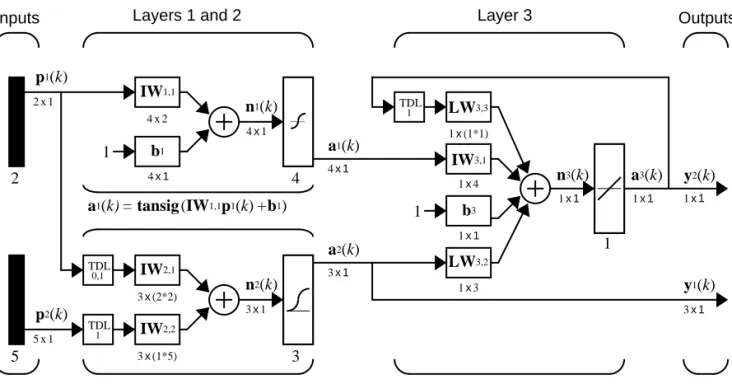
The following figure, taken from Chapter 12 illustrates notation used in such advanced figures.

IW

LWk l,

p1_(k)

a1(k)

1

n1_(k)

2x1

4x2

4x1

4x1

4x1 Inputs

AA

AA

AA

2 4

Layers 1 and 2 Layer 3

a1(k)= tansig(IW1,1p1(k)+b1)

AA

AA

AA

5

3x(2*2)

AA

AA

3x(1*5)

AA

AA

n2_(k)

3x1

3

AA

AA

AA

AA

A

A

p2_(k)

5x1

A

A

1x4

AA

AA

1x3

AA

AA

AA

AA

1

1x1

AA

AA

AA

AA

3x1

a2_(k)

a3(k)

n3(k)

1x1 1x1

1

AA

AA

AA

AA

a2(k)= logsig(IW2,1[p1(k);p1(k-1)]+IW2,2p2(k-1)) 0,1

1

1

a3(k)=purelin(LW3,3a3(k-1)+IW3,1 a1 (k)+b3+LW3,2a2(k))

LW3,2

LW3,3

y2(k)

1x1

y1(k)

Mathematics and Code Equivalents

Mathematics and Code Equivalents

The transition from mathematics to code or vice versa can be made with the aid of a few rules. They are listed here for future reference.

To change from mathematics notation to MATLAB notation, the user needs to:

•Change superscripts to cell array indices. For example,

•Change subscripts to parentheses indices. For example, , and

•Change parentheses indices to a second cell array index. For example,

•Change mathematics operators to MATLAB operators and toolbox functions. For example,

The following equations illustrate the notation used in figures.

p1→p{ }1

p₂→p( )2 p₂1→p{ }1 ( )2

p1(k–1)→p{1,k–1}

ab→a*b

n = w_{1 1,} p₁+w_{1 2,} p₂+...+w_1,Rp_R+b

W

w_{1 1,} w_{1 2,} … w_1,R

w_{2 1,} w_{2 2,} … w_2,R

w_S,1 w_S,2 … w_{S R,}

Neural Network Design Book

Professor Martin Hagan of Oklahoma State University, and Neural Network Toolbox authors Howard Demuth and Mark Beale have written a textbook,

Neural Network Design, published by the Brooks/Cole Publishing Company in 1996 (ISBN 0-534-94332-2). The book presents the theory of neural networks, discusses their design and application, and makes considerable use of MATLAB

and the Neural Network Toolbox. Demonstration programs from the book are used in various chapters of this Guide. (You can find all the book

demonstration programs in the Neural Network Toolbox by typing nnd.)

The book has:

•An INSTRUCTOR’S MANUAL (ISBN 0-534-95049-3) for adopters and •TRANSPARENCY OVERHEADS for class use. The overheads come one to a

page for instructor use and three to a page for student use.

To place an order for the book, call 1-800-354-9706.

To obtain a copy of the INSTRUCTOR’S MANUAL, contact the Brooks/Cole Editorial Office, phone 1-800-354-0092. Ask specifically for an instructor’s manual if you are instructing a class and want one.

You can go directly to the Brooks/Cole Neural Network Design page at

http://brookscole.com/engineering/nnd.html

Once there, you can download the TRANSPARENCY MASTERS with a click on “Transparency Masters(3.6MB).”

Alternatively, you might try the Brooks/Cole Thomson Leaning Web site home page:

http://brookscole.com

Acknowledgments

Acknowledgments

The authors would like to thank:

Martin Hagan of Oklahoma State University for providing the original Levenberg-Marquardt algorithm in the Neural Network Toolbox version 2.0 and various algorithms found in version 3.0, including the new reduced memory use version of the Levenberg-Marquardt algorithm, the coujugate gradient algorithm, RPROP, and generalized regression method. Martin also wrote Chapter 5 and Chapter 6 of this toolbox. Chapter 5 describes new algorithms, suggests algorithms for pre- and post-processing of data, and presents a comparison of the efficacy of various algorithms. Chapter 6 on control system applications, describes practical applications including neural network model predictive control, model reference adaptive control, and a feedback linearization controller.

Joe Hicklin of The MathWorks for getting Howard into neural network research years ago at the University of Idaho, for encouraging Howard to write the toolbox, for providing crucial help in getting the first toolbox version 1.0 out the door, and for continuing to be a good friend.

Jim Tung of The MathWorks for his long-term support for this project. Liz Callanan of The MathWorks for getting us off the such a good start with the Neural Network Toolbox version 1.0.

Roy Lurie of The MathWorks for his vigilant reviews of the developing material in this version of the toolbox.

Matthew Simoneau of The MathWorks for his help with demos, test suite routines, for getting user feedback, and for helping with other toolbox matters.

Sean McCarthy for his many questions from users about the toolbox operation Jane Carmody of The MathWorks for editing help and for always being at her phone to help with documentation problems.

Donna Sullivan and Peg Theriault of The MathWorks for their editing and other help with the Mac document.

Orlando De Jesús of Oklahoma State University for his excellent work in programming the neural network controllers described in Chapter 6.

Bernice Hewitt for her wise New Zealand counsel, encouragement, and tea, and for the company of her cats Tiny and Mr. Britches.

Joan Pilgram for her business help, general support, and good cheer. Teri Beale for running the show and having Valerie and Asia Danielle while Mark worked on this toolbox.

1

Introduction

Getting Started . . . 1-2 Basic Chapters . . . 1-2 Help and Installation . . . 1-2

What’s New in Version 4.0 . . . 1-3 Control System Applications . . . 1-3 Graphical User Interface . . . 1-3 New Training Functions . . . 1-3 Design of General Linear Networks . . . 1-4 Improved Early Stopping . . . 1-4 Generalization and Speed Benchmarks . . . 1-4 Demonstration of a Sample Training Session . . . 1-4

Getting Started

Basic Chapters

Chapter 2 contains basic material about network architectures and notation specific to this toolbox.Chapter 3 includes the first reference to basic functions such as init and adapt. Chapter 4 describes the use of the functions designd and train, and discusses delays. Chapter 2, Chapter 3, and Chapter 4 should be read before going to later chapters

Help and Installation

The Neural Network Toolbox is contained in a directory called nnet. Type help nnet for a listing of help topics.

A number of demonstrations are included in the toolbox. Each example states a problem, shows the network used to solve the problem, and presents the final results. Lists of the neural network demonstration and application scripts that are discussed in this guide can be found by typing help nndemos

Instructions for installing the Neural Network Toolbox are found in one of two

MATLAB documents: the Installation Guide for PC orthe Installation Guide for

What’s New in Version 4.0

What’s New in Version 4.0

A few of the new features and improvements introduced with this version of the Neural Network Toolbox are discussed below.

Control System Applications

A new Chapter 6 presents three practical control systems applications:

•Network model predictive control •Model reference adaptive control •Feedback linearization controller

Graphical User Interface

A graphical user interface has been added to the toolbox. This interface allows you to:

•Create networks

•Enter data into the GUI

•Initialize, train, and simulate networks

•Export the training results from the GUI to the command line workspace •Import data from the command line workspace to the GUI

To open the Network/Data Manager window type nntool.

New Training Functions

The toolbox now has four training algorithms that apply weight and bias learning rules. One algorithm applies the learning rules in batch mode. Three algorithms apply learning rules in three different incremental modes:

•trainb - Batch training function

•trainc - Cyclical order incremental training function •trainr - Random order incremental training function •trains - Sequential order incremental training function

Note We no longer recommend using trainwb and trainwb1, which have been replaced by trainb and trainr. The function trainr differs from trainwb1 in that trainwb1 only presented a single vector each epoch instead of going through all vectors, as is done by trainr.

These new training functions are relatively fast because they generate M-code. The functions trainb, trainc, trainr, and trains all generate a temporary M-file consisting of specialized code for training the current network in question.

Design of General Linear Networks

The function newlind now allows the design of linear networks with multiple inputs, outputs, and input delays.

Improved Early Stopping

Early stopping can now be used in combination with Bayesian regularization. In some cases this can improve the generalization capability of the trained network.

Generalization and Speed Benchmarks

Generalization benchmarks comparing the performance of Bayesian regularization and early stopping are provided. We also include speed benchmarks, which compare the speed of convergence of the various training algorithms on a variety of problems in pattern recognition and function approximation. These benchmarks can aid users in selecting the appropriate algorithm for their problem.

Demonstration of a Sample Training Session

Neural Network Applications

Neural Network Applications

Applications in this Toolbox

Chapter 6 describes three practical neural network control system applications, including neural network model predictive control, model reference adaptive control, and a feedback linearization controller.

Other neural network applications are described in Chapter 11.

Business Applications

The 1988 DARPA Neural Network Study [DARP88] lists various neural network applications, beginning in about 1984 with the adaptive channel equalizer. This device, which is an outstanding commercial success, is a single- neuron network used in long-distance telephone systems to stabilize voice signals. The DARPA report goes on to list other commercial applications, including a small word recognizer, a process monitor, a sonar classifier, and a risk analysis system.

Neural networks have been applied in many other fields since the DARPA

report was written. A list of some applications mentioned in the literature follows.

Aerospace

•High performance aircraft autopilot, flight path simulation, aircraft control systems, autopilot enhancements, aircraft component simulation, aircraft component fault detection

Automotive

•Automobile automatic guidance system, warranty activity analysis

Banking

•Check and other document reading, credit application evaluation

Credit Card Activity Checking

Defense

•Weapon steering, target tracking, object discrimination, facial recognition, new kinds of sensors, sonar, radar and image signal processing including data compression, feature extraction and noise suppression, signal/image identification

Electronics

•Code sequence prediction, integrated circuit chip layout, process control, chip failure analysis, machine vision, voice synthesis, nonlinear modeling

Entertainment

•Animation, special effects, market forecasting

Financial

•Real estate appraisal, loan advisor, mortgage screening, corporate bond rating, credit-line use analysis, portfolio trading program, corporate financial analysis, currency price prediction

Industrial

•Neural networks are being trained to predict the output gasses of furnaces and other industrial processes. They then replace complex and costly equipment used for this purpose in the past.

Insurance

•Policy application evaluation, product optimization

Manufacturing

Neural Network Applications

Medical

•Breast cancer cell analysis, EEG and ECG analysis, prosthesis design, optimization of transplant times, hospital expense reduction, hospital quality improvement, emergency-room test advisement

Oil and Gas

Robotics

•Trajectory control, forklift robot, manipulator controllers, vision systems

Speech

•Speech recognition, speech compression, vowel classification, text-to-speech synthesis

Securities

•Market analysis, automatic bond rating, stock trading advisory systems

Telecommunications

•Image and data compression, automated information services, real-time translation of spoken language, customer payment processing systems

Transportation

•Truck brake diagnosis systems, vehicle scheduling, routing systems

Summary

2

Neuron Model and

Network Architectures

Neuron Model . . . 2-2 Simple Neuron . . . 2-2 Transfer Functions . . . 2-3 Neuron with Vector Input . . . 2-5

Network Architectures . . . 2-8 A Layer of Neurons . . . 2-8 Multiple Layers of Neurons . . . . 2-11

Data Structures . . . . 2-14 Simulation With Concurrent Inputs in a Static Network . . 2-14 Simulation With Sequential Inputs in a Dynamic Network . 2-15 Simulation With Concurrent Inputs in a Dynamic Network . 2-17

Training Styles. . . . 2-20 Incremental Training (of Adaptive and Other Networks) . . 2-20 Batch Training . . . . 2-22

Neuron Model

Simple Neuron

A neuron with a single scalar input and no bias appears on the left below.

The scalar input p is transmitted through a connection that multiplies its strength by the scalar weight w, to form the product wp, again a scalar. Here the weighted input wp is the only argument of the transfer function f, which produces the scalar outputa. The neuron on the right has a scalar bias, b. You may view the bias as simply being added to the product wp as shown by the summing junction or as shifting the function f to the left by an amount b. The bias is much like a weight, except that it has a constant input of 1.

The transfer function net input n, again a scalar, is the sum of the weighted input wp and the bias b. This sum is the argument of the transfer function f.

(Chapter 7 discusses a different way to form the net input n.) Here f is a transfer function, typically a step function or a sigmoid function, which takes the argument n and produces the output a. Examples of various transfer functions are given in the next section. Note that w and b are both adjustable

scalar parameters of the neuron. The central idea of neural networks is that such parameters can be adjusted so that the network exhibits some desired or interesting behavior. Thus, we can train the network to do a particular job by adjusting the weight or bias parameters, or perhaps the network itself will adjust these parameters to achieve some desired end.

Input Title

Exp -a n

p w

AA

AA

f

Neuron without bias

a = f(wp)

Input Title

Exp -a n

p

AA

AA

f

Neuron with bias

a = f(wp+b) b

1 w

Neuron Model

All of the neurons in this toolbox have provision for a bias, and a bias is used in many of our examples and will be assumed in most of this toolbox. However, you may omit a bias in a neuron if you want.

As previously noted, the bias b is an adjustable (scalar) parameter of the neuron. It is not an input. However, the constant 1 that drives the bias is an input and must be treated as such when considering the linear dependence of input vectors in Chapter 4, “Linear Filters.”

Transfer Functions

Many transfer functions are included in this toolbox. A complete list of them can be found in “Transfer Function Graphs” in Chapter 14. Three of the most commonly used functions are shown below.

The hard-limit transfer function shown above limits the output of the neuron to either 0, if the net input argument n is less than 0; or 1, if n is greater than or equal to 0. We will use this function in Chapter 3 “Perceptrons”to create neurons that make classification decisions.

The toolbox has a function, hardlim, to realize the mathematical hard-limit transfer function shown above. Try the code shown below.

n = -5:0.1:5;

plot(n,hardlim(n),'c+:');

It produces a plot of the function hardlim over the range -5 to +5.

All of the mathematical transfer functions in the toolbox can be realized with a function having the same name.

The linear transfer function is shown below.

AA

Hard-Limit Transfer Function -1

n

0 +1

Neurons of this type are used as linear approximators in “Linear Filters” in Chapter 4.

The sigmoid transfer function shown below takes the input, which may have any value between plus and minus infinity, and squashes the output into the range 0 to 1.

This transfer function is commonly used in backpropagation networks, in part because it is differentiable.

The symbol in the square to the right of each transfer function graph shown above represents the associated transfer function. These icons will replace the general f in the boxes of network diagrams to show the particular transfer function being used.

For a complete listing of transfer functions and their icons, see the “Transfer Function Graphs” in Chapter 14. You can also specify your own transfer functions. You are not limited to the transfer functions listed in Chapter 14.

n

0

-1 +1

AA

AA

a = purelin(n)

Linear Transfer Function a

-1

n

0 +1

AA

AA

a

Neuron Model

You can experiment with a simple neuron and various transfer functions by running the demonstration program nnd2n1.

Neuron with Vector Input

A neuron with a single R-element input vector is shown below. Here the individual element inputs

are multiplied by weights

and the weighted values are fed to the summing junction. Their sum is simply Wp, the dot product of the (single row) matrix W and the vector p.

The neuron has a bias b, which is summed with the weighted inputs to form the net input n. This sum, n, is the argument of the transfer function f.

This expression can, of course, be written in MATLAB code as:

n = W*p + b

However, the user will seldom be writing code at this low level, for such code is already built into functions to define and simulate entire networks.

p₁, p₂,... p_R

w_{1 1,} , w_{1 2,} , ... w_1,R

Input

p

1

a n

p

2

p

3

p R

w

1,R w

1, 1

A

A

f

b

1

Where...

R = number of

elements in input vector Neuron w Vector Input

A

A

a = f(Wp +b)

The figure of a single neuron shown above contains a lot of detail. When we consider networks with many neurons and perhaps layers of many neurons, there is so much detail that the main thoughts tend to be lost. Thus, the authors have devised an abbreviated notation for an individual neuron. This notation, which will be used later in circuits of multiple neurons, is illustrated in the diagram shown below.

Here the input vector p is represented by the solid dark vertical bar at the left. The dimensions of p are shown below the symbol p in the figure as Rx1. (Note that we will use a capital letter, such as R in the previous sentence, when referring to the size of a vector.) Thus, p is a vector of R input elements. These inputs post multiply the single row, R column matrix W. As before, a constant 1 enters the neuron as an input and is multiplied by a scalar bias b. The net input to the transfer function f is n, the sum of the bias b and the product Wp. This sum is passed to the transfer function f to get the neuron’s output a, which in this case is a scalar. Note that if we had more than one neuron, the network output would be a vector.

A layer of a network is defined in the figure shown above. A layer includes the combination of the weights, the multiplication and summing operation (here realized as a vector product Wp), the bias b, and the transfer function f. The array of inputs, vector p, is not included in or called a layer.

Each time this abbreviated network notation is used, the size of the matrices will be shown just below their matrix variable names. We hope that this notation will allow you to understand the architectures and follow the matrix mathematics associated with them.

p a

1

n

AA

AA

AA

AA

Rx1 1xR

1x1

1x1

1 x 1

Input

R 1

AA

AA

AA

AA

f

Where...

R = number of

elements in input vector Neuron

Neuron Model

As discussed previously, when a specific transfer function is to be used in a figure, the symbol for that transfer function will replace the f shown above. Here are some examples.

You can experiment with a two-element neuron by running the demonstration program nnd2n2.

AA

AA

AA

A

A

A

AA

AA

AA

purelin

Network Architectures

Two or more of the neurons shown earlier can be combined in a layer, and a particular network could contain one or more such layers. First consider a single layer of neurons.

A Layer of Neurons

A one-layer network with R input elements and S neurons follows.

In this network, each element of the input vector p is connected to each neuron input through the weight matrix W. The ith neuron has a summer that gathers its weighted inputs and bias to form its own scalar output n(i). The various n(i)

taken together form an S-element net input vector n. Finally, the neuron layer outputs form a column vector a. We show the expression for a at the bottom of the figure.

Note that it is common for the number of inputs to a layer to be different from the number of neurons (i.e., R ¦ S). A layer is not constrained to have the number of its inputs equal to the number of its neurons.

p 1 a 2 n 2 Input p 2 p 3 p R w S, R w 1,1 b 2 b 1 b S a S n S a 1 n 1 1 1 1

AA

AA

AA

AA

AA

AA

AA

AA

_f

AA

AA

f

AA

AA

f

Layer of Neurons

a=

f

R = number of

elements in input vector

S = number of

neurons in layer

Network Architectures

You can create a single (composite) layer of neurons having different transfer functions simply by putting two of the networks shown earlier in parallel. Both networks would have the same inputs, and each network would create some of the outputs.

The input vector elements enter the network through the weight matrix W.

Note that the row indices on the elements of matrix W indicate the destination neuron of the weight, and the column indices indicate which source is the input for that weight. Thus, the indices in say that the strength of the signal

from the second input element to the first (and only) neuron is .

The S neuron R input one-layer network also can be drawn in abbreviated notation.

Here p is an R length input vector, W is an SxR matrix, and a and b are S

length vectors. As defined previously, the neuron layer includes the weight matrix, the multiplication operations, the bias vector b, the summer, and the transfer function boxes.

W

w_{1 1,} w_{1 2,} … w_1,R

w_{2 1,} w_{2 2,} … w_2,R

w_S,1 w_S,2 … w_{S R,}

=

w_{1 2,}

w_{1 2,}

a=

f

p a

1

n

AA

AA

AA

Rx1

SxR

Sx1

S x 1

Input Layer of Neurons

R

AA

AA

AA

_f

Sx1

R = number of

elements in input vector Where...

S = number of

Inputs and Layers

We are about to discuss networks having multiple layers so we will need to extend our notation to talk about such networks. Specifically, we need to make a distinction between weight matrices that are connected to inputs and weight matrices that are connected between layers. We also need to identify the source and destination for the weight matrices.

We will call weight matrices connected to inputs, input weights; and we will call weight matrices coming from layer outputs, layer weights. Further, we will use superscripts to identify the source (second index) and the destination (first index) for the various weights and other elements of the network. To illustrate, we have taken the one-layer multiple input network shown earlier and redrawn it in abbreviated form below.

As you can see, we have labeled the weight matrix connected to the input vector p as an Input Weight matrix (IW1,1) having a source 1 (second index) and a destination 1 (first index). Also, elements of layer one, such as its bias, net input, and output have a superscript 1 to say that they are associated with the first layer.

In the next section, we will use Layer Weight (LW) matrices as well as Input Weight (IW) matrices.

You might recall from the notation section of the Preface that conversion of the layer weight matrix from math to code for a particular network called net is:

Thus, we could write the code to obtain the net input to the transfer function as:

p a1

1

n1

S1_xR

S1_x1

S1 _x1

S1 _x 1

Input

AA

AA

AA

AA

Layer 1 S1

AA

AA

AA

AA

f

a1 =

f

S1_x1

R x1

R = number of

elements in input vector

S = number of

neurons in Layer 1

Where...

Network Architectures

n{1} = net.IW{1,1}*p + net.b{1};

Multiple Layers of Neurons

A network can have several layers. Each layer has a weight matrix W, a bias vector b, and an output vector a. To distinguish between the weight matrices, output vectors, etc., for each of these layers in our figures, we append the number of the layer as a superscript to the variable of interest. You can see the use of this layer notation in the three-layer network shown below, and in the equations at the bottom of the figure.

The network shown above has R1 inputs, S1 neurons in the first layer, S2

neurons in the second layer, etc. It is common for different layers to have different numbers of neurons. A constant input 1 is fed to the biases for each neuron.

Note that the outputs of each intermediate layer are the inputs to the following layer. Thus layer 2 can be analyzed as a one-layer network with S1 inputs, S2

neurons, and an S2xS1 weight matrix W2. The input to layer 2 is a1; the output

a1 =

f

f

f

Layer 1 Layer 2 Layer 3

a3 =

f

f

Input a3 2 n3 2 lw3,2

S 3, S 2 lw3,2 1,1 b3 2 b3 1 b3

S 3

a3

S 3 n3

S 3

a3 1 n3 1 1 1 1 1 1 1 1 1 1 a1 2 n1 2 p 1 p 2 p 3 p R1 iw1,1 S, R iw1,1 1,1 a1 S1 n1 S1 a1 1 n1 1 a2 2 n2 2 lw2,1

S2, S 1 lw2,1 1,1 b1 2 b1 1 b1 S1 b2 2 b2 1 b2

S 2

a2 S2 n2 S2 a2 1 n2 1

A

A

A

A

A

AA

AA

AA

AA

AA

AA

AA

AA

AA

AA

A

f

A

A

_f

A

A

f

AA

AA

f

AA

AA

_f

AA

f

AA

AA

f

AA

AA

_f

is a2. Now that we have identified all the vectors and matrices of layer 2, we can treat it as a single-layer network on its own. This approach can be taken with any layer of the network.

The layers of a multilayer network play different roles. A layer that produces the network output is called an output layer. All other layers are called hidden layers. The three-layer network shown earlier has one output layer (layer 3) and two hidden layers (layer 1 and layer 2). Some authors refer to the inputs as a fourth layer. We will not use that designation.

The same three-layer network discussed previously also can be drawn using our abbreviated notation.

Multiple-layer networks are quite powerful. For instance, a network of two layers, where the first layer is sigmoid and the second layer is linear, can be trained to approximate any function (with a finite number of discontinuities) arbitrarily well. This kind of two-layer network is used extensively in Chapter 5, “Backpropagation.”

Here we assume that the output of the third layer, a3, is the network output of interest, and we have labeled this output as y. We will use this notation to specify the output of multilayer networks.

p a1 a2

1 1

n1 _n2

a3 = y

n3

1 S2_xS1

S2_x1

S2_x1

S2_x1

S3_xS2

S3_x1

S3_x1

S3_x1

Rx1 S1_xR

S1_x1

S1_x1

S1_x1

Input

AA

AA

AA

AA

AAA

AA

AA

AAA

AAA

R _S1

A

A

A

f

AA

AA

AA

f

Layer 1 Layer 2 Layer 3

a1 ₌

f

f

f

a3 =

f

f

AA

AA

AA

Data Structures

Data Structures

This section discusses how the format of input data structures affects the simulation of networks. We will begin with static networks, and then move to dynamic networks.

We are concerned with two basic types of input vectors: those that occur

concurrently (at the same time, or in no particular time sequence), and those that occur sequentially in time. For concurrent vectors, the order is not important, and if we had a number of networks running in parallel, we could present one input vector to each of the networks. For sequential vectors, the order in which the vectors appear is important.

Simulation With Concurrent Inputs in a Static

Network

The simplest situation for simulating a network occurs when the network to be simulated is static (has no feedback or delays). In this case, we do not have to be concerned about whether or not the input vectors occur in a particular time sequence, so we can treat the inputs as concurrent. In addition, we make the problem even simpler by assuming that the network has only one input vector. Use the following network as an example.

To set up this feedforward network, we can use the following command.

net = newlin([1 3;1 3],1);

For simplicity assign the weight matrix and bias to be p

1

a n

Inputs

b p

2 w 1,2

w

1,1

1

a = purelin(Wp+b) Linear Neuron

A

A

A

and .

The commands for these assignments are

net.IW{1,1} = [1 2]; net.b{1} = 0;

Suppose that the network simulation data set consists of Q = 4 concurrent vectors:

Concurrent vectors are presented to the network as a single matrix:

P = [1 2 2 3; 2 1 3 1];

We can now simulate the network:

A = sim(net,P) A =

5 4 8 5

A single matrix of concurrent vectors is presented to the network and the network produces a single matrix of concurrent vectors as output. The result would be the same if there were four networks operating in parallel and each network received one of the input vectors and produced one of the outputs. The ordering of the input vectors is not important as they do not interact with each other.

Simulation With Sequential Inputs in a Dynamic

Network

When a network contains delays, the input to the network would normally be a sequence of input vectors that occur in a certain time order. To illustrate this case, we use a simple network that contains one delay.

W = _{1 2} b = ₀

p₁ 1 2

= , p₂ 2

1

= , p₃ 2

3

= , p₄ 3

1

Data Structures

The following commands create this network:

net = newlin([-1 1],1,[0 1]); net.biasConnect = 0;

Assign the weight matrix to be

.

The command is

net.IW{1,1} = [1 2];

Suppose that the input sequence is

Sequential inputs are presented to the network as elements of a cell array:

P = {1 2 3 4};

We can now simulate the network:

A = sim(net,P) A =

[1] [4] [7] [10]

We input a cell array containing a sequence of inputs, and the network produced a cell array containing a sequence of outputs. Note that the order of the inputs is important when they are presented as a sequence. In this case,

a(t) n(t)

Inputs

w

1,1

AA

AA

D

1,2

Linear Neuron

AA

AA

a(t) = w

1,1p(t)+w1,2p(t-1)

AA

AA

W = _{1 2}

the current output is obtained by multiplying the current input by 1 and the preceding input by 2 and summing the result. If we were to change the order of the inputs, it would change the numbers we would obtain in the output.

Simulation With Concurrent Inputs in a Dynamic

Network

If we were to apply the same inputs from the previous example as a set of concurrent inputs instead of a sequence of inputs, we would obtain a

completely different response. (Although, it is not clear why we would want to do this with a dynamic network.) It would be as if each input were applied concurrently to a separate parallel network. For the previous example, if we use a concurrent set of inputs we have

which can be created with the following code:

P = [1 2 3 4];

When we simulate with concurrent inputs we obtain

A = sim(net,P) A =

1 2 3 4

The result is the same as if we had concurrently applied each one of the inputs to a separate network and computed one output. Note that since we did not assign any initial conditions to the network delays, they were assumed to be zero. For this case the output will simply be 1 times the input, since the weight that multiplies the current input is 1.

In certain special cases, we might want to simulate the network response to several different sequences at the same time. In this case, we would want to present the network with a concurrent set of sequences. For example, let’s say we wanted to present the following two sequences to the network:

p₁ = ₁ , p₂= ₂ , p₃= ₃ , p₄ = ₄

p₁( )1 = _{1 ,} p₁( )2 = _{2 ,}p₁( )3 = _{3 ,} p₁( )4 = ₄

Data Structures

The input P should be a cell array, where each element of the array contains the two elements of the two sequences that occur at the same time:

P = {[1 4] [2 3] [3 2] [4 1]};

We can now simulate the network:

A = sim(net,P);

The resulting network output would be

A = {[ 1 4] [4 11] [7 8] [10 5]}

As you can see, the first column of each matrix makes up the output sequence produced by the first input sequence, which was the one we used in an earlier example. The second column of each matrix makes up the output sequence produced by the second input sequence. There is no interaction between the two concurrent sequences. It is as if they were each applied to separate networks running in parallel.

The following diagram shows the general format for the input P to the sim function when we have Q concurrent sequences of TS time steps. It covers all cases where there is a single input vector. Each element of the cell array is a matrix of concurrent vectors that correspond to the same point in time for each sequence. If there are multiple input vectors, there will be multiple rows of matrices in the cell array.

In this section, we have applied sequential and concurrent inputs to dynamic networks. In the previous section, we applied concurrent inputs to static networks. It is also possible to apply sequential inputs to static networks. It will not change the simulated response of the network, but it can affect the way in which the network is trained. This will become clear in the next section.

p₁( )1 ,p₂( ) …1 , ,p_Q( )1

[ ],[p₁( )2 ,p₂( ) …2·, ,p_Q( )2 ], ,… [p₁(TS),p₂(TS) …, ,p_Q(TS)]

{ }

First Sequence

Training Styles

In this section, we describe two different styles of training. In incremental

training the weights and biases of the network are updated each time an input is presented to the network. In batch training the weights and biases are only updated after all of the inputs are presented.

Incremental Training (of Adaptive and Other

Networks)

Incremental training can be applied to both static and dynamic networks, although it is more commonly used with dynamic networks, such as adaptive filters. In this section, we demonstrate how incremental training is performed on both static and dynamic networks.

Incremental Training with Static Networks

Consider again the static network we used for our first example. We want to train it incrementally, so that the weights and biases will be updated after each input is presented. In this case we use the function adapt, and we present the inputs and targets as sequences.

Suppose we want to train the network to create the linear function

.

Then for the previous inputs we used,

the targets would be

We first set up the network with zero initial weights and biases. We also set the learning rate to zero initially, to show the effect of the incremental training.

net = newlin([-1 1;-1 1],1,0,0); net.IW{1,1} = [0 0];

net.b{1} = 0;

t = 2p₁+p₂

p₁ 1 2

= , p₂ 2 1

= , p₃ 2

3

= , p₄ 3

1 =

Training Styles

For incremental training we want to present the inputs and targets as sequences:

P = {[1;2] [2;1] [2;3] [3;1]}; T = {4 5 7 7};

Recall from the earlier discussion that for a static network the simulation of the network produces the same outputs whether the inputs are presented as a matrix of concurrent vectors or as a cell array of sequential vectors. This is not true when training the network, however. When using the adapt function, if the inputs are presented as a cell array of sequential vectors, then the weights are updated as each input is presented (incremental mode). As we see in the next section, if the inputs are presented as a matrix of concurrent vectors, then the weights are updated only after all inputs are presented (batch mode).

We are now ready to train the network incrementally.

[net,a,e,pf] = adapt(net,P,T);

The network outputs will remain zero, since the learning rate is zero, and the weights are not updated. The errors will be equal to the targets:

a = [0] [0] [0] [0] e = [4] [5] [7] [7]

If we now set the learning rate to 0.1 we can see how the network is adjusted as each input is presented:

net.inputWeights{1,1}.learnParam.lr=0.1; net.biases{1,1}.learnParam.lr=0.1; [net,a,e,pf] = adapt(net,P,T); a = [0] [2] [6.0] [5.8] e = [4] [3] [1.0] [1.2]

The first output is the same as it was with zero learning rate, since no update is made until the first input is presented. The second output is different, since the weights have been updated. The weights continue to be modified as each error is computed. If the network is capable and the learning rate is set correctly, the error will eventually be driven to zero.

Incremental Training with Dynamic Networks

input that we used in a previous example. We initialize the weights to zero and set the learning rate to 0.1.

net = newlin([-1 1],1,[0 1],0.1); net.IW{1,1} = [0 0];

net.biasConnect = 0;

To train this network incrementally we present the inputs and targets as elements of cell arrays.

Pi = {1}; P = {2 3 4}; T = {3 5 7};

Here we attempt to train the network to sum the current and previous inputs to create the current output. This is the same input sequence we used in the previous example of using sim, except that we assign the first term in the sequence as the initial condition for the delay. We now can sequentially train the network using adapt.

[net,a,e,pf] = adapt(net,P,T,Pi); a = [0] [2.4] [ 7.98]

e = [3] [2.6] [-0.98]

The first output is zero, since the weights have not yet been updated. The weights change at each subsequent time step.

Batch Training

Batch training, in which weights and biases are only updated after all of the inputs and targets are presented, can be applied to both static and dynamic networks. We discuss both types of networks in this section.

Batch Training with Static Networks

Batch training can be done using either adapt or train, although train is generally the best option, since it typically has access to more efficient training algorithms. Incremental training can only be done with adapt; train can only perform batch training.

Let’s begin with the static network we used in previous examples. The learning rate will be set to 0.1.

Training Styles

net.IW{1,1} = [0 0]; net.b{1} = 0;

For batch training of a static network with adapt, the input vectors must be placed in one matrix of concurrent vectors.

P = [1 2 2 3; 2 1 3 1]; T = [4 5 7 7];

When we call adapt, it will invoke trains (which is the default adaptation function for the linear network) and learnwh (which is the default learning function for the weights and biases). Therefore, Widrow-Hoff learning is used.

[net,a,e,pf] = adapt(net,P,T); a = 0 0 0 0

e = 4 5 7 7

Note that the outputs of the network are all zero, because the weights are not updated until all of the training set has been presented. If we display the weights we find:

»net.IW{1,1}

ans = 4.9000 4.1000 »net.b{1}

ans = 2.3000

This is different that the result we had after one pass of adapt with incremental updating.

Now let’s perform the same batch training using train. Since the Widrow-Hoff rule can be used in incremental or batch mode, it can be invoked by adapt or train. There are several algorithms that can only be used in batch mode (e.g., Levenberg-Marquardt), and so these algorithms can only be invoked by train.

The network will be set up in the same way.

net = newlin([-1 1;-1 1],1,0,0.1); net.IW{1,1} = [0 0];

net.b{1} = 0;

because the network is static, and because train always operates in the batch mode. Concurrent mode operation is generally used whenever possible, because it has a more efficient MATLAB implementation.

P = [1 2 2 3; 2 1 3 1]; T = [4 5 7 7];

Now we are ready to train the network. We will train it for only one epoch, since we used only one pass of adapt. The default training function for the linear network is trainc, and the default learning function for the weights and biases is learnwh, so we should get the same results that we obtained using adapt in the previous example, where the default adaptation function was trains.

net.inputWeights{1,1}.learnParam.lr = 0.1; net.biases{1}.learnParam.lr = 0.1;

net.trainParam.epochs = 1; net = train(net,P,T);

If we display the weights after one epoch of training we find:

»net.IW{1,1}

ans = 4.9000 4.1000 »net.b{1}

ans = 2.3000

This is the same result we had with the batch mode training in adapt. With static networks, the adapt function can implement incremental or batch training depending on the format of the input data. If the data is presented as a matrix of concurrent vectors, batch training will occur. If the data is

presented as a sequence, incremental training will occur. This is not true for train, which always performs batch training, regardless of the format of the input.

Batch Training With Dynamic Networks

Training Styles

With dynamic networks, batch mode training is typically done with train only, especially if only one training sequence exists. To illustrate this, let’s consider again the linear network with a delay. We use a learning rate of 0.02 for the training. (When using a gradient descent algorithm, we typically use a smaller learning rate for batch mode training than incremental training, because all of the individual gradients are summed together before determining the step change to the weights.)

net = newlin([-1 1],1,[0 1],0.02); net.IW{1,1}=[0 0];

net.biasConnect=0;

net.trainParam.epochs = 1; Pi = {1};

P = {2 3 4}; T = {3 5 6};

We want to train the network with the same sequence we used for the

incremental training earlier, but this time we want to update the weights only after all of the inputs are applied (batch mode). The network is simulated in sequential mode because the input is a sequence, but the weights are updated in batch mode.

net=train(net,P,T,Pi);

The weights after one epoch of training are

»net.IW{1,1}

ans = 0.9000 0.6200