6219.pdf

(1)

i

METHODS TO ACCOUNT FOR OUTCOME MISCLASSIFICATION IN EPIDEMIOLOGY

Jessie K. Edwards

A dissertation submitted to the faculty of the University of North Carolina at Chapel Hill in partial fulfillment of the requirements for the degree of Doctor of Philosophy in the

Department of Epidemiology.

Chapel Hill 2013

(2)

(3)

iii

Abstract

JESSIE K. EDWARDS: Methods to account for outcome misclassification in epidemiology (Under the direction of Stephen R. Cole)

Outcome misclassification occurs when the endpoint of an epidemiologic study is measured with error. Outcome misclassification is common in epidemiology but is frequently ignored in the analysis of exposure-outcome relationships. We focus on two common types of outcomes in epidemiology that are subject to mismeasurement: participant-reported outcomes and cause-specific mortality. In this work, we leverage information on the misclassification probabilities obtained from internal validation studies, external validation studies, and expert opinion to account for outcome misclassification in various epidemiologic settings.

(4)

iv

Modified maximum likelihood and Bayesian methods are used to explore the effects of outcome misclassification in situations with no validation subgroup. In a cohort of textile workers exposed to asbestos in South Carolina, we perform sensitivity analysis using modified maximum likelihood to estimate the rate ratio of lung cancer death per 100 fiber-years/mL asbestos exposure under varying assumptions about sensitivity and specificity. When specificity of outcome classification was nearly perfect, the modified maximum likelihood approach produced estimates that were similar to analyses that ignore outcome misclassification.

Uncertainty in the misclassification parameters is expressed by placing informative prior distributions on sensitivity and specificity in Bayesian analysis. Because, in our examples, lung cancer death is unlikely to be misclassified, posterior estimates are similar to standard estimates. However, modified maximum likelihood and Bayesian methods are needed to verify the robustness of standard estimates, and these approaches will provide unbiased estimates in settings with more misclassification.

(5)

v

Acknowledgements

I’m grateful for the support of the many people who have been at my side throughout my time at UNC.

Steve Cole has been an exceptional mentor who has encouraged, and challenged, me to grow academically and professionally.

As my thesis committee, Amy Herring, Bob Millikan, Andy Olshan, David Richardson, and Melissa Troester provided invaluable advice about epidemiology, statistics, and the process of writing papers.

My friends in the epidemiology department have pushed me, and continue to inspire me, to stretch beyond my comfort zone and learn new things.

(6)

vi

List of Tables

Table 1.1: Sensitivity and specificity estimates of cause-specific mortality from the literature. ... 16 Table 4.1. Characteristics of full cohort and validation subgroup a_classified

by self-reported recurrence and physician-diagnosed recurrence of ocular herpes simplex virus during 12 months of follow-up, 308

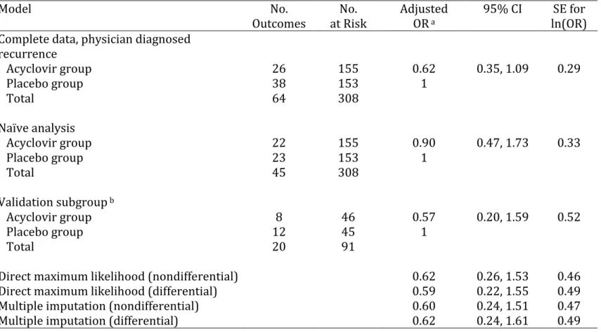
participants in the multicenter Herpetic Eye Disease Study followed for 12 months between 1992 – 1998 ... 61 Table 4.2. Estimates of the odds ratio comparing recurrence of ocular herpes

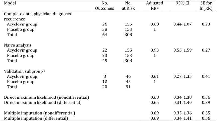
simplex virus between participants randomized to acyclovir or placebo from various models, 308 participants in the multicenter Herpetic Eye Disease Study followed for 12 months between 1992 – 1998 ... 62 Table 4.3. Estimates of the risk ratio comparing recurrence of ocular herpes

simplex virus between participants randomized to acyclovir or placebo from various models, 308 participants in the multicenter Herpetic Eye Disease Study followed for 12 months between 1992 – 1998 ... 63 Table 4.4. Bias and 95% confidence interval coverage for simulation

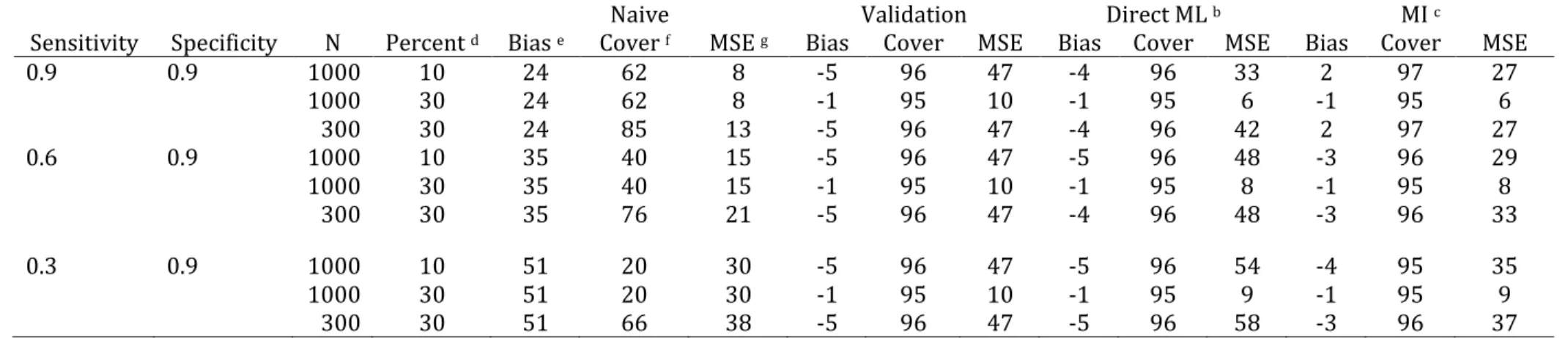
studies a_{under 9 scenarios for nondifferential misclassification ... 64}

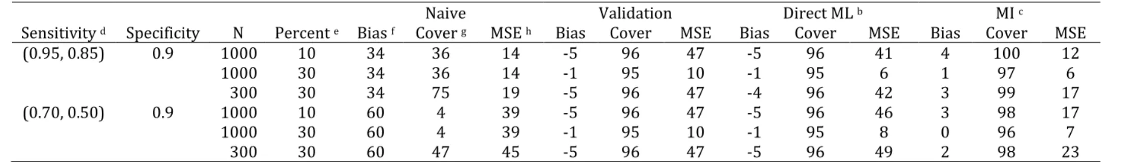
Table 4.5. Bias and 95% confidence interval coverage for simulation studies a_{under 6 scenarios for differential misclassification. ... 65}

Table 5.1 Characteristics of 3072 textile workers in South Carolina, United States, 1940 – 2001 ... 84 Table 5.2 Rate ratio of lung cancer mortality per 100 fiber-years/mL

cumulative asbestos exposure, South Carolina, United States, 1940 – 2001, under several outcome misclassification scenarios ... 85 Table 5.3 Rate ratio of lung cancer mortality per 100 fiber-years/mL

cumulative asbestos exposure, South Carolina, United States, 1940 – 2001, under several independent prior distributions

reflecting beliefs about outcome misclassification ... 86 Table A.1:Results accounting for outcome misclassification using Poisson

regression in 10,000 simulated cohorts a_{... 110}

(9)

ix

(10)

x

List of Figures

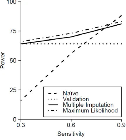
Figure 1.1. Example of a completed cause of death section on a US death certificate ... 24 Figure 4.1. Relationship between statistical power and sensitivity of the observed outcome measure in simulations with a 30% validation subgroup and a total sample size of 1000 for the naïve analysis, analysis limited to the validation subgroup, the direct maximum

(11)

xi

List of Abbreviations

CI Confidence interval

HEDS Herpetic Eye Disease Study HSV Herpes simplex virus MI Multiple imputation

ML Maximum likelihood

OR Odds ratio

PI Posterior interval

(12)

1 Background

The goal of many epidemiologic studies is to obtain an accurate estimate of the effect of an exposure on the occurrence of an event of interest. Measurement bias, selection bias, and confounding are three types of systematic errors that threaten the validity of results from epidemiologic studies. Selection bias and confounding are often considered in analysis of epidemiologic data, but the possible biases arising from measurement error are more routinely ignored.

Two problems occur in studies that disregard the potential for systematic bias: point estimates may be biased and uncertainty about the degree of systematic bias is not quantified. Most epidemiologic studies ignore the potential bias in point estimates and present some quantification of random error, such as the confidence interval, as the sole indicator of uncertainty in their results, ignoring the additional uncertainty that arises from systematic error. This systematic error is often more substantial than random error in large epidemiologic studies that are increasingly common (1,2).

(13)

2

This work begins by describing outcome misclassification, illustrating its potential to cause bias in two distinct types of epidemiologic studies, and describing existing

approaches to account for outcome misclassification. Chapter 2 outlines the specific aims of the proposed work, while chapter 3 details two proposed methods to account for outcome misclassification. Chapters 4 and 5 present results from the implementation of these methods in two settings, and chapter 6 summarizes the findings and offers discussion of the results.

1.1 Overview of outcome misclassification

Consider the two-by-two table of binary observed and true outcome measurements, W and D, respectively:

W=1 W=0

D=1 a b

D=0 c d

Using this notation, sensitivity, or the probability of being observed to be a case given that a participant is a true case, is defined as , and can be calculated from the table above as . Specificity, the probability of being observed to be a non-case given that a participant is actually not a case, is similarly defined as , and can be calculated from the table above as .

Sensitivity and specificity allow an investigator to hypothesize about the

(14)

3

of the data and a guess about the values of sensitivity and specificity. For example, one can calculate the expected probability of a participant’s being observed to experience the outcome, , in a study with specific values of sensitivity (se) and specificity (sp) and a known probability of experiencing the outcome, , using the equation:

.

In practical applications, however, investigators often have knowledge only about the observed data (i.e., and , or the margins and in the table above) and wish to make inferences about the true distribution of the outcome variable, and (the margins a + b and c + d in the table above).

To do this, investigators need information about the positive predictive value (PPV) and negative predictive value (NPV) of the observed outcome variable. The positive

predictive value is the probability that true outcome occurred, given than investigators observed the outcome to occur, . Assuming full knowledge of the two-by-two table above, this probability can also be calculated as . Similarly, the negative predictive value is the probability that a participant was not a case, given that he or she was not observed to experience the outcome, or . With full knowledge of the two-by-two table above, the negative predictive value could be calculated as .

An investigator can estimate the true probability of the outcome using the observed probability of the outcome and the positive and negative predictive values (PPV and NPV) through the formula

(15)

4

main study with the possibly misclassified outcome. Sensitivity and specificity are more widely-reported measures of outcome validity because these parameters are functions only of the outcome misclassification process. Positive and negative predictive values depend on the sensitivity and specificity of the observed outcome measure, but also on the prevalence of the outcome in the study population. To see this, consider how sensitivity and specificity can be related to positive and negative predictive value using Bayes’ Theorem:

which can be simplified to

where represents the P(D = 1) or the disease prevalence.

1.1.1 Differential and nondifferential outcome misclassification

Sensitivity and specificity of the outcome measure can be uniform over the entire study population or can differ by levels of exposure or other covariates. Consider the 2 by 2 table presented above stratified by exposure level to produce a 2 by 2 by k table, where k is the number of exposure levels.

X=1 X=0

W=1 W=0 W=1 W=0

D=1 a b D=1 a b

D=0 c d D=0 c d

(16)

5

Sensitivity and specificity are said to be nondifferential with respect to exposure X if and are the same for all possible values of

X. Outcome misclassification is said to be differential with respect to exposure status when

values of sensitivity and specificity differ across levels of exposure X. Because the positive and negative predictive values are functions of the prevalence of the outcome, they can differ within levels of exposure even with outcome misclassification is nondifferential with respect to exposure status (10).

1.1.2 Types of bias caused by outcome misclassification

Outcome misclassification can cause several distinct problems in epidemiology. First, outcome misclassification can cause errors in the overall estimation of outcome incidence or prevalence. If sensitivity of the observed outcome measure is less than 1, then false negatives can occur, in which a participant truly experiencing the outcome of interest is recorded not to have had the outcome. In specificity of the observed outcome measure is less than 1, false positives can occur, in which a participant who does not experience the outcome of interest is recorded to have the outcome. If more false negatives occur than false positives, the overall probability of the outcome will be underestimated. If more false positives occur, the probability of the outcome will be overestimated. Overall, imperfect sensitivity and specificity will cause error in the estimated incidence or prevalence of disease unless the number of false positives is exactly equal to the number of false negatives. Error in the marginal probability of the outcome causes bias not only in

(17)

6

Error in disease trends is compounded with the misclassification probabilities, sensitivity and specificity, also change over time (11).

Outcome misclassification can also cause bias in estimates of the effect of an exposure variable on an outcome. When outcome misclassification is nondifferential with respect to exposure and the outcome is binary, bias in estimates of the effect of the

exposure on the outcome is usually expected to be towards the null. However, this rule does not hold when the outcome has more than two levels or errors in exposure and outcome are not independent of each other (10,12–15). When outcome misclassification is differential with respect to exposure status, bias in estimates of the effect of the exposure on the outcome could be in either direction.

1.1.3 Methods for assessing the probability of misclassification

If a gold-standard measure of the outcome exists, investigators wishing to assess the amount of misclassification in a study may choose to conduct an internal validation study. In this type of study, the gold-standard outcome measurement is taken on a (possibly stratified) random subset of study participants. The gold-standard outcome measure is compared to the fallible outcome observed in the original study to calculate the sensitivity and specificity of the observed outcome measure.

(18)

7

Sensitivity and specificity from both internal and external validation studies will only accurately reflect the amount of misclassification in the main study if the relationship between gold-standard outcome and observed outcome is transportable between the validation study and the main study. Transportability implies that misclassification parameters are the same in the validation study and the main study, and would be expected for an internal validation study consisting of a random subgroup of the main study (16). Transportability is not assured for external validation studies or internal validation studies that are not a random subgroup of participants. In both situations, the validation study could represent a group of participants with characteristics different from participants in the main study. External validation studies carry the additional risk of nontransportability if the observed outcome measurement in the validation study was conducted differently from the observed outcome measurement in the main study.

1.2 Error in participant-reported outcomes

The outcome could be recorded with error for a variety of reasons, and the

opportunity for outcome misclassification arises throughout the study. This work focuses on two common types of outcome misclassification in epidemiology: error in participant-reported outcomes and misattribution of cause of death on death certificates, leading to misclassification of cause-specific mortality outcomes.

(19)

8

also known as patient-reported outcomes, a term which has evolved to include “any endpoint derived from patient reports, whether collected in the clinic, in a diary, or by other means, including single-item outcome measures, event logs, symptom reports, formal instruments to measure health-related quality of life, health status, adherence, and

satisfaction with treatment.” (20) These types of patient-reported outcomes have been used extensively in drug effectiveness research since the 1990s. Willke (20) reports that 30% of drug product labels approved between 1997 and 2002 used patient-reported outcomes as effectiveness study endpoints.

Recording outcomes described by participants is especially useful when time and cost constraints make frequent contact with investigators or physicians difficult or

impractical. In such situations, investigators may have contact with the participant at study enrollment and either at the end of the study period or at the end of pre-defined intervals of time, at which point the participant reports any events of interest occurring during the study period or interval. In these settings, participants may be instructed to keep a diary of outcome events on a daily or weekly basis. In other settings, a participant may be contacted by the investigator at only one point in time, at which time the investigator will ask the participant to recall events of interest in his or her past.

Opportunities for bias arise in all study designs using participant-reported outcomes. A prospective study, in which the participant is aware of being under

(20)

9

also subject to bias if participants fail to remember past events or inflate their number of past events.

Participants may misreport their outcomes due to errors in recall or due to social pressure to report one outcome over another. This social desirability bias arises most often when the outcome of interest is something within the direct control of the participant, such as a behavior, or when the outcome is taboo or embarrassing.

If participants in a prospective study do not know their exposure status, such as in a masked randomized trial, the outcome misclassification from under- or over-reporting symptoms or events of interest is likely to be nondifferential with respect to exposure. This means that the probability that a participant reports an event that occurred during the study period and the probability that a participant falsely reports an event that did not occur during the study period are not different for participants with different exposure values. In a masked randomized trial in which the participant does not know his or her exposure status, exposure is not likely to affect the participant’s reporting of the outcome. Because the probability of misclassification is the same for exposed and unexposed groups, effect estimates for binary outcomes subject to nondifferential misclassification are usually biased towards the null.

However, if participants in the prospective study do know their exposure status, outcome misclassification may be differential with respect to exposure. This means that exposed participants may be more or less likely to report an event that actually occurred or falsely report an event that did not occur than their unexposed counterparts. When

(21)

10

Differential outcome misclassification is even more likely in retrospective studies using participant-reported outcomes. When participants are asked to recall prior instances of events or symptoms, it is possible that participants who were exposed are more likely to remember events of disease than participants who were not exposed. For example, a mother living in a city blanketed in smog may be more likely to remember respiratory illnesses in her children than a mother living in an area with no smog, even if the children had similar respiratory histories. Differential outcome misclassification in retrospective studies is similar to recall bias in case control studies, in which cases are more likely to remember exposures than controls even with no association exists between exposure and outcome (21).

1.2.1 Herpetic Eye Disease Study

As an illustrative example, this work addresses outcome misclassification due to errors in participant-reported information in the Herpetic Eye Disease Study, a randomized trial of acyclovir for preventing ocular herpes simplex virus (HSV) recurrence. Ocular HSV infection can cause corneal opacities and vision loss (22), and at least 500,000 people in the United States are infected (23). Treatment of HSV is estimated to cost approximately $17.7 million annually to treat about 59,000 new and recurrent cases (24).

Recurrent infections are a major contributor to vision loss from ocular HSV. After an initial (usually asymptomatic) infection, HSV establishes a latent infection in the trigeminal or other sensory ganglia. From these locations, recurrent viral shedding can lead to

(22)

11

membrane lining the eyelids, or dendritic or epithelial keratitis, characterized by a linear branching corneal ulcer. Infection can also lead to stromal keratitis, causing inflammation of the cornea, or iritis, causing inflammation of the anterior uvea, both of which can lead to permanent scarring and decreased vision.

The primary objective of the Herpetic Eye Disease Study was to determine whether treatment with oral acyclovir for one year would prevent ocular recurrences in

participants who had had an episode of ocular HSV during the preceding year (22). The outcome of interest in the trial was ocular HSV recurrence diagnosed by an experienced ophthalmologist using slit lamp biomicroscopy. HSV recurrence was assessed after 1, 3, 6, 9, and12 months of treatment; during the post-treatment observation period, after months 13, 15, and 18; and any time new ocular symptoms developed.

However, a companion cohort study was also performed, nested within the

randomized trial of acyclovir, to assess psychological stress and other triggers of recurrent HSV infection. In this companion study, HSV recurrence was assess both by an experienced ophthalmologist and through participant self-report in weekly diaries (25). Participants were instructed to record the date of the onset of symptoms of HSV recurrence. Such symptoms included redness and swelling of the eye, blurred vision, sensitivity to light, inflammation of the eyelids, or the sensation of a foreign object in the eye.

(23)

12

weekly diaries remain subject to outcome misclassification due to factors such as social desireability and lack of medical training to identify events of interest.

This work uses the Herpetic Eye Disease Study and its companion study of triggers of recurrence to explore methods to account for outcome misclassification in a setting with both gold standard (physician diagnosis) and error-prone (weekly diary) outcome measure available.

1.3 Misattribution of cause of death

In addition to accounting for outcome misclassification of participant-reported outcomes, this work focuses on accounting for misclassification of cause-specific mortality outcomes caused by misattribution of cause of death.

(24)

13

or nonmalignant disease causes a spurious increase in survival of those diagnosed as cases (31).

Before the introduction of the national death index in the United States in 1978, vital status was determined in epidemiologic studies by examining sources such the US Social Security Administration, Internal Revenue Service, state vital statistics office, drivers’ license files, and US postal service change of address forms. After 1978, vital status was recorded centrally in the National Death Index, a computerized index of death record information on file in state vital statistics offices. For all deaths identified using any of these sources, cause of death is typically abstracted from death certificates, and these causes of death are used to assign outcome statuses to participants in epidemiologic studies.

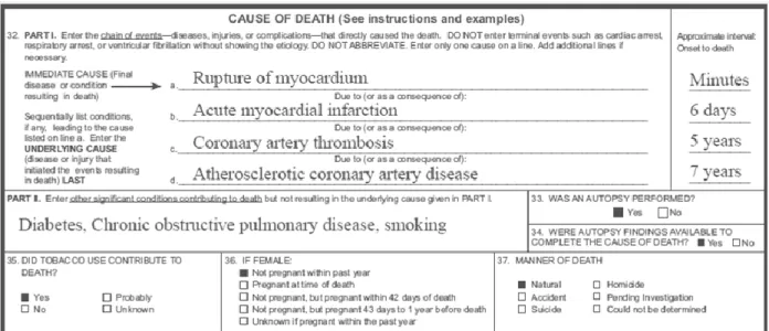
Cause of death information on the death certificate is typically completed by a

physician, medical examiner, or coroner. Figure 1.1 presents the cause of death section on a United States death certificate. In part 1, the physician, medical examiner, or coroner is instructed to report the chain of events leading to directly death, with the immediate cause of death listed first and the underlying cause of death listed last. Part 2 captures all other significant diseases, conditions, or injuries that contributed to death but did not result in the underlying or immediate cause of death. The cause of death reflects the best medical opinion of the person filling out the death certificate and does not need to be supported by a definitive diagnosis in a medical setting.

(25)

14

participants with ICD codes from the cause of death on death certificates matching these ICD codes are designated to have the event of interest. Studies of the reliability and

accuracy of cause of death information reported by physicians have revealed that the same patient reviewed by different physicians is likely to be assigned different causes of death (32).

Because coroners responsible for certifying the underlying cause of death may receive limited medical training as well as the uncertainty inherent in ascribing cause of death for some conditions, underlying cause of death reported on death certificates is error-prone. Misattribution of underlying cause of death has plagued epidemiologic studies of cause-specific mortality (33,34). Studies of etiologic relationships between exposures and cause-specific mortality as well as studies assessing secular trends of cause-specific mortality are subject to bias due to outcome misclassification caused by misattribution of underlying cause of death.

Because misattribution of underlying cause of death can lead to outcome

misclassification, cause-specific mortality outcomes abstracted from death certificates have imperfect sensitivity and specificity. Recall that sensitivity is the probability of a true case being classified as such; and specificity is the probability that a true non-case being

classified as such. Using autopsy data as a gold standard, sensitivity and specificity of cause of death information from death certificates is imperfect even for well-studied and

(26)

15

(27)

16

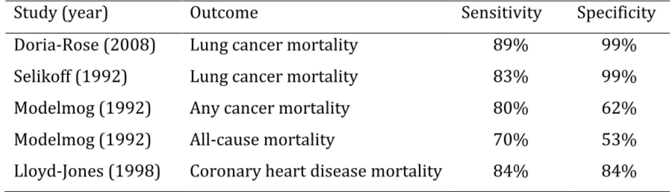
Table 1.1: Sensitivity and specificity estimates of cause-specific mortality from the literature.

1.3.1 Misattribution of underlying cause of death in occupational cohort studies

Many cohort studies of occupational exposures have used cause-specific mortality as an outcome measure. Cause-specific mortality is often chosen over disease incidence as an outcome measure for practical reasons. Workers are usually enrolled at some point during their employment, at which time their exposure history is recorded for the duration of their employment, along with other relevant covariates. However, the diseases of

interest affecting these workers typically occur later in life, at which time few are likely to be working. Because date and cause of death can be identified using publically available information from the National Death Index and death certificates, investigators can identify cause-specific mortality outcomes without performing extensive follow-up on each worker. Like all studies using cause of death abstracted from death certificates, occupational cohort studies of cause-specific mortality are subject to bias due to outcome

misclassification caused by misattribution of underlying cause of death.

Study (year) Outcome Sensitivity Specificity

Doria-Rose (2008) Lung cancer mortality 89% 99%

Selikoff (1992) Lung cancer mortality 83% 99%

Modelmog (1992) Any cancer mortality 80% 62%

Modelmog (1992) All-cause mortality 70% 53%

(28)

17

1.3.2 Misattribution of cause of death in the South Carolina textile workers study This work assesses the impact of misattribution of cause of death in the

occupational setting using data from a study of workers exposed to asbestos at a South Carolina textile factory. “Asbestos” is the generic name given to a group of naturally occurring silicate minerals with fibrous structure that became commonly used as an insulator for both electrical wires and buildings due to its heat and flame resistant properties after the industrial revolution. Industrial production of asbestos began in the 1850s, and, due to its attractive fire-resistant properties, asbestos was eventually

incorporated into many building materials, such as bricks, concrete, pipes, ceiling insulation, drywall, flooring, and roofing materials. However, by the middle of the 20th

century, asbestos exposure had been shown to increase the risk of both malignant and non-malignant lung diseases (38).

(29)

18

including Brazil, India, China and Russia. Therefore asbestos continues to pose important occupational hazards in the US and worldwide (41).

Epidemiologic studies have shown a relationship between exposure to asbestos and lung cancer mortality, though the carcinogenic mechanism is not fully established. The two major types of asbestos fibers are chrysotile fibers and amphiboles, including actinolite, amosite, anthrophyllite, crocidolite, and tremolite (42). Amphibole fibers are more carcinogenic than chrysotile in part because they are more biopersistent in the lung

(amphiboles have an estimated half-life in the lungs of decades, while chrysotile fibers have a half-life of months (38)), accumulate in the distal lung parenchyma, and are not cleared as easily. However, both fiber types can induce DNA damage, gene transcription, and protein expression important to modulate cell proliferation and cell death in bronchial and alveolar epithelial cells (43). When asbestos fibers reach the lungs, alveolar epithelial cells and alveolar macrophages internalize the fibers, resulting in oxidative stress and the

subsequent generation of reactive oxygen species and reactive nitrogen species, which can cause DNA damage.

(30)

19

exposed only to the chrysotile form of asbestos had been conducted. However, like all studies relying on cause of death information from death certificates, estimates from the study of South Carolina textiles workers are subject to bias due to outcome

misclassification from misattribution of cause of death.

Unlike the Herpetic Eye Disease Study, no internal gold standard outcome is available for participants in the South Carolina textile workers cohort. In other cohorts, limited validation studies have been performed comparing lung cancer and coronary heart disease mortality reported on death certificates to lung cancer deaths and deaths due to coronary heart disease identified through autopsies and physician diagnosis.

The Life Span Study, which performed autopsies on selected participants who died following the atomic bombings of Hiroshima and Nagasaki, found that death certificates detected that a death was due to lung cancer in only 62% of the cases where the autopsy indicated that lung cancer was the cause of death (36). A more recent study from the Mayo lung clinic in the United States reported that death certificates identified lung cancer as the cause of death in 89% (210/237) of autopsy-confirmed lung cancer cases (34), while specificity was 99%. Sensitivity from other validation studies fell between the estimates from the Life Span Study and the Mayo lung clinic. A study of 4951 deaths occurring among 17,800 workers exposed to asbestos reported that death certificates identified lung cancer as the cause of death in 86% of the deaths designated as lung cancer deaths by autopsy and other medical evidence (37).

(31)

20

1.4 Existing methods to account for outcome misclassification

1.4.1 Algebraic approaches

Approaches to account for bias in crude effect estimates due to use of a misclassified binary outcome variable have existed for more than half a century (44). These approaches use simple bias correction formulas to account for misclassification in two-by-two tables. In these approaches, “true” counts of outcomes in each strata of exposure are predicted from the observed number of outcomes and given values of sensitivity and specificity.

Algebraic approaches to account for outcome misclassification can be deterministic (44) or probabilistic (10,45). Both types of algebraic methods to account for

misclassification can be used as part of a sensitivity analysis in which the investigator evaluates the changes in the point estimate of the effect of the exposure on the outcome due to different hypothesized values for sensitivity and specificity. The probabilistic

analysis offers an advantage in that it also provides a means to assess the uncertainty in the final point estimates due to outcome misclassification (10).

1.4.2 The EM algorithm

More recently, investigators have developed maximum likelihood approaches for logistic regression to produce effect estimates accounting for outcome misclassification while adjusting for relevant confounders (46,47).

(32)

21

investigators perform standard logistic regression considering each individual as both diseased and non-diseased with weights determined by the probability that the study subject is truly diseased given the data. Specifically, for individuals designated as cases by the error prone outcome indicator (Wi=1), the probability that the individual is truly

diseased is the predicted value of a positive test for that individual calculated from the covariates, regression coefficients, sensitivity, and specificity using Bayes’s Theorem. For individuals designated as non-cases by the error prone outcome variable (Wi=0), the

probability that the _{individual is truly diseased is the predicted positive value of a} negative test. Because the probabilities depended on regression parameters, they are recalculated after the logistic regression parameters are estimated, which leads to new probabilities and thus, new regression parameters. The processes of estimating the probabilities and the logistic regression parameters are repeated alternately until the parameter estimates converge.

This method can account for differential outcome misclassification (with respect to exposure or covariates) by assigning different values of sensitivity and specificity to individuals with different sets of values for exposure or covariates. This method can also incorporate internal validation data to estimate sensitivity and specificity.

1.4.2 Direct maximum likelihood

(33)

22

external or internal validation data, the sensitivity and specificity are estimated from the data based on specified covariates. It can also be extended to the case control setting when internal validation data are available (47).

The direct maximum likelihood approach for a main study with a validation subgroup specifies the likelihood for the logistic regression model relating exposure to outcome as the product of the likelihood for the main study and the likelihood for the validation subgroup. In both likelihood terms, sensitivity and specificity are based on associations between observed outcome, gold standard outcome, and exposure defined using a logistic model

logit[ ] for Sensitivity and specificity are calculated as

and

The likelihood for the main study is then modified by the estimated values of sensitivity and specificity for each observation and multiplied by the likelihood for the validation study. Lyles (47) presents approaches to account for outcome misclassification in situations with internal validation data, external validation data, and assumed values of sensitivity and specificity.

The direct maximum likelihood approach applied to account for outcome

(34)

23

]

And in the log binomial model,

]

1.5 Summary

Outcome misclassification is a neglected problem in epidemiologic research despite common use of study endpoints subject to measurement error. Several methods exist to account for misclassification of binary outcomes, but these methods are not

(35)

24 Figures

(36)

2 Specific Aims

Misclassification of outcome variables is a threat to the accuracy of epidemiologic studies. Outcome misclassification occurs when investigators observe an error-corrupted version of the event of interest instead of the true outcome status of study participants. Both binary event indicators and continuous outcomes are subject to misclassification, but standard approaches to analyzing cohort data typically assume such biases are absent.

Outcome misclassification can occur in many settings, but this work focuses on two specific types of error in outcome measurements: misclassification due to incorrect

information reported by study participants and misattribution of cause of death on death certificates leading to outcome misclassification in mortality studies. This work develops methods to account for outcome misclassification in diverse situations both with and without validation data and in both binary regression models and time-to-event analyses.

(37)

26

of acyclovir on herpes recurrence that are not biased by incorrect outcome information supplied by participants.

(38)

3 Methods

This thesis focuses on three methods to account for outcome misclassification in a range of epidemiologic settings: multiple imputation, maximum likelihood, and Bayesian analysis. The principle features of the methods are described below, and specific

applications of the methods are detailed in chapter 4 (multiple imputation) and chapter 5 (maximum likelihood and Bayesian analysis).

3.1 Multiple imputation to account for outcome misclassification

This work begins by describing the use of multiple imputation to address outcome misclassification in studies with internal validation data. Multiple imputation is a standard technique for handling missing data (50,51). We use multiple imputation to account for outcome misclassification by viewing outcome misclassification as a missing data problem.

(39)

28

efficient as ) if X is missing at random within strata of Z.Missing at random implies that missingness of X may depend on Z but not on X itself (after controlling for Z) (52).

In a study with an internal validation subgroup, the possibly misclassified outcome (W) is available for all participants, but the gold-standard outcome (D) is available only for participants in the validation subgroup. If participants are selected into the validation subgroup randomly within strata of exposure (X) and covariates (Z), information on the gold-standard outcome can be said to be missing at random in the full cohort. The missing at random assumption allows us to exploit the relationships between D, W, X, and Z among participants in the validation subgroup to impute values for D for all other participants.

To account for outcome misclassification using multiple imputation, we use the logistic method for monotone missing data (53). As a first step, the gold-standard outcome D is regressed on the possibly misclassified outcome W, the exposure X, and other relevant

covariates Z in the validation subgroup using the logistic regression model shown in Equation 3.1.

3.1

Regression parameters are assumed to follow a multivariate Gaussian distribution with mean vector ( ̂ ̂ ̂ ̂ ̂ and covariance matrix ( ̂ estimated from the logistic regression model above. Regression parameters are drawn for each of K

(40)

29

A new variable, , is created to represent the imputed outcome, where k indexes the number of imputations. By definition, = D for participants in the validation

subgroup. For participants not in the validation subgroup, is imputed based on

regression coefficients drawn for each imputation. For each imputation, is assigned by a random draw from a Bernoulli distribution with probability , where

3.2 ( ̂ ̂ ̂ ̂ ̂ )

( ̂ ̂ ̂ ̂ ̂ )

At this point in the analysis, K datasets exist with imputed outcomes for all participants. The relationship between exposure and outcome in these datasets can be analyzed with any type of analysis model desired. For example, to estimate the risk ratio for the effect of exposure X on true outcome D,

we can use binomial regression to estimate the effect of exposure X on the imputed

outcome in each of the K datasets. The binomial model for the imputed outcome given the exposure and relevant covariates for k = 1, 2, … , K is

3.3 ( )

The estimated risk ratio from this model is ( ̅ ) ( _∑ _̂

), where ̂ is the natural log of the estimated risk ratio from the kth_{imputed dataset. The variance for ̅} _is

(41)

30

3.4 ( ̅ ) ∑ ̂( ̂ ) ( ) (

) ∑( ̂ ̅ )

The choice of effect measure is flexible. For example, if one wished to estimate the odds ratio in place of the risk ratio

logistic regression could be used as the analysis model in place of log binomial regression. The logistic models for the imputed outcome given treatment group and relevant

covariates for k=1 to K are

3.5

and the odds ratio is given by is ( ̅ ) ( _∑ _̂

), where ̂ is the natural log of the estimated odds ratio from the kth_{imputed dataset. Variance is again computed using}

equation 3.4.

Regardless of the choice of effect estimate, the analysis model need not match the imputation model. Covariates likely to influence the outcome misclassification process may be used in the imputation model (3.1) but excluded from the analysis model if they do not meet the criteria for covariate inclusion in the analysis model. Addition of covariates to the imputation model rarely reduces the precision of the final estimate, and any decline in precision is generally offset with a reduction in bias (51).

The imputation model shown in Equation 3.1 can be used to account for outcome misclassification that is differential or nondifferential with respect to exposure.

(42)

31

assesses the outcome does not have knowledge of the participants’ exposure status. The assumption of nondifferential misclassification implies that in the imputation model shown in Equation 3.1. In models where is allowed to be different from 0, separation of data points can occur if the size of the validation subgroup is small. Firth’s correction (54) can be applied in these settings to prevent separation of data points (55). Firth’s correction uses a modified score function to obtain maximum likelihood estimates when response variables can be perfectly predicted by a linear combination of risk factors (55), a situation known as separation (56) or monotone likelihood (57). Firth’s correction may be viewed as a multivariable extension of a continuity correction.

3.2 Maximum likelihood to account for outcome misclassification

The following section discusses the use of modified maximum likelihood to account for outcome misclassification. In this section, we assume no validation data are available and perform sensitivity analyses by setting values of sensitivity and specificity.

The maximum likelihood approach to account for outcome misclassification in logistic regression was outlined by Lyles (47). Briefly, for a logistic regression model comparing the odds of outcome between exposure groups X controlling for covariates Z,

[ ] ∑

each independent record i contributes the following likelihood term

3.6

(43)

32

If a misclassified version of the outcome variable, W, is observed in place of the gold standard outcome Y, the estimated odds ratio is subject to bias. To account for outcome misclassification in the logistic model, the likelihood is rewritten in terms of W, sensitivity, and specificity.

3.7 [ ] [

]

Here, we extend this approach to account for outcome misclassification due to misattribution of cause of death. When outcome misclassification is thought to be

attributable only to misspecification of the cause of death, several issues emerge. First, the dates of death are assumed to be correct. Second, participants alive at the end of the study are not subject to outcome misclassification. Similarly, the misclassification probabilities apply only to deaths observed to occur during the study.

We choose to study the relationship between cause-specific mortality and an exposure of interest using Poisson regression. When estimating the rate ratio of death due to cause A per unit increase in exposure X using Poisson regression, the parameter

estimating the desired rate ratio is in the Poisson model below,

3.8

( ∑

)

where represents the rate of death due to cause A in strata j, Xj is the exposure, and Z is a

matrix with columns for each of covariates in the model.

(44)

33

continuous exposures or covariates, these variables must be categorized. Each strata contains a count of the number of person years contributed to that strata ( and the number of deaths . In each strata, deaths are attributed to the cause of interest (cause ), though the true number of deaths due to cause is unobserved. The true number of person-years and deaths remains nj and dj, respectively, under the assumption

that the dates of death are correct.

Under the ideal model specified above, the likelihood expression would be

3.9 ∏ ( )

The first term , captures the number of events occurring in strata j, and the second term, ( ) takes the number of person-years contributed in strata j into account.

However, because we observe wj possibly misclassified deaths due to cause in place

of true deaths due to cause , the model above cannot be fit directly. Instead, standard analyses typically fit the model

( ∑

)

where represents the rate of a possibly misclassified version of the outcome variable, wj

and represents an estimate of the rate ratio possibly biased by outcome misclassification.

(45)

34

3.10 ∏ ( )

where is described above, , , and is the estimated rate of deaths due to causes other than cause A for strata j,

( ∑

)

where Z is a matrix with columns for the L covariates included in the analysis. As in the likelihood function for one cause of death, deaths due to cause A contributed to the first term, , deaths due to other causes contributed to the second term, , and person-time is taken into account in the third term, ( ) .

Because the true number of deaths due to cause A is unavailable, the likelihood is modified to use the count of potentially misclassified deaths due to cause A for each stratum, and the misclassification probabilities (i.e., sensitivity and specificity) to restructure the likelihood as:

3.11

∏ { } { }

exp [ ] .

(46)

35

performed by setting sensitivity and specificity to plausible values identified using the existing literature or through expert opinion.

3.3 Bayesian analysis to account for outcome misclassification

The sensitivity analysis approach outlined above requires the investigator to set the value of sensitivity and specificity. When an investigator suspects outcome

misclassification is present based on external validation studies or expert opinion, Bayesian methods offer an appealing alternative to sensitivity analysis.

Uncertainty about the amount of misclassification in the data can be acknowledged explicitly by placing informative prior distributions on sensitivity and specificity that reflect beliefs about the amount of misclassification in the data and certainty about those beliefs. Bayes’s theorem offers a method to combine these prior probability distributions for sensitivity and specificity with the observed data characterized by likelihood function 3.6 to obtain a posterior distribution of the parameter(s) of interest. In this case, the parameter of interest is from model 3.9. Non-informative, null-centered priors are placed on the regression parameters.

(47)

36 3.4 Application to the Herpetic Eye Disease Study

We implement the multiple imputation approach to account for outcome

misclassification due to error in participant reported outcomes in the Herpetic Eye Disease Study. The Herpetic Eye Disease Study is a randomized trial of acyclovir for preventing ocular herpes simplex virus (HSV) recurrence at 58 university and community-based sites in the United States (22). Participants were 12 years of age and older and had an episode of ocular HSV in the 12 months before the study, but their disease had been inactive during the 30 days preceding the study. During the study, the 703 participants were randomized to receive either oral acyclovir or placebo. The acyclovir group received 400 mg of

acyclovir twice daily for 12 months, and the placebo group received oral placebos with the same frequency. The goal of the study was to compare the 12-month incidence of ocular HSV recurrence between the group randomized to receive acyclovir and the group

randomized to receive placebo. Information was collected on age, race, gender, and number of ocular recurrences prior to randomization. Participants returned for five follow-up visits during the one-year treatment period and an additional three follow-up visits during the six months immediately following the treatment period. HSV recurrences that were diagnosed during the trial were treated with topical corticosteroids and antivirals, though oral acyclovir or placebo was continued for the duration of the one-year treatment period.

(48)

37

chronic stressors, including illnesses, injuries, menstrual periods, sun exposure, and emotional and financial stresses. This analysis was limited to the 308 Herpetic Eye disease study patients who also enrolled in the recurrence factors study.

The outcome of interest was a binary indicator of HSV recurrence over the 12-month study period. Among participants in the recurrence factors study, HSV recurrence was assessed in two ways. First, participants recorded symptoms of HSV recurrence in their weekly diaries. In addition, study-certified ophthalmologists examined participants using microscopy when symptoms were apparent or at planned study visits in months 1, 3, 6, 9, and 12. This analysis will consider physician-diagnosed ocular recurrence to be the gold-standard outcome measure, represented by D, and participant-reported symptoms to be the error-prone outcome measure, represented by W.

The effect of interest was the odds ratio comparing the incidence of HSV recurrence among participants randomized to receive acyclovir to incidence of HSV recurrence among participants randomized to placebo. The first analysis was conducted using physician-diagnosed HSV recurrence as the outcome measure on all participants. The odds ratio was estimated as in the logistic regression model

where D represents physician-diagnosed recurrence, X is treatment assignment to acyclovir (X = 1) or placebo (X = 0), and Z is a vector of covariates including age, sex, and number of previous recurrences.

To assess the performance of multiple imputation to account for outcome

(49)

38

the 308 participants in the recurrence factors study. Participant-reported symptoms of HSV recurrence (W) was assumed to be available for all participants, but physician-diagnosed HSV recurrence was assumed to be available only for participants randomly selected to be in the validation subgroup. Thus, the hypothetical validation subgroup mimicked an internal validation subgroup randomly sampled from the main study.

We compared results of an ideal analysis on the full cohort of 308 participants using the physician diagnosis as the outcome variable with results from four methods for

handling outcome misclassification: 1) the naïve analysis, in which participant-reported outcome (W) represented the outcome status for all 308 participants; 2) the validation subgroup, in which the physician-diagnosed outcomes (D) were compared between those receiving acyclovir and those receiving placebo in the validation subgroup of 91

participants; 3) a direct maximum likelihood approach (47) to account for outcome misclassification and; 4) multiple imputation to account for outcome misclassification. Direct maximum likelihood and multiple imputation approaches were evaluated under the assumptions of both differential and nondifferential misclassification of the outcome with respect to treatment group.

3.5 Application to study of South Carolina textile workers study

(50)

39

employed at the plant for at least one month between 1 January 1940 and 31 December 1965. Employment records were used to obtain information on date of birth, year of study entry, race (Caucasian or non-Caucasian), sex, and employment status in each year.

Detailed work histories, including plant department, job held by the participant, and start and end dates, were available for each participant in the cohort. Cumulative exposure to the chrysotile form of asbestos was estimated using a job exposure matrix to link work history to industrial hygiene sampling measurements taken between 1930 and 1975, as previously described (59). Industrial hygiene data were collected from the company

insurance carrier, the State Board of Health, the US Public Health Service, and the company sampling program (58). Chrysotile exposure concentrations, expressed as fibers longer than 5 micrometers per milliliter of air (fibers/mL), were estimated for each day of each participant’s work history. Yearly exposure values were calculated as the product of the proportion of the year worked and the average daily exposure concentration and reported as fiber-years per milliliter (fiber-y/mL). To capture the appropriate exposure window for the effect of asbestos on lung cancer mortality, exposure values were lagged 10 years, meaning that the risk of lung cancer in each year was not affected by asbestos exposure in the prior 10 years. Chrysotile was the only type of asbestos ever processed at the plant as a raw fiber, indicating that confounding exposure by other types of asbestos figures, such as crocidolite, is unlikely.

(51)

40

traced using local telephone listings, property records, voter records, records of funeral homes, and other local sources (42).

Between 1979 and 2001, vital status was determined using the National Death Index. Those confirmed alive in 1979 and not found in the National Death Index were assumed to be alive at the end of the study. For those who died, cause of death was

determined through examination of death certificates and coded by a qualified nosologist into the revision of the International Classification of Diseases (ICD) in effect at the date of each death.

In this cohort, we estimated the effects of asbestos exposure on the rate of death due to lung cancer. A death was classified as a death due to lung cancer using ICD-7, ICD-8, and ICD-9 code 162. Cause of death reported on the death certificate was the error-prone version of the outcome variable, but, unlike the earlier example from the Herpetic Eye Disease Study, no internal validation subgroup was available to assess the possible outcome misclassification. To account for outcome misclassification, we performed sensitivity analysis using modified maximum likelihood and the Bayesian analysis placing informative prior distributions on sensitivity and specificity as described above. The effect of interest was the rate ratio of lung cancer death per 100 f-y/mL of asbestos exposure.

3.6 Simulations

(52)

41

size, effect size, misclassification parameters, and size of the validation subgroup, if applicable.

In each simulation experiment, the distribution of exposure was designed to mimic a real-data example. For example, in the simulations to evaluate multiple imputation to account for outcome misclassification, the exposure distribution reflected the distribution of acyclovir exposure in the Herpetic Eye Disease Study data. In the simulation experiments to assess the performance of modified maximum likelihood to account for outcome

misclassification, the exposure distribution was designed to mimic the distribution of asbestos exposures among participants in the South Carolina textile workers study.

True outcome variables were generated based on the exposure and effect size of interest. The effect size was varied across scenarios. In the simulations designed to assess the performance of multiple imputation, the true binary outcome indicator was generated directly from the exposure and effect size. In the simulations for maximum likelihood, the true time to death due to cause A was generated along with a true time to death due to all other causes. If the time to death due cause A was less than the time to death due to other causes, the death was a death due to cause A. Otherwise, the simulated participant was said to have died from other causes.

In each simulation, a misclassified version of the outcome variable was generated based on the true outcome variable and the values of the misclassification parameters. Values of sensitivity and specificity were altered for each simulated scenario.

(53)

42

cohorts mimicking the Herpetic Eye Disease study data) or modified maximum likelihood (for the cohorts mimicking the South Carolina textile workers study).

We assessed the performance of each method to account for outcome

misclassification by comparing bias, 95% confidence interval coverage, statistical power, and mean-squared error between the standard analysis with the analysis using multiple imputation or modified maximum likelihood to account for outcome misclassification. Bias was defined as 100 times the difference between the average estimated effect size and true effect size, and confidence interval coverage was calculated as the proportion of

(54)

4 Accounting for misclassified outcomes in binary regression models

using multiple imputation with internal validation data

Outcome misclassification is widespread in epidemiology, but methods to account for it are rarely used. We describe the use of multiple imputation to reduce bias when validation data are available for a subgroup of study participants. This approach is

illustrated using data from 308 participants in the multicenter Herpetic Eye Disease Study between 1992 and 1998 (48% female, 85% Caucasian, median age 49 years). The odds ratio (OR) comparing acyclovir and placebo groups on the gold-standard outcome

(physician-diagnosed herpes simplex virus recurrence) was 0.62 (95% confidence interval (CI): 0.35, 1.09). We discarded physician diagnosis except a 30% validation subgroup to compare methods. Multiple imputation (OR=0.60; 95% CI: 0.24, 1.51) was compared to naïve analysis using self-reported outcomes (OR=0.90; 95% CI: 0.47, 1.73), analysis restricted to the validation subgroup (OR=0.57; 95% CI: 0.20, 1.59), and direct maximum likelihood (OR=0.62; 95% CI: 0.26, 1.53). In simulations, multiple imputation and direct maximum likelihood had greater statistical power than analysis restricted to the validation subgroup, yet all three provided unbiased estimates of the OR. The multiple imputation approach was extended to estimate risk ratios using log-binomial regression. Multiple imputation has advantages regarding flexibility and ease of implementation for

(55)

44 4.1 Introduction

Misclassification of outcome variables is common in epidemiology and threatens the validity of inferences from epidemiologic studies (1,2). However, standard approaches to epidemiologic data analysis typically assume outcome misclassification is absent. Although approaches to account for bias in crude effect estimates due to use of a misclassified binary outcome have existed for more than half a century (46), these methods are rarely used because epidemiologists commonly wish to present results adjusted for several

confounding variables. More recently, investigators have developed maximum likelihood approaches (2,3) to produce odds ratio estimates that account for outcome

misclassification while adjusting for relevant confounders using logistic regression, but these methods have not been widely applied in the epidemiologic literature. Here we describe an alternative approach to account for outcome misclassification using missing data methods that are familiar to epidemiologists.

(56)

45

multiple imputation to estimate odds ratios and risk ratios, provide examples using cohort data (25), and explore some finite sample properties of the proposed method by Monte Carlo simulation.

4.2 Methods Study population

We illustrate the use of multiple imputation to account for outcome misclassification using data from the Herpetic Eye Disease Study, a randomized trial of acyclovir for

preventing ocular herpes simplex virus (HSV) recurrence at 58 university and community-based sites in the United States (22). Participants were 12 years of age and older and had an episode of ocular HSV in the 12 months before the study, but their disease had been inactive during the 30 days preceding the study. During the study, the 703 participants received either oral acyclovir or placebo for 12 months. The goal of the study was to

compare the 12-month incidence of ocular HSV recurrence between the group randomized to receive acyclovir and the group randomized to receive placebo. Information was also collected on age, race, gender, and number of ocular recurrences prior to randomization. Here, we restrict analyses to the 308 of 703 participants who co-enrolled in a study that collected weekly diaries about ocular HSV symptoms and possible triggers between 1992 and 1998(60).

Outcome Ascertainment and Validation

(57)

46

ophthalmologists examined participants using microscopy when symptoms were apparent or at planned study visits in months 1, 3, 6, 9, and 12. In addition, participant-reported HSV recurrence was obtained from a weekly diary. We consider participant-reported HSV recurrence to be the observed, and possibly mismeasured, version of the outcome variable ( if the participant reported any recurrence, otherwise), and physician-diagnosed HSV recurrence to be the gold standard (D = 1 if the ophthalmologist physician-diagnosed a recurrence, D = 0 otherwise). We randomly sampled 30% (n = 91) of the 308 participants to treat as a validation subgroup. In this analysis, we assume that W was available for all participants and D was observed only for those selected to be in this hypothetical

validation subgroup.

Statistical methods

(58)

47

and nondifferential misclassification of the outcome with respect to treatment group. We further extended the direct maximum likelihood and multiple imputation approaches to estimate risk ratios using log-binomial regression.

The direct maximum likelihood approach accounted for outcome misclassification using the method described by Lyles et al (47). This approach included data from all participants, with those in the validation subgroup providing data on the correctly classified outcome and those not in the validation subgroup providing data on the

misclassified outcome. In contrast, the naïve analysis included data from all participants, but used only the misclassified outcome, and the validation analysis included data from participants in the validation subgroup only, but used the correctly classified outcome. To account for nondifferential misclassification in the direct maximum likelihood approach, we estimated the sensitivity and specificity from the records in the validation subgroup. These values were used to compute the likelihood to be maximized, which was a product of the main study likelihood and the validation sample likelihood, as detailed in Appendix 1. To relax the assumption of nondifferential misclassification, we added treatment group to the model for sensitivity and specificity.

Multiple imputation is a standard technique for handling missing data (50,51). We use multiple imputation to account for outcome misclassification by exploiting the

relationships between D, W, treatment group (X), and other covariates (Z) among

(59)

48

we regress physician-diagnosed HSV recurrence (D) on participant-reported HSV

recurrence (W), treatment group (X), and other covariates (Z) using a logistic regression model

4.1

We then draw a set of regression coefficients for each of K imputations from the posterior predictive distribution of the parameters. We set K = 40 in this analysis. Assume parameters follow a multivariate Gaussian distribution with mean vector

( ̂ ̂ ̂ ̂ ̂ and covariance matrix ( ̂ estimated from the logistic regression model above. Drawing regression coefficients for each imputation allows uncertainty about the relationship between W, X, and D to propagate through the analysis (50).

A new variable, , is created to represent the imputed outcome. For participants in the validation subgroup, = , where k indexes the number of imputations. For

participants not in the validation study, values for are imputed based on the regression coefficients drawn for that imputation. For each imputation, is assigned by a random draw from a Bernoulli distribution with probability , where

4.2 ( ̂ ̂ ̂ ̂ ̂ )

( ̂ ̂ ̂ ̂ ̂ )

(60)

49

combine results using standard multiple imputation techniques (51). The logistic models for the imputed outcome given treatment group and relevant covariates for k=1 to 40 are

4.3

The estimated odds ratio is

4.4 ( ̅ ) ( _{∑ ̂}

)

where ̂ is the natural log of the estimated odds ratio from the kth_{imputed dataset. The}

variance for ̅ is given by

4.5 ( ̅ ) ∑ ̂( ̂ ) ( ) (

) ∑( ̂ ̅ )

In a closed cohort, it may be preferable to estimate the risk ratio instead of the odds ratio (61–63). To illustrate the ability of the proposed multiple imputation approach to estimate different parameters of interest, we also use a log-binomial regression model to estimate the risk ratio comparing imputed HSV recurrence for participants assigned to acyclovir and those assigned to placebo in each imputation. To estimate a risk ratio, the binomial model for the imputed outcome given treatment group and relevant covariates for k = 1 to 40 is used in place of the logistic model shown in Equation 4.3.

(61)

50

Multiple imputation can be used to account for misclassification of the outcome that is differential or nondifferential with respect to treatment group. The assumption of

nondifferential misclassification implies that in the imputation model (Equation

4.2). In models where was allowed to be different from 0, because the validation

subgroup was relatively small, we used Firth’s correction (54) to prevent separation of data points (55). Firth’s correction uses a modified score function to obtain maximum likelihood estimates when response variables can be perfectly predicted by a linear combination of risk factors (55), a situation known as separation (56) or monotone likelihood (57). Firth’s correction may be viewed as a multivariable extension of a

continuity correction. Appendix 2 provides the SAS code for multiple imputation to account for outcome misclassification. Alternatively, one could use standard programs for multiple imputation included in many statistical software packages, such as SAS’s PROC MI (SAS Institute, Cary, NC) or IVEware (University of Michigan, Ann Arbor, MI).

Although the cohort originated as part of a randomized trial, selection into the cohort for analysis was dependent on the participant keeping a weekly diary, which could have been influenced by several covariates. To estimate measures of association that were not biased by this selection, we adjusted for age, sex, and number of previous HSV

occurrences by including these covariates in the Z vector in all analyses.

Simulation study