LITHOLOGIC AND TECTONIC CONTROLS ON BEDROCK CHANNEL FORM AT THE NORTHWEST HIMALAYAN FRONT
George Henry Allen
A thesis submitted to the faculty of the University of North Carolina at Chapel Hill in partial fulfillment of the requirements for the degree of Master of Science in the
Department of Geological Sciences.
Chapel Hill 2012
Approved by:
Dr. Jason B. Barnes
Dr. Tamlin M. Pavelsky
ii
iii ABSTRACT
GEORGE HENRY ALLEN: Lithologic and Tectonic Controls on Bedrock Channel Form at the Northwest Himalayan Front
(Under the direction of Dr. Jason Barnes)
Recognition that channel form reflects a river’s ability to erode rock has spawned
stream-power models that estimate patterns of incision by approximating energy
dissipation within a channel. Most commonly, these models assume channel width
exponentially scales with drainage area, in part, because drainage area is easily extracted
from digital elevation models (DEMs). However, this assumption is often confounded by
local variations in rock strength and uplift rate that cause channel constriction
downstream. Here we investigate the morphological response of 10 bedrock channels
traversing the Mohand range at the northwest Himalayan front to spatial changes in rock
strength and uplift rate. We present a new method to continuously measure and compare
channel width, slope, and other hydraulic parameters using satellite image analysis and a
DEM. Our results suggest that rock strength importantly influences channel form and
that channel width should be explicitly measured when extracting tectonic signals from
iv
ACKNOWLEDGEMENTS
I thank my advisor, Dr. Jason Barnes for his exceptional guidance and attention to
detail throughout this research project. Dr. Tamlin Pavelsky and Dr. Eric Kirby were
invaluable resources and provided useful comments to improve this manuscript. I also
thank Dr. Vikrant Jain, Dr. Vimal Singh, Aravind Nair, Rakesh Malhotra, and K.K.
Sharma for help with the fieldwork and logistics. Dr. Jonathon Lees and Dr. Brian
Yanites provided analytical and technical advice, and Dr. Rajiv Sinha for providing Spot
5 imagery. Financial support was provided by NSF EAR 0814723 to J. Barnes and by
the UNC Martin Fund and a GSA Graduate Research Grant to G. Allen. Finally, I give a
v
TABLE OF CONTENTS
LIST OF FIGURES ... VII
LIST OF SYMBOLS ... VIII
Chapter
I. Lithologic and Tectonic Controls on Bedrock Channel Form at the Northwest Himalayan Front
1. INTRODUCTION ...1
2. DOWNSTREAM HYDRAULIC SCALING ...4
2.1 Channel Slope ...4
2.2 Channel Width...5
3. GEOLOGIC AND GEOMORPHIC SETTING ...8
4. METHODS ...11
4.1 Field Data ...11
4.2 Remote Sensing ...13
4.3 Data Integration and Calibration of Geomorphic Parameters ...14
5. RESULTS ...16
5.1 Siwalik Stratigraphy and Erodibility ...17
vi
5.3 Channel Form vs. Rock Erodibility ...21
5.4 Channel Form Patterns ...22
6. DISCUSSION ...28
6.1 Channel Steepness and Wideness Controls ...28
6.2 Channel sinuosity controls ...30
6.3 Channel Wideness and Hillslope Relief ...32
7. SUMMARY AND CONCLUSIONS ...33
APPENDICES ...35
vii
LIST OF FIGURES
Figure
1. Idealized variations in channel form parameters downstream. ... 7
2. The Mohand range in the Siwalik Hills, northwest India. ... 9
3. Field photos of the Siwaliks stratigraphy and channel-to-hillslope scale geomorphology in the Mohand range. ... 11
4. Methods for measuring channel form ... 14
5. Siwaliks stratigraphy, intact rock strength, and fracture spacing in the Mohand range ... 18
6. Correction and validation of DEM-based channel long profiles ... 19
7. Comparison between image and field-based measurements of channel width... 20
8. Comparison between channel form and rock erodibility ... 21
9. Plan-view patterns of smoothed channel steepness, wideness, and shear stress ... 23
10. Downstream variations in channel form along all channels ... 25
11. Downstream variations in sinuosity index, wideness index (kwn), and hillslope relief along all channels ... 27
12. Comparison between hillslope relief, channel form, and rock erodibility. ... 28
13. Example channel (2 in Figure 2c) showing raw and smoothed data. ... 39
14. Channel slope versus drainage area for all 10 channels ... 40
viii
LIST OF SYMBOLS
A ...Upstream drainage area
ae ... Incision efficiency exponent
b... Width exponent
bref ... Reference wideness exponent
c ...Runoff exponent
E ... Incision rate
f(qs) ... Entrained sediment function
g... Gravity
K’... Stream power coefficient
ke ... Incision efficiency coefficient
kq ... Runoff coefficient
ks ... Steepness index
ksn ... Normalized steepness index
kt ... Shear stress coefficient
kw ... Width coefficient
kwn ... Normalized wideness index
m’ ... Upstream drainage area exponent
n... Manning friction factor
n’ ... Width exponent
Q ... Discharge
S... Channel slope
U ... Rock uplift rate
ix
We ... Equilibrium channel width
α ... Width-discharge exponent
β... Channel slope exponent
θ ... Concavity index
θref ... Reference concavity index
ρ ... Water density
τb ... Boundary shear stress
τc ... Critical shear stress
CHAPTER I
LITHOLOGIC AND TECTONIC CONTROLS ON BEDROCK CHANNEL FORM AT
THE NORTHWEST HIMALAYAN FRONT
1. INTRODUCTION
In mountainous terrain, bedrock river channels encode signals of tectonic and
climatic forcings [Whittaker, 2012]. Hillslope gradient and relief have also been
proposed as metrics of erosion, however thresholds in hillslope transport processes lead
to saturation at relatively low erosion rates [Montgomery and Brandon, 2002; Ouimet et
al., 2009]. Bedrock rivers themselves control the long-term denudation rates of mountain
belts by setting base level for hillslope processes, incising into rock and transporting
material from mountain belts [Burbank et al., 1996; Molnar and England, 1990].
Further, they dictate the first order response of mountain ranges to external forcings by
communicating tectonic and climatic signals across the landscape through adjustment of
their channel form [see review Kirby and Whipple, 2012]. Given this connection
between bedrock river form and forcing, it is now thought that tectonic and climatic
information can be extracted from patterns of bedrock channel geometry [see review
Wobus et al., 2006a]. Unfortunately, establishing the link between a particular forcing
and channel form is often challenging because the latter may also reflect adjustment to
other factors including substrate erodibility, sediment supply, hydraulic roughness,
2
Finnegan et al., 2007; Goode and Wohl, 2010; Montgomery et al., 1996; Walsh et al.,
2012; Whittaker et al., 2008].
Channel form reflects river erosional capacity because rivers with steep and
narrow channels flow faster over a smaller area, focusing more energy on the bed to
erode rock and transport sediment. Shear stress stream-power models use channel form
to estimate patterns of bedrock incision by approximating energy dissipation within a
channel [Finnegan et al., 2005; Howard, 1994; Howard and Kerby, 1983; Whipple and
Tucker, 1999]. These models most commonly focus on changes in channel slope because
slope controls the rate of potential energy expenditure per downstream distance and
changes in width are more difficult to measure in rugged terrain [Wobus et al., 2008].
However, lateral channel adjustments may be equally important because width represents
another way that channels can respond to changing boundary conditions [Stark, 2006;
Turowski et al., 2008; Wobus et al., 2006b; Yanites et al., 2010].
Field-based studies have empirically determined channel width and used these
measurements in the context of stream-power models [Amos and Burbank, 2007;
Anderson, 1994; Duvall et al., 2004; Harbor, 1998; Lavé and Avouac, 2000, 2001;
Snyder et al., 2003a; Stock and Montgomery, 1999; Tomkin et al., 2003; Whittaker et al.,
2007b; Yanites et al., 2010]. However, these studies were only able to make large-scale
conclusions about bedrock channel process and adjustment because width was sampled at
a coarse spatial resolution downstream (e.g. every 100 m in Finnegan et al., [2005]).
Coarse sampling of changes in channel width may inhibit our understanding of bedrock
channel response to perturbations because width can change significantly over short
3
rivers adjust their gradients and widths differently to variations in lithology [Montgomery
and Gran, 2001] or rock uplift rate [Yanites et al., 2010]. Continuous measurement of
both vertical and lateral channel geometry may further our knowledge of channel
adjustment tectonic and lithologic variations in an actively uplifting equilibrium setting
(i.e. where the channel morphology is presumably adjusted to prevailing tectonic and
climatic conditions). Further, given the fact that substrate erodibility is variable at many
scales, important controls on channel morphology and incision patterns may currently be
overlooked.
In steady-state landscapes (i.e. dynamic equilibrium between relative base level
lowering and incision), rivers balance downstream increases in rock strength and uplift
rate by adjusting their channel form to generate increased stream power for a given
discharge [Kirby and Whipple, 2012]. An increase in stream power causes a larger
proportion of flow to surpass a critical discharge necessary to move sediment [Gilbert,
1877; Sklar and Dietrich, 1998]. If sediment supply is high relative to transport capacity,
material deposited on the channel bed inhibits vertical incision, promotes lateral erosion,
and hence widens channels [Finnegan et al., 2007]. Thus, given adequate sediment
supply, changes in rock strength or uplift rate can alter the distribution of erosion within a
channel and may lead to a decoupling between slope and width adjustments. We
hypothesize that where rock strength or uplift rate varies downstream, channel width
adjustments may vary independently from changes in drainage area and/or slope. We test
these ideas by applying a new method that integrates satellite image and digital
topographic analysis to estimate bedrock channel width and slope continuously
4
Himalayan front in India. The Mohand range is an ideal natural laboratory for exploring
channel adjustment to changes in rock erodibility and uplift rate because these factors
vary in systemic ways across the region.
2. DOWNSTREAM HYDRAULIC SCALING
In theory, channels evolve towards a form that expends the minimum amount of
total energy and distribute this energy dissipation evenly throughout the fluvial network
[Langbein and Leopold, 1964; Stølum, 1996]. If tectonic and climatic conditions do not
vary over long periods of time (>100 kyrs in most settings), bedrock channel morphology
converges towards an equilibrium form whereby incision and rock uplift rate are
balanced [Whipple, 2004]. If other factors that affect channel morphology (e.g. substrate
erodibility, sediment supply and grain size distribution) remain uniform, the equilibrium
shape exhibits well-documented hydraulic scaling relationships similar to those observed
in self-formed alluvial rivers [Wohl, 2004; Wohl and David, 2008]. Hydraulic scaling
relates longitudinal and cross sectional channel geometry to discharge with theoretically
and empirically derived exponential functions [Hack, 1957; Leopold and Maddock,
1953].
2.1 Channel Slope
Channel slope regulates the rate at which potential energy is lost per unit
downstream distance and is often considered the most important hydraulic parameter for
estimating incision [e.g. Howard and Kerby, 1983; Lavé and Avouac, 2001]. Equilibrium
channels display a graded profile described by a power-law relationship between local
5
, (1)
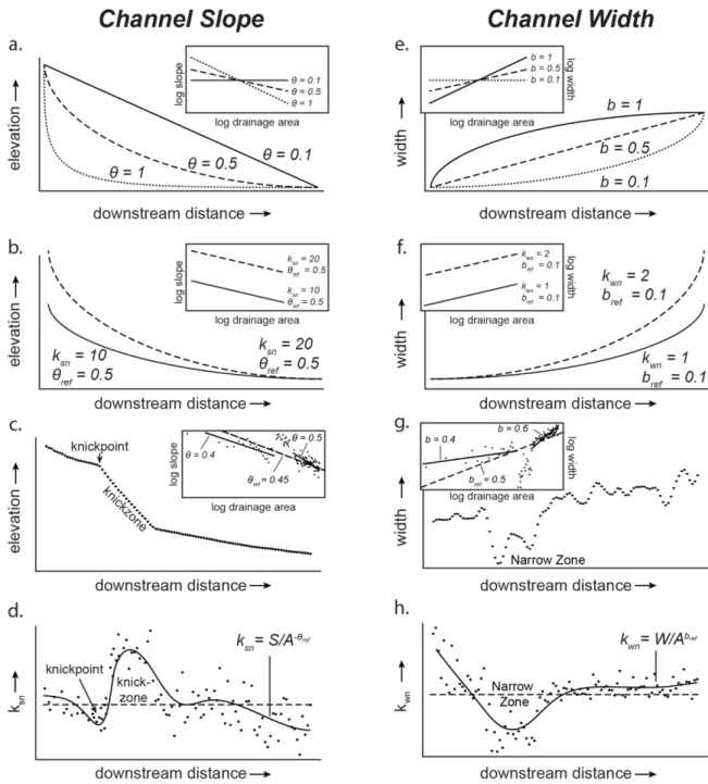
where ks is the steepness index and θ is the concavity index (Figure 1a, b) [Flint, 1974].
The concavity index is determined by fitting a linear regression to slope-area data from
the equilibrium channel reaches (i.e. those without knickpoints, rock uplift rate gradients,
or changes in substrate downstream) (Figure 1c) [Wobus et al., 2006a]. To compare
steepness across channel segments with varying drainage areas and concavity indices, a
regional mean concavity index is determined and used as a reference (θref), allowing for
the empirical calculation of the normalized steepness index,
, (2)
a measure of relative steepness (Figure 1d) [Wobus et al., 2006a]. Normalized steepness
is a useful metric because it can be automatically extracted from digital elevation models
(DEMs) and has been shown to correlate with erosion rate [Kirby and Whipple, 2012].
2.2 Channel Width
Channel width determines the quantity of energy exerted on a channel’s bed per
unit area, with a reduction in width focusing this energy and enhancing incision.
Equilibrium channels exhibit an exponential relationship between width (W) and
6
(3)
where kw is the width coefficient, and b is the width exponent (b ≅ 0.5) (Figure 1e, f)
[Hack, 1957; Montgomery and Gran, 2001; Snyder et al., 2003a]. The width coefficient
can be thought of and used as an empirical parameter of channel geometry, but it can also
be directly related to incision potential based on stream-power models. By combining
incision models under the assumptions of steady-state equilibrium and that slope scales
exponentially with drainage area, the width coefficient, hereinafter referred to as the
wideness index, can be considered the lateral component of channel adjustment related
to incision potential (Appendix A). Similar to θref in equation (2), a mean width exponent
can be determined for equilibrium channel reaches, yielding a reference wideness
exponent (bref) (Figure 1g). Applying bref to width-area data produces the normalized
wideness index,
, (4)
a parameter that allows for quantitative comparison of channel widths across a region
(Figure 1h). We consider downstream variations in kwn to be an empirical measure of the
7
Figure 1. Idealized variations in channel form parameters downstream. Equilibrium long profiles with varying concavity indices (a) and steepness indices (b) with insets displaying slope-area data [modified after Duvall et al., 2004; Whipple and Tucker, 1999]. (c) Long profile with a knickpoint and knickzone. Inset shows reference concavity (slope of dashed line) set by linear regressions through the equilibrium slope-area reaches (gray lines). (d) Long profile of raw (dots) and smoothed (line) normalized steepness index (ksn) from profile in part c. Dashed horizontal line is mean ksn and equivalent to θref (inset of part c).
(e) Equilibrium channel width long profiles with varying width exponents assuming a square increase in drainage area with increasing distance downstream. Inset is the width-area data. (f) Equilibrium long width profiles with varying wideness indices (kwn) and fixed width exponent b. Inset shows same profiles
8
3. GEOLOGIC AND GEOMORPHIC SETTING
Considerable convergence of India with Asia (~20 of ~40 mm/yr) has been
focused near the Himalayan front in the Quaternary [Bilham et al., 1997; England and
Molnar, 1997; Kumar et al., 2001]. Much of this convergence is accommodated along
the Himalayan Frontal Thrust (HFT) [Lavé and Avouac, 2001; Wesnousky et al., 1999].
The HFT is a segmented, blind-to-emergent fault recognized as the main tectonic and
topographic boundary (or discontinuity) between the Himalayas and the Gangetic
foreland (Figure 2) [Kumar et al., 2006; Nakata, 1989]. Shortening along the HFT drives
uplift of foothill ranges that are composed of Tertiary molasse deposits of the Siwalik
Group that hence are called the Siwalik Hills [Malik and Nakata, 2003; Yeats and Lillie,
1991; Yeats and Thakur, 2008]. Bedrock rivers draining the Siwalik Hills are argued to
be in steady-state equilibrium with the active faulting because (1) patterns in river
incision potential match rock uplift rates inferred by dated fluvial terraces [Lavé and
Avouac, 2000, 2001], (2) channels exhibit well-graded elevation profiles where rock
types and uplift do not vary [Kirby and Whipple, 2001], and (3) a combination of weak
uplifting rock and high river discharge during monsoons provide erosionally efficient
river and overland flow that keeps hillslopes near failure by landsliding and allows
channels to rapidly adjust to the active deformation [Barnes et al., 2011].
In northwestern India, the Mohand range is a Siwalik uplift structure that is ~80
by 15 km long with ~500 m of total relief (Figure 2) [Rao et al., 1975]. Geologic and
geophysical data indicate the Mohand is a fault-bend fold in the HFT hanging wall
[Kumar et al., 2006; Powers et al., 1998; Wesnousky et al., 1999]. Here, the HFT has
9
close to the southwestern mountain front near the fold axis (Figure 2b) [Mishra and
Mukhopadhyay, 2002; Powers et al., 1998]. As a consequence of this fault geometry,
average rock uplift rates between the range flanks vary [Barnes et al., 2011], but are
approximately uniform and high across most of the southern flank [Kirby and Whipple,
2012]. However, near the range front, the HFT ramp dip goes to zero resulting in a zone
of little to no rock uplift. Regional magnetostratigraphy data from the Siwaliks rocks
suggest Mohand deformation began <~0.8 Ma [Sangode and Kumar, 2003]. Near the
town of Mohand, a radiocarbon dated uplifted fluvial terrace suggests a HFT slip rate of
≥13.8 ± 3.16 mm/a and a rock uplift rate of 6.9 ± 1.8 mm/a [Wesnousky et al., 1999].
Figure 2. The Mohand range in the Siwalik Hills, northwest India. (a) The topography results from hanging wall uplift above a Himalayan Frontal Thrust (HFT) segment [fault from Raiverman et al., 1990]. (b) Balanced cross section through the central Mohand [simplified from Barnes et al., 2011; Mishra and Mukhopadhyay, 2002]. Blue dashed line is the mean channel elevation. (c) The 10 study area channels flowing southward from the central portion of the range. Channels begin in Upper Siwaliks conglomerates (yellow), cross a transitional contact (dark grey), then traverse Middle Siwaliks sandstones (blue-gray) before entering the foreland. South of the fold axis (dotted line), channels cross a zone devoid of rock uplift above a flat HFT segment within the range front. Contacts from field mapping, fold axis from
10
A linear range front and continuous stratigraphic exposure suggest that the 1st -order geologic structure does not vary along strike within a central portion of the Mohand
(Figure 2). In this study area, bedrock rivers flow southwest from the divide, traversing
down section through Mio-Pleistocene Upper Siwaliks, across a transitional contact, and
then across older Middle Siwaliks before reaching the open foreland (Figure 2c) [Kumar
and Nanda, 1989; Kumar and Ghosh, 1991]. The Upper Siwaliks are thick beds of
quartzite-cobble conglomerates with a sand matrix and the Middle Siwaliks are poorly
indurated multistory sandstones (Figure 3a, c) [Kumar, 1993]. The channels have
bedrock banks and their beds are covered by sand to cobble-sized sediment with
occasional bedrock exposures (Figure 3b, d). Channels occupy most, if not all, of the
valley floor and possess steep cut banks and gentler slopes on the inside of meanders
bends. Bedload size is limited by the cobble-sized clasts sourced from the Upper
Siwaliks conglomerates, the only exception being scattered mass wasting deposits from
the Middle Siwaliks hillslopes. Sediment is predominantly transported down the
channels during the monsoons (80-85% of the mean annual precipitation, ~1-2 m/yr,
occurs July to September [Bookhagen and Burbank, 2006; Mohindra et al., 1992] and
appears to breakdown to a bi-modal size distribution (sand and cobbles) throughout the
channels very quickly (Figure 3). As a result, the channels (a) contain ephemeral rivers
characterized by high discharges implying efficient but episodic sediment transport and
incision [Barnes et al., 2011] and (b) have an average hydraulic roughness that varies
11
Figure 3. Field photos of the Siwaliks stratigraphy and channel-to-hillslope scale geomorphology in the Mohand range. Upper Siwaliks conglomerates contain cobble-sized clasts within a poorly lithified sandstone matrix (a), and channels that are wide with low banks and hillslope relief (b). Middle Siwaliks contain multistory cross-bedded sandstones (c, with person for scale), and channels that are narrow with steep banks and high hillslope relief (d, with person for scale).
4. METHODS
4.1 Field Data
We investigated the Mohand geology and measured proxies for rock erodibility
and channel morphology in selected areas. We augmented existing stratigraphic sections
in the Mohand [Kumar, 1993; Kumar and Nanda, 1989] with our own field observations
of the nature and location of the transition from Upper-to-Middle Siwaliks along 5
12
these locations using the intersection between topography and surfaces projected parallel
to average rock orientation.
Rock erodibility exerts a 1st-order control on river incision and channel morphology [Montgomery and Gran, 2001; Whipple, 2004; Whipple et al., 2000]. Rock
strength and fracture spacing is thought to govern bedrock erodibility [e.g. Hack, 1957;
Selby, 1993; Stock and Montgomery, 1999]. We quantified intact rock strength using a
type N Schmidt Hammer, a spring-loaded device that measures rebound values that scale
with unconfined rock strength estimates made in laboratory tests [Cargill and Shakoor,
1990; Selby, 1993]. We estimated intact rock strength at 10 sites in the Upper Siwaliks
and 13 in the Middle Siwaliks by recording 40 rebound measurements per site and
discarding all measurements below a rebound value of 11 [Duvall et al., 2004; Snyder et
al., 2003a]. In the Upper Siwaliks, we restricted our measurements to the conglomerate
matrix because it is the weakest component and thus sets the bedrock strength limit. We
also estimated intact rock strength with ‘simple means’ field testing [Hack and Huisman,
2002] because the type N Schmidt Hammer is not designed for weak rocks [Goudie,
2006]. This is a semi-quantitative test that classifies a rock’s response to hand
compression and hammer blows. We conducted 20 simple means testing measurements
at each of the same sites. We then compared the mean values of each location and finally
combined them into a single average and standard deviation for the two Siwaliks units.
Bedrock erodibility is also affected by fractures because they increase the
efficiency of hydraulic plucking and promote bedrock weathering by increasing surface
area exposure [Clarke and Burbank, 2011; Hancock et al., 2011]. We measured fracture
13
we used three 1 m scan lines to quantify fracture spacing perpendicular to bedding,
parallel to strike, and parallel to dip [after Dühnforth et al., 2010; Gillespie et al., 1993].
We measured channel form along selected reaches in the field to validate our
remote sensing-based estimates because our method is novel and needed testing. We
measured bankfull width at 40 locations using a handheld laser range finder and
compared these field-based widths to the nearest channel width estimated from the
satellite image. We also measured channel slope with a differential GPS along several
reaches.
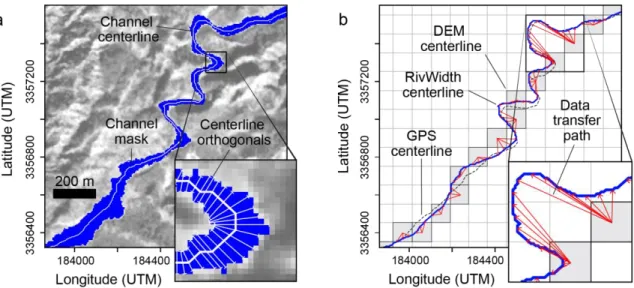
4.2 Remote Sensing
We quantified channel form by combining data extracted from a satellite image
and a DEM. We calculated channel width every ~5-7 m from a SPOT-5 satellite image
(5 m resolution, Bouillon et al. [2006]) with the RivWidth software tool (Figure 4a)
[Pavelsky and Smith, 2008]. We masked channels from their surroundings by the high
contrast between the bright bedload gravels and the adjacent dark vegetation. The
mapped channel width corresponds to peak flow, the effective discharge that sets channel
form, incises, and transports the largest proportion of bedload downstream in bedrock
rivers [Baker, 1977; Lavé and Avouac, 2001; Wolman and Miller, 1960]. We measured
channels from ~1 km beyond the mountain front upstream to where they remained visible
on the satellite image (blue lines in Figure 2c).
We measured channel elevation and upstream drainage area from the 90 m
resolution HydroSHEDS DEM [Lehner et al., 2008] because the 30 m resolution ASTER
GDEM V001 and V002 [Tachikawa et al., 2009] produced major errors in the channel
14
Barnes et al., [2011]) calculated with a modified version of sub-ridgeline relief by
Brocklehurst and Whipple [2002]. Hillslope relief was measured from the ASTER
GDEM V001 because it has a more accurate representation of hillslope gradients than the
90 m DEM [Barnes et al., 2011].
Figure 4. Methods for measuring channel form (location of this example reach in Figure 2c). (a) 5-m resolution SPOT-5 image overlain by RivWidth channel mask (blue) and centerline (white). Inset is channel width (white bars) measured perpendicular to the centerline at each pixel. (b) DEM channel pixels (gray) overlain by channel centerlines determined with RivWidth (blue) and differential-GPS (black) for comparison. Inset shows transfer (red arrows) of DEM-derived information to the image-based channel centerline.
4.3 Data Integration and Calibration of Geomorphic Parameters
We combined the DEM and imaged-based datasets with an algorithm that assigns
data from each channel pixel in the DEM to the nearest image-based channel pixel
(Figure 4b, Appendix B). Real channel gradients are lower than those estimated from the
DEM because the higher resolution image-based channel centerline is longer than the
DEM-derived channel centerline. We correct for this inherent overestimation of channel
15
To reduce noise associated with the data integration process, we smoothed all
parameters downstream using a simple moving average with a window size of 750 m
(Figure B1) [after Duvall et al., 2004]. Thus, we avoid interpretations at streamwise
length scales <750 m. We calculated sinuosity as the ratio of channel length to
straight-line distance between two endpoints spaced 1.5 km along the channel length [e.g.
Mueller, 1968; Stark et al., 2010]. We empirically determined θref = 0.5 in equation (2)
from the slope and drainage area data (Figure B2), and calculated steepness (ksn) at every
pixel downstream. Similarly, we empirically assigned bref = 0.59 in equation (4) from the
width and drainage area data (Figure B3) and calculated wideness (kwn) downstream. To
focus on map-view patterns of channel form, we applied a second smoothing of
steepness, wideness, and shear stress downstream with a 1 km simple moving average
(Figure B1). In map view, we avoid interpretations at streamwise length scales <1.75
km. Finally, when comparing geomorphic parameters between lithologies, we included
all channel reaches upstream from the fold axis so that uniform rock uplift rates could be
assumed.
We modeled incision potential by combining the Manning formula with the
conservation of mass law to obtain the following form of the boundary shear stress
formula,
16
where ρ is the density of water, g is gravity, and n is the Manning friction factor [e.g.
Snyder et al., 2003b; Yanites et al., 2010]. Because measured discharge data is
unavailable for the Mohand rivers, we substituted drainage area for discharge,
(6)
and assumed c = 1, as has been commonly demonstrated [e.g. Hack, 1957; Pazzaglia et
al., 1998] and assumed [e.g. Duvall et al., 2004; Montgomery and Gran, 2001] for
regularly-shaped basins with minimal orographic effects. We eliminated the unknown kq
by dividing the boundary shear stress values by the maximum shear stress value,
eliminating kq and creating a shear stress index, τind that varies from 0 to 1. This index
allows for comparison of relative changes in shear stress rather than absolute values.
5. RESULTS
We analyze changes in lithology, channel geometry, and hillslope relief across the
central Mohand range to account for factors influencing channel form. First, we present
the stratigraphy and associated erodibility of the Upper and Middle Siwaliks. Second, we
validate our remote sensing–based approach and data by comparing the latter with field
measurements. We then show large-scale plan-view patterns of channel form to examine
the spatial distribution of channel adjustment in relation to tectonics and lithology.
Lastly, we examine how variations in channel form and hillslope relief covary
17
5.1 Siwalik Stratigraphy and Erodibility
The Upper-to-Middle Siwaliks boundary is ~0.5 km thick, which translates to a
~1 km wide zone in map view (Figures 2 and 5). This zone contains laterally continuous
meter to decameter thick conglomerate and sandstone interbeds, with the abundance of
conglomerate beds decreasing relative to sandstone beds with increasing distance down
section and downstream. Schmidt Hammer measurements show that the mean intact rock
strength is 47±29% greater in the Middle Siwaliks compared to the Upper Siwaliks
(Figure 5). Testing by simple means shows a similar contrast, with mean intact rock
strength of 16.7±8.4 MPa for the Middle Siwaliks compared to 2.9±3.0 MPa for the
Upper Siwaliks. Within the transitional contact and also the upper portion of the Middle
Siwaliks, intact rock strength gradually increases as the proportion of harder sandstone
beds increases relative to weaker conglomerate beds. Fracture spacing is not
significantly different between the two rock groups (2.9±1.9 fractures/m for the Middle
Siwaliks, 1.8±1.3 for the Upper Siwaliks). We note an ~1 km wide HFT fault zone near
the mountain front where the degree of fracturing increases. These results are consistent
with previous studies that describe both formations as poorly lithified, but the Middle
18
Figure 5. Siwaliks stratigraphy, intact rock strength, and fracture spacing in the Mohand range. Values are means with 1σ errors. (a) Central Mohand stratigraphic column [modified from Kumar, 1993; Kumar and Nanda, 1989]. Note the transitional contact with increasing sandstone abundance down section. (b) Schmidt Hammer rebound values showing a lower mean (vertical dashed lines) intact rock strength value in the Upper Siwaliks compared to the Middle Siwaliks. This indicates the Middle Siwaliks are less erodible. (c) Fracture spacing measurements indicating no difference in mean (vertical dashed lines) spacing between the Upper and Middle Siwaliks within error. Note the increased degree of fracturing near the mountain front associated with the HFT fault zone.
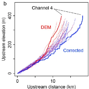
5.2 Remote Sensing Validation
Stretching the DEM-derived elevation data to the channel trace measured from
the satellite image reduces channel slopes (Figure 6a). This process results in more
19
channel gradient reduction occurs in all measured channels and is proportional to the
difference in channel length measured from both data sources (Figure 6b). For example,
highly sinuous channels that contain tight meander bends (e.g. channel 4) produce greater
gradient corrections (Figures 2c and 6c). These corrections influence steepness index,
concavity index, and shear stress and thus should be considered when using any low
resolution DEM to measure channels with tight meander bends.
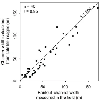
20
Comparison of channel widths measured in the field and from a satellite image
produces a strong 1:1 correlation (Figure 7). On average, there is a small bias for the
remotely-sensed data to underestimate true channel width by ~8% (statistically
significant at 95% confidence interval, p-value = 0.051). Potential sources of deviations
from a 1:1 ratio include channel-masking errors caused by vegetation or hillsides
obscuring the channel bed and registration errors between the two datasets such that
differently located channel width measurements are compared. Regardless, the robust
correlation between the two datasets validates our remote-sensing approach to measuring
channel width continuously downstream.
21
5.3 Channel Form vs. Rock Erodibility
Channel reaches in the weak Upper Siwaliks display a relatively wide range of
mean slopes yet possess a low range in mean channel widths (Figure 8a), while the
inverse is true for the strong Middle Siwaliks. This is in part a function of where each
rock type is located along the channel profiles because slope and width do not necessarily
vary by the same degree with increasing drainage area (e.g. Figure 1 a, e). Thus,
comparing slope and width normalized to drainage area, via steepness (ksn) and wideness
(kwn), produces two more comparable parameters (Figure 8b).
Figure 8. Comparison between channel form and rock erodibility. Values are channel means with 1σ errors, limited to the reaches above the fold axis to eliminate the influence of a change in rock uplift rate on channel form. (a) Channel slope varies more in the Upper Siwaliks whereas width varies more in the Middle Siwaliks. (b) Channels have higher steepness and lower wideness in the Middle Siwaliks than in the Upper Siwaliks. In general, steepness and wideness are inversely correlated. (c) Shear stress index (τind) showing the relative
22
Channels are 32 ± 17% steeper and 70 ± 33% narrower in the Middle Siwaliks than in the
Upper Siwaliks. Similarly, using equation 5, shear stress increases in Middle Siwalik
channels by 68 ± 13% if only channel slope and upstream drainage area are considered,
while shear stress increases by 95 ± 29% when only width and drainage area are
considered (Figure 8c). Together, these results indicate that channels both narrow and
steepen in response to an increase in substrate strength, thereby focusing erosion potential
to erode the stronger uplifting rock.
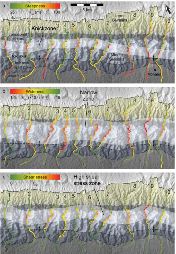
5.4 Channel Form Patterns
Patterns in channel steepness, wideness, and shear stress are systematic across the
study area in plan view. Low steepness in the Upper Siwaliks transitions to an ~2
km-wide zone of high steepness (a knickzone) within the Middle Siwaliks. The position of
this knickzone varies somewhat along strike (Figure 9a). All channels exhibit a narrow
zone ~4 km-wide oriented along strike that begins within or near the transitional contact
and ends ~1-2 km before the range front (Figure 9b). Because shear stress is a function
of channel gradient, width, and upstream drainage area, its variations reflect the
combined changes in steepness and wideness (Figure 9c). All channels display an ~3
km-wide zone of high shear stress beginning within or near the transitional contact.
23
Figure 9. Plan-view patterns of smoothed channel steepness, wideness, and shear stress. (a) Normalized steepness index (ksn) shows a ~2 km-wide knickzone oriented roughly parallel to strike within the Middle
Siwaliks. (b) Normalized wideness index (kwn) shows a ~4 km-wide zone of narrow channels across much
of the Middle Siwaliks north of the fold axis. Downstream of this zone, channels widen, often before reaching the range front. (c) Shear stress index (τind) shows a ~3 km-wide zone of high values, indicative of
24
Variations in channel form also exhibit systematic patterns downstream. First,
channels 1-8 reach a local steepness minimum in or just downstream from the transitional
contact (dashed red line, Figure 10). This steepness minimum is a knickpoint location
and the increase in steepness downstream is a knickzone (e.g. Figure 1c, d). Downstream
past this knickzone, steepness patterns either plateau or slightly increase even beyond the
range front. Second, wideness decreases downstream beginning within or just upstream
from the transitional contact to near the knickpoint (dashed blue line, Figure 10). At the
knickpoint, channels reach a threshold wideness of kwn = ~5 x 10⁻³ m0.59. Then most channels (except channels 1 and 5) remain narrow until near the range front. Third, in or
near the low uplift zone, channels increase their wideness and maintain it into the
foreland plain. This width increase is the main reason for the concomitant decrease in
shear stress across the low uplift zone and into the foreland. Third, in all channels save 1
and 9, sinuosity peaks within or just downstream from the transitional contact (Figure
11). Where sinuosity peaks, all channels except 1 and 3 show minimal wideness (within
25
Figure 10. Downstream variations in channel form along all channels. Locations in Figure 2c. Upstream grey bar is the Upper-to-Middle Siwaliks boundary and the downstream bar is the low uplift zone downstream of the fold axis within the range topography (see Figure 2b, c). Upper panel shows elevation profiles (black) and steepness index (ksn, red). Lower panel shows width profiles (black) and wideness
index (kwn, blue). Shear stress index (τind) is represented by the color gradient between panels. Beginning
26
Hillslope relief and wideness covary inversely with an average correlation of
-0.74±0.25 (r = -0.82±0.07 excluding channel 1). This association holds across both rock
formations and alluvial reaches beyond the mountain front (Figure 11). Conversely,
hillslope relief and steepness show no correlation (r = 0±0.2) when the entire channel
length is considered. However, if only the reaches located upstream from the fold axis
are examined, where uplift rates are approximately uniform, high hillslope relief
corresponds with steep channels in the Middle Siwaliks (Figure 12a). Similarly, strong
lithologies correspond with high hillslope relief and narrow channels (Figure 12b). In
summary, wideness is generally low where steepness, sinuosity, hillslope relief, and rock
27
Figure 11. Downstream variations in sinuosity index (green), wideness index (kwn, blue), and hillslope
28
Figure 12. Comparison between hillslope relief, channel form, and rock erodibility. Values are means with 1σ errors, limited to the channel reaches above the fold axis to eliminate the influence of a change in rock uplift rate on channel form. The erosionally-resistant Middle Siwaliks have higher hillslope relief as well as relatively steeper (a) and narrower (b) channels.
6. DISCUSSION
6.1 Channel Steepness and Wideness Controls
By quantifying channel form both vertically and laterally, we gain a more
complete understanding of the downstream dynamics and mechanisms of channel
adjustment to known changes in rock strength and uplift rate. We observe a knickpoint in
most channels within or near the transitional Siwaliks boundary [see also Kirby and
Whipple, 2012]. Because we infer the rock uplift field to be approximately uniform here,
these knickpoints may reflect either a transient wave of enhanced incision rate [e.g.
Harkins et al., 2007; Whittaker et al., 2007b], or a change in substrate [e.g. Haviv et al.,
2010]. Given the proximity to the change in lithology, we interpret the knickpoints to
reflect the change from the weak Upper Siwaliks to the strong Middle Siwaliks. While it
is possible that the knickpoints are the result of a recent increase in fault slip rate, the
29
Modeling and field studies show that width decreases with increasing slope along
knickzones [Finnegan et al., 2005; Whittaker et al., 2007a; Wobus et al., 2006b].
However, in the Mohand, most channels begin narrowing >1 km upstream of the
knickpoints and reach a minimal wideness at or near them (Figure 10). To explain this
pattern, we hypothesize that as rivers traverse the Siwaliks transition zone where rock
strength increases, their channel banks become better able to resist lateral erosion, thus
decreasing wideness and enhancing incision potential on the bed. Thus rivers initially
maintain a balance between erosivity and rock erodibility by adjusting their shape
laterally rather than vertically. Then, as bedrock erodibility continues to decrease
downstream, channel wideness reaches a minimum threshold of ~5 x 10⁻³ m0.59 (Figure 10), at which point we infer that further narrowing produces less efficient incision due to
energy dissipation on the channel banks [Wobus et al., 2008]. At this point, channels
cease adjusting their width and instead increase their stream power by steepening,
resulting in the formation of a knickzone downstream (Figure 9).
Downstream from the knickzone, most channels remain narrow then dramatically
widen in or near the low uplift zone (Figure 10). Here, channels maintain their steepness
yet increase their wideness to levels comparable to channels in the alluvial foreland. This
wideness increase may reflect (1) an increase in bedrock erodibility induced by brittle
deformation of the HFT [e.g. Kumar et al., 2006], (2) backfilling (i.e. aggradation of
alluvial sediments) due to increased sedimentation near the range front, and/or (3) a
decrease in rock uplift rate. We favor the latter option for several reasons. First,
widening begins near the Mohand fold axis, below which the HFT changes from a
30
~0 mm/yr. Second, we observed more bedrock exposures in the channel beds near the
mountain front, indicating a thin sediment cover, therefore reducing the likelihood of
significant backfilling. Third, although rock fracturing is enhanced near the range front
and reduces rock strength, the HFT fault zone extends only ~1 km into the range front
whereas channel widening begins further upstream.
Shear stress patterns reflect changes in rock strength and uplift rate in steady-state
landscapes where incision is balanced by uplift. In response to an increase in rock
strength downstream, rivers exert more incision capacity through adjustment of their
channel morphologies by widening then steepening. Further downstream, channels
respond to a decrease in rock uplift by increasing their width rather than decreasing their
slope, an observation made elsewhere in similar settings [e.g. Lavé and Avouac, 2001;
Montgomery and Gran, 2001; Yanites et al., 2010]. This change in channel width but not
slope in response to a decrease in rock uplift rate underscores the importance of
considering channel width when estimating incision potential patterns and rates in order
to infer tectonic information where rock erodibility and uplift are not uniform.
6.2 Channel sinuosity controls
Channels not only steepen and narrow to accommodate greater rock strength of
the Middle Siwaliks, they also increase in sinuosity (Figure 11). This is a surprising
observation because increased sinuosity lowers average channel slope, lowering the
vertical incision potential necessary to balance the increased strength of the Middle
Siwaliks. Possible causes for this enhanced meandering include structural control and/or
31
Field observations show that rivers flowing against dip tend to exhibit higher
sinuosity than those flowing downdip [Harden, 1990]. This is because weaker interbeds
promote lateral erosion, causing channels to preferentially align parallel to strike,
whereas stronger beds tend to resist lateral erosion, directing the channel across strike.
While all studied rivers in the Mohand flow across dip, reaches in the upper Middle
Siwaliks traverse through sandstone and conglomerate interbeds with highly variable
strength (Figure 5). This may explain the peak in sinuosity occurring in most channels
within or near the transitional contact (Figure 11). This suggests that small-scale
variations in sedimentary layering can significantly impact average channel form and be
observed by combining field and remote sensing based measurements.
Another potential mechanism for enhanced sinuosity in the Middle Siwaliks is the
role channel sediment plays in controlling vertical and lateral erosion. At low flows,
sediment protects the underlying bedrock, but when flow increases to a critical shear
stress, sediment is entrained as bedload and acts as tools that enhance bedrock erosion
[Gilbert, 1877; Lague et al., 2005]. In Mohand, a thick sediment layer almost entirely
covers the channel beds whereas the banks are primarily bare bedrock (Figure 3). During
lower magnitude/higher frequency flows, only the uppermost bedload is mobilized,
thereby eroding the channel banks but not incising into the rock below the bed [Finnegan
et al., 2007; Turowski et al., 2008; Yanites et al., 2011]. This process requires an
adequate supply of coarse sediment to the channel for a given discharge such that the bed
is protected except during high magnitude discharges [Moore, 1926; Snyder et al.,
2003b]. Such is the case in the Mohand, where the Upper Siwaliks conglomerate
32
This process of increased lateral erosion during lower flows can lead to an
increase in sinuosity or widening depending on the ratio of river erosivity to bedrock
strength. In the strong Middle Siwaliks, the ratio is relatively low, producing banks that
resist lateral erosion, confine rivers to narrow channels, and generally influence the
plan-view path of the river. During moderate flows, helicoidal currents preferentially erode
cut banks causing channels to migrate laterally [Shepherd, 1972]. During higher
discharge events, sediment is mobilized and vertical incision occurs more evenly across
the bed [Shepherd, 1972], thereby carving the channel deeper into the sinuous path
established by the lower flows. In contrast, we suggest that in the weaker Upper
Siwaliks, the ratio of river erosivity to rock erodibility is high resulting in channel banks
that are unable to “steer” the river’s course. Thus, channels flowing through weak rocks
with ample sediment supply tend to widen rather than meander.
6.3 Channel Wideness and Hillslope Relief
Channel wideness and hillslope relief in the Mohand show a strong inverse
correlation (r = -0.74±0.25) suggesting that (1) channel width and hillslope relief are
shaped by common forces and/or (2) a connection exists between bedrock channel
dynamics and hillslope processes. Channel width and hillslope relief share common
sources of influence such as lithology, rock uplift rate, and climate [e.g. Schmidt and
Montgomery, 1995]. Climate does not vary much across the study area, thus rock
erodibility and uplift rate are the main factors applicable to both. Given the diverse
influences of channel width (e.g. bedload sediment supply and grain size, runoff
33
hillslope relief (e.g. valley spacing, soil production, vegetation type and density [Gabet et
al., 2004 and references therein]), it is surprising that such a strong correlation exists.
A possible cause for this strong correlation is a connection between bedrock
channel dynamics and hillslope processes. The stronger Middle Siwaliks facilitate high
hillslope relief and channel banks, producing larger, deeper-seated mass wasting events
on the hillslopes near the channel banks. Thus, more debris is delivered to channels in
larger magnitude, lower frequency, contributions such that the channels flowing through
Middle Siwaliks may be influenced differently than the Upper Siwaliks. At the location
of cut bank failures in the Middle Siwaliks, channels are diverted around the foot of the
landslide deposit, increasing sinuosity, creating a knickpoint, and narrowing channel
width [Gillespie et al., 1993; Gran and Montgomery, 2005 2012]. This apparent link of
fluvial and hillslope processes may explain the highly scattered relationship between
channel width and drainage area in bedrock rivers [e.g. Montgomery and Gran, 2001;
Wohl and David, 2008]. Because hillslope relief can be automatically calculated from
DEMs, this relationship could be used to estimate relative variations in channel width
directly from a DEM. Further study is needed to determine if hillslope relief and
normalized wideness index scale in other settings.
7. SUMMARY AND CONCLUSIONS
Channel form reflects changes in rock strength and uplift rate in the Mohand, if
both width and slope are explicitly considered. We hypothesized that channel width may
adjust independently of drainage area and/or slope in response to spatial variations in
34
the northwest Himalaya using a new method that integrates continuous measurements of
fluvial parameters (channel width, slope, sinuosity, adjacent hillslope relief) from remote
sensing data. We observed that channels are 32 ± 17% steeper and 70 ± 33% narrower in
the erosionally resistant Middle Siwaliks compared to the weaker Upper Siwaliks.
Further, channels begin to narrow to a minimum wideness of ~5 x 10⁻³ m0.59 over a kilometer upstream from where they steepen in response to a gradational increase in rock
strength associated with a transitional stratigraphic boundary. In response to a decrease
in rock uplift rate at the mountain front, channels increase their wideness rather than
adjust their steepness. We also observed that rivers flowing across alternating strong and
weak beds exhibit increased sinuosity, suggesting that fine-scale variability in bedrock
strength via sedimentary interbedding can influence average steepness values. Finally,
normalized wideness index scales linearly with hillslope relief in the Mohand range,
hinting at a potentially useful proxy for estimating channel width from DEMs. This
study highlights the importance of rock strength in influencing channel form and
promotes the inclusion of channel width measurements when trying to extract tectonic
35
APPENDIX A
WIDENESS INDEX DERIVATION
The wideness index can be used as an empirical measure of deviation from an
equilibrium width-area scaling, but it can also be related to incisional potential. The
derivation of the wideness index closely follows that of the steepness index [see appendix
in Duvall et al., 2004; Whipple and Tucker, 1999]. However, rather than assuming
channel width scales with drainage area, we rely on the relationship that channel slope
exhibits an equilibrium scaling with drainage area as described in equation 1. The
wideness index is derived from the stream-power family of models that equate bedrock
incision rate (E) to a power function of boundary shear stress (τb) which must exceed a
threshold of critical shear stress (τc),
[ ] , (A1)
where ke depends on rock erodibility, f(qs) describes the dual role entrained sediment
plays as both tools or cover for incision, and ae depends on the erosion mechanics
[Howard and Kerby, 1983; Whipple et al., 2000]. We assume that the influence of
critical shear stress (τc) and entrained sediment (f(qs)) are negligible because (a) the
effective discharge that shapes bedrock channels typically far exceeds this value in the
Siwalik Hills [Kirby and Whipple, 2012], and (b) sediment flux scales with shear stress
[Bagnold, 1980].
Incision rate is reduced to terms of boundary shear stress, which under
36
, (A2)
where kt, α, and β are constants that depend on flow resistance dynamics [e.g. Yanites et
al., 2010]. Combining (1, 3, 6, A1, and A2) yields,
, (A3a)
where
, (A3b)
, (A3c)
. (A3d)
(A3a) resembles the form of the generalized total stream-power model [Howard and
Kerby, 1983], except in terms of lateral channel parameters rather than slope.
If steady-state equilibrium conditions exist, such that long term rock uplift rate
(U) and bedrock incision rate are balanced and the channel bed elevation does not vary
with time ( ), then
37
which can be rearranged to solve for equilibrium channel width,
. (A5)
This takes the form similar to the width-area formula of (3),
, (A6a)
where kw is the wideness index, and b is the width exponent with the implied relations,
(9b)
. (9c)
The width exponent can be empirically determined by plotting channel width and
drainage area in log-log space and taking linear regressions of channel reaches that
38
APPENDIX B
DATA INTEGRATION AND SMOOTHING
We developed an algorithm in R code [Pebesma et al., 2012] that integrates,
analyzes, and displays channel morphometric data. The algorithm combines topographic
information (elevation, upstream drainage area, and hillslope relief) with plan-view
channel information (channel width, length, and sinuosity) by assigning data from the
nearest DEM pixel to each pixel along the image-based channel centerline (Figure 4b).
To reduce error, the algorithm matches data only within the same channel and at, or
downstream of, the previous DEM pixel sampled. Because of spatial variability among
datasets, DEM pixels are sampled unevenly in the integration processes resulting in a
stair stepped pattern on the elevation profiles in the image-corrected dataset (Figure 6b).
This stair-step effect, combined with occasional misalignment of tributary junctions
between the DEM and image, requires some smoothing of all morphometric variables to
reduce noise.
We initially smoothed channel elevation, width, upstream drainage area and
hillslope relief data using a downstream simple moving average with a window size of
750 m (Figure B1a, b, d, e, f) [after Duvall et al., 2004]. We then determined the
reference concavity index and width exponent by taking the average slope of linear
regressions fit to all equilibrium channel reaches (Figure B2, B3) and calculated
steepness and wideness indices at every pixel using θref = 0.5 and bref = 0.59. Figure 9
shows smoothed normalized steepness, wideness, and shear stress indices using a simple
moving average with a window size of 1 km downstream distance, a length necessary to
39
Figure 13. Example channel (2 in Figure 2c) showing raw (gray) and smoothed (black) data. Elevation (a), upstream drainage area (b, f), hillslope relief (d), and width (e), were smoothed with a 750 m simple moving average (Figure 10, 11) [after Duvall et al., 2004]. Steepness (ksn) (c), wideness (kwn), and shear
stress (τind) (h) indices with a 1 km simple moving average, a window length necessary for the display of
40
41
42
REFERENCES
Amos, C. B., and D. W. Burbank (2007), Channel width response to differential uplift, J. Geophys. Res., 112(F2), F02010, doi: 10.1029/2006jf000672.
Anderson, R. S. (1994), Evolution of the Santa Cruz Mountains, California, through tectonic growth and geomorphic decay, J. Geophys. Res., 99(B10), 20161-20179, doi: 10.1029/94jb00713.
Bagnold, R. A. (1980), An Empirical Correlation of Bedload Transport Rates in Flumes and Natural Rivers, Proceedings of the Royal Society of London. A. Mathematical and Physical Sciences, 372(1751), 453-473, doi: 10.1098/rspa.1980.0122.
Baker, V. R. (1977), Stream-channel response to floods, with examples from central Texas, Geol. Soc. Am. Bull., 88(8), 1057-1071, doi:
10.1130/0016-7606(1977)88<1057:srtfwe>2.0.co;2.
Barnes, J. B., A. L. Densmore, M. Mukul, R. Sinha, V. Jain, and S. K. Tandon (2011), Interplay between faulting and base level in the development of Himalayan frontal fold topography, J. Geophys. Res., 116(F3), F03012, doi:
10.1029/2010jf001841.
Bilham, R., K. Larson, and J. Freymueller (1997), GPS measurements of present-day convergence across the Nepal Himalaya, Nature, 386(6620), 61-64, doi: 10.1038/386061a0.
Bookhagen, B., and D. W. Burbank (2006), Topography, relief, and TRMM-derived rainfall variations along the Himalaya, Geophy. Res. Lett., 33(8), L08405, doi: 10.1029/2006gl026037.
Bouillon, A., M. Bernard, P. Gigord, A. Orsoni, V. Rudowski, and A. Baudoin (2006), SPOT 5 HRS geometric performances: Using block adjustment as a key issue to improve quality of DEM generation, ISPRS J. Photogram. Rem. Sens., 60(3), 134-146, doi: 10.1016/j.isprsjprs.2006.03.002.
Brocklehurst, S. H., and K. X. Whipple (2002), Glacial erosion and relief production in the Eastern Sierra Nevada, California, Geomorphology, 42(1–2), 1-24, doi: 10.1016/s0169-555x(01)00069-1.
Burbank, D., J. Leland, E. Fielding, R. Anderson, N. Brozovic, M. Reid, and C. Duncan (1996), Bedrock incision, rock uplift and threshold hillslopes in the northwestern Himalayas, Nature, 379(6565), 505-510, doi: 10.1038/379505a0.
43
Clarke, B. A., and D. W. Burbank (2011), Quantifying bedrock-fracture patterns within the shallow subsurface: Implications for rock mass strength, bedrock landslides, and erodibility, J. Geophys. Res., 116(F4), F04009, doi: 10.1029/2011jf001987.
Dühnforth, M., R. S. Anderson, D. Ward, and G. M. Stock (2010), Bedrock fracture control of glacial erosion processes and rates, Geology, 38(5), 423-426, doi: 10.1130/g30576.1.
Duvall, A., E. Kirby, and D. Burbank (2004), Tectonic and lithologic controls on bedrock channel profiles and processes in coastal California, J. Geophys. Res., 109(F3), F03002, doi: 10.1029/2003jf000086.
England, P., and P. Molnar (1997), Active Deformation of Asia: From Kinematics to Dynamics, Science, 278(5338), 647-650, doi: 10.1126/science.278.5338.647.
Finnegan, N. J., L. S. Sklar, and T. K. Fuller (2007), Interplay of sediment supply, river incision, and channel morphology revealed by the transient evolution of an experimental bedrock channel, J. Geophys. Res., 112(F3), F03S11, doi: 10.1029/2006jf000569.
Finnegan, N. J., G. Roe, D. R. Montgomery, and B. Hallet (2005), Controls on the channel width of rivers: Implications for modeling fluvial incision of bedrock,
Geology, 33(3), 229-232, doi: 10.1130/g21171.1.
Flint, J. J. (1974), Stream gradient as a function of order, magnitude, and discharge,
Water Resour. Res., 10(5), 969-973, doi: 10.1029/WR010i005p00969.
Gabet, E. J., B. A. Pratt-Sitaula, and D. W. Burbank (2004), Climatic controls on hillslope angle and relief in the Himalayas, Geology, 32(7), 629-632, doi: 10.1130/g20641.1.
Gilbert, G. K. (1877), Geology of the Henry Mountains (Utah), U.S. Geog. Geol. Surv. Rocky Mt. reg., 160.
Gillespie, P. A., C. B. Howard, J. J. Walsh, and J. Watterson (1993), Measurement and characterisation of spatial distributions of fractures, Tectonophysics, 226(1-4), 113-141, doi: 10.1016/0040-1951(93)90114-Y.
Goode, J. R., and E. Wohl (2010), Substrate controls on the longitudinal profile of bedrock channels: Implications for reach-scale roughness, J. Geophys. Res.,
115(F3), F03018, doi: 10.1029/2008jf001188.
Goudie, A. S. (2006), The Schmidt Hammer in geomorphological research, Prog. Phys. Geog., 30(6), 703-718, doi: 10.1177/0309133306071954.
44
loading at Mount Pinatubo, Philippines, Geol. Soc. Am. Bull., 117(1-2), 195-211, doi: 10.1130/b25528.1.
Hack, J. T. (1957), Studies of longitudinal stream profiles in Virginia and Maryland, US Geol. Surv. Prof. Pap., 45-97.
Hack, R., and M. Huisman (2002), Estimating the intact rock strength of a rock mass by simple means, in 9th Congr.of the Int. Ass. Engin. Geol. Env., edited by J. L. van Rooy and C. A. Jermy, Engineering Geology for Developing Countries, Durban, South Africa.
Hancock, G. S., E. E. Small, and C. Wobus (2011), Modeling the effects of weathering on bedrock-floored channel geometry, J. Geophys. Res., 116(F3), F03018, doi: 10.1029/2010jf001908.
Harbor, D. J. (1998), Dynamic Equilibrium between an Active Uplift and the Sevier River, Utah, J. Geol., 106(2), 181-194, doi: 10.1086/516015.
Harden, D. R. (1990), Controlling factors in the distribution and development of incised meanders in the central Colorado Plateau, Geol. Soc. Am. Bull., 102(2), 233-242, doi: 10.1130/0016-7606(1990)102<0233:CFITDA>2.3.CO;2.
Harkins, N., E. Kirby, A. Heimsath, R. Robinson, and U. Reiser (2007), Transient fluvial incision in the headwaters of the Yellow River, northeastern Tibet, China, J. Geophys. Res., 112(F3), F03S04, doi: 10.1029/2006jf000570.
Haviv, I., Y. Enzel, K. X. Whipple, E. Zilberman, A. Matmon, J. Stone, and K. L. Fifield (2010), Evolution of vertical knickpoints (waterfalls) with resistant caprock: Insights from numerical modeling, J. Geophys. Res., 115(F3), F03028, doi: 10.1029/2008jf001187.
Howard, A. D. (1994), A detachment-limited model of drainage basin evolution, Water Resour. Res., 30(7), 2261-2285, doi: 10.1029/94wr00757.
Howard, A. D., and G. Kerby (1983), Channel changes in badlands, Geol. Soc. Am. Bull.,
94(6), 739-752, doi: 10.1130/0016-7606(1983)94<739:CCIB>2.0.CO;2.
Kirby, E., and K. Whipple (2001), Quantifying differential rock-uplift rates via stream profile analysis, Geology, 29(5), 415-418, doi:
10.1130/0091-7613(2001)029<0415:qdrurv>2.0.co;2.
Kirby, E., and K. X. Whipple (2012), Expression of active tectonics in erosional landscapes, J. Struct. Geol., doi: 10.1016/j.jsg.2012.07.009.
![Figure 2. The Mohand range in the Siwalik Hills, northwest India. (a) The topography results from hanging wall uplift above a Himalayan Frontal Thrust (HFT) segment [fault from Raiverman et al., 1990]](https://thumb-us.123doks.com/thumbv2/123dok_us/8214578.2177838/18.918.138.784.505.851/figure-siwalik-northwest-topography-himalayan-frontal-segment-raiverman.webp)