How to Construct Fundamental Risk Factors?*
M. Lambert1 G. Hübner2
* The authors would like to thank Marti Gruber, Antonio Cosma, Michel Robe, and Dan Galai for helpful comments.
Georges Hübner thanks Deloitte (Luxembourg) for financial support. The present project is supported by the National Research Fund, Luxembourg.
1 Corresponding Author. Presenter. Researcher, Luxembourg School of Finance, and Ph.D Candidate, HEC
Management School - University of Liège and University of Luxembourg. Mailing address: marie.lambert@uni.lu, Luxembourg School of Finance, rue Albert Borschette, 4, L-1246 Luxembourg (Luxembourg). Phone: (+352)4666446805. Fax: (+352) 352 46 66 44 6835
2 HEC Management School, University of Liège, Belgium Faculty of Economics and Business Administration,
Maastricht University, the Netherlands; Gambit Financial Solutions, Belgium. Mailing address: G.Hubner@ulg.ac.be, HEC Management School - University of Liège, rue Louvrex, 14, B 4000 Liège (Belgium). Phone: (+32) 42327428.
Abstract
Our paper reexamines the methodology of Fama and French (1993) for creating US empirical risk factors, and proposes an extension on the way to compute the mimicking portfolios. Our objective is to develop a modified Fama and French methodology that could be easily implemented on other markets or that could also easily price other risk fundamentals. We raise three main problems in the F&F methodology. First, their annual rebalancing is consumptive in long time-series which sometimes simply do not exist for small exchange markets. Moreover, this does not match with the investment horizon of the investors. Second, their independent sorting procedure underlying the formation of the 6
F&F two-dimensional portfolios causes moderate level of correlation between premiums. Finally,
sorting the stocks into portfolios according to NYSE stock returns tend to over-represent the proportion of small stocks in small and value portfolios. We estimate, along our technology, alternative premiums for the size, book-to-market and momentum risk fundamentals. We compare these three risk premiums to the Fama and French and Carhart benchmarks that Kenneth French make available on his website. In an analysis framework without data snooping bias, we show evidence that although they are correlated, the original F&F premiums and our versions of the F&F premiums bring complementary information. Furthermore, we find that our empirical model better complements the market model for explaining cross-sectional dispersion in returns than the F&F premiums.
Keywords: Fama and French Factors, Momentum, Hedge/mimicking Portfolios, Market Risk Fundamentals
Jel code: G11, G12
How to Construct Fundamental Risk Factors?
A large variety of multifactor models of security returns coexist in the financial literature. Connor (1995) classifies them into three types: macroeconomic, statistical, and fundamental. In macroeconomic models, each security’s rate of return is assumed to be linearly related to the movements of observable economic time-series like the market return, the excess return to long-term government bond, or commodities1. The statistical modeling of security returns relies on factor analysis (principal component analysis, clustering,… )2. Finally, fundamental factor models use market fundamentals like market capitalization, book-to-market, or the levels of skewness and excess kurtosis of stock returns as factor betas3. According to Connor (1995), this latter approach has outperformed the previous ones for the traditional assets. The four-factor Carhart model is indeed largely used in the literature for modeling stock returns.
The challenge in fundamental models is to constitute mimicking or hedge portfolios able to capture the marginal returns associated with a unit of exposure to each attribute4. To achieve this objective, one can perform a Fama and MacBeth (1973) type of regression on the risk fundamentals in order to extract unit-beta portfolios. One can also construct portfolios by aggregating assets according to their correlations with the fundamentals (see Balduzzi and Robotti, 2005). Nonetheless, over time, the mimicking portfolios for size and book-to-market risks developed by Fama and French (1993) have become a standard in constructing fundamental risk factors. These authors consider two ways of scaling US stocks, i.e. a sort on market equity and a sort on book-to-market, and construct six value-weigthed two-dimensional portfolios at the intersections of the rankings. The size factor measures the return differential between the average small cap and the average big cap portfolios, while the
book-to-market factor measures the return differential between the average value and the average growth
portfolios. Both sets of portfolios are rebalanced on a yearly basis. Carhart (1997) completes their three-factor model by computing, along a similar method, a momentum factor that reflects the return differential between the highest and the lowest prior-return portfolios.
1 Among the most referenced studies, we find the market model of Sharpe (1964), Lintner (1965) and Mossin (1966),
the Sharpe style analysis (1992) for mutual funds and its extension for Hedge Funds (Agarwal and Naik,2000)
2 Several applications have been proposed in the field of hedge funds. In particular, we refer to the analyses of Fung
and Hsieh (1997), Brown and Goetzmann (2004) and Gibson and Gyger (2007).
3 See a.o. the models of Fama and French (1993) and Carhart (1997) for the traditional investment analysis, the
analysis of Moreno and Rodriguez (2009) for mutual funds, and finally the models of Kat and Miffre (2006) and Agarwal et al. (2008) for Hedge Funds.
4 Huberman, Kandel and Stambaugh (1987) discuss some criteria that mimicking portfolios must comply with in order
to serve in place of factors in an asset-pricing model. They show that unit-beta portfolio can be used as explanative factor.
The Fama and French (F&F) methodology is however ad hoc with regard to the US stock market. For instance, they only use the NYSE stocks to define the sorting breakpoints in order not to be tilted towards the numerous small stocks of the Nasdaq and Amex exchanges. Likewise, the F&F methodology is also rather arbitrary regarding the way risk fundamentals are priced. They perform two-sorts for size and three-sorts for book-to-market on the heuristic basis that size is less informative than book-to-market. Besides, the yearly rebalancing of their portfolios does not match the investment horizon of investors.
Carhart (1997) was the first author to raise what could be seen as a criticism to the Fama and French approach. To construct his momentum factor, he redefines the 2x3 sorts and the yearly rebalancing of F&F into a 3x3 sorts and a rebalancing on a monthly basis. A recent study of Cremers et al. (2008) also expresses direct criticisms about the F&F method. They show that F&F do not consistently price passive index factors and do not even consistently price portfolios sorted on size and book-to-market. They propose some alternative guidelines for creating the factors and conclude to a superiority of their set of premiums.
Moreover, to be applicable on other markets or other risk fundamentals, the F&F methodology needs to be extended or generalized. Some contributions have already been made in this direction. Faff (2001) develops new proxies for the F&F factors for small exchange markets like the Australian one. He uses style index data rather than constructing the 6 size and book-to-market sorted-portfolios. The estimated size factor is however inconsistent with F&F results as it displays a negative average return over the period. The F&F methodology has also been adapted for factoring non-traded characteristics into returns. For example, Easley et al. (2005) use the F&F method to factor the use of private information into returns.
Besides, Ajili (2005), Kat and Miffre (2006), Kole and Verbeek (2006), and recently Agarwal
et al. (2008) and Moreno and Rodriguez (2009) use the F&F methodology to construct coskewness
and/or cokurtosis mimicking portfolios. All these technologies lead to premiums whose descriptive statistics are inconsistent with the literature, indicating that the method should be improved.5
We view our contribution as methodological. We revisit the procedure introduced by Fama and French for creating risk factors, and propose an alternative way of computing the mimicking portfolios
5 The cokurtosis factor of Kole and Verbeek (2006) displays a negative average return (June 1974 - November 2003)
although positive excess in cokurtosis has been shown to be rewarded in equity market. The skewness premium of Kat and Miffre (2006) is negative over the period (1985-2004) although investors should earn compensation for exposure to negative systematic skewness. Finally, the volatility and the kurtosis premiums of Agarwal et al. (2008) are also
for the same size, value and momentum dimensions6. Our objective is to develop a modified Fama and French procedure that could be easily implemented on other markets or price other risk fundamentals. In order to test our methodology, we estimate the size, book-to-market and momentum risk factors and compare these three risk premiums to the publicly available Fama and French and Carhart benchmarks (referred hereafter as the F&F factors), which are commonly used in empirical studies7. We conduct our analysis on a sample of monthly data downloaded from Thomson Financial DatastreamInc8. We perform our analysis on a recent period of time: the actual sample for the risk premiums range from May 1980 to April 2007, i.e. a total of 324 monthly observations.
We first find evidence of the complementary character of the F&F size, book-to-market and the Carhart momentum factors and of our alternative specification of these premiums. Each set of premiums adds explanatory power to the other one. Moreover, our specification of the empirical risk premiums adds more explanatory power to the market model than the original F&F and Carhart premiums do. Both models deliver equivalent levels of pricing errors. The F&F model tends to underestimate risk, while our alternative model overestimates it. We also test each model specification against the other one. The modified F&F premiums appear to deliver slightly superior results to the original empirical risk premiums. Therefore, if we have to choose one or the other specification, all evidence indicates that our model should be preferred.
The rest of the paper is structured as follows. Section I starts with reviewing the Fama and French methodology. It addresses the issues surrounding their approach, and develops the modifications we bring to F&F premiums construction. Section II describes the data used in this paper, i.e the sample including the dependent and the independent datasets. Section III tests the complementary character of each set of premiums through nested models. Section IV tests the superiority between the two sets of premiums through non-nested models. Section V concludes.
6 Empirical risk factors have long been known to have interesting return patterns. We acknowledge the debate about
the nature of these risk factors. According to Fama and French (1993), they are proxy for nondiversifiable risks, while for Daniel and Titman (1997), it is the characteristics rather than the covariance structure that are priced in these mimicking portfolios. This debate is however not the purpose of our research as the interest of the paper does not reside in the 3 empirical factors but in the new technology for creating risk factors.
7 http://mba.tuck.dartmouth.edu/pages/faculty/ken.french/data_library.html
8 As our purpose is to define guidelines for constructing benchmarks of risk that would be valid for any database, the
I. Review of the Fama and French Methodology
In the Fama and French framework, stocks are not only priced according to their sensitivity to the market portfolio, but also for their co-variations with two hedge portfolios that reflect the return differential between small and big capitalizations, and between value and growth stocks. Carhart (1997) completes the Fama and French model by computing, along a similar method, a momentum factor. It captures the difference in returns between the highest and the lowest prior-return portfolios. In this section, we review how Fama and French compute these risk premiums. We address the issues surrounding their methodology when one wants to extend it to other market or to other risk fundamentals. Next, we describe the modifications brought to the F&F method.
I.1 Issues surrounding the portfolio construction methods
Fama and French (1992) consider two ways of scaling stocks: a sort on market equity, and a sort on book-to-market. They perform two independent sorts onto a full cross-section of US stocks returns (for which book-to-market9 and market equity10 values are available). On his website, Kenneth French completes the F&F framework by performing an additional sort on momentum. Six portfolios are formed on size (ME) and book-to-market (BE/ME), and another six on size and prior (lagged 2 to 12 months) return. Stocks are scaled11 according to one breakpoint for size and two for BE/ME and momentum series, because Fama and French (1993) consider that size is less informative for the cross-sectional variations of stocks than the two other variables.
Value-weighted portfolios are then formed by intersecting the rankings. Size-BTM portfolios are rebalanced every June of year y according to the market equity of December of y-1 and according to the book equity for fiscal year ending in calendar in year y-112. Size and MOM portfolios are rebalanced every month according to the prior 2-12 months return and the market equity for t-1. To feature in the momentum portfolios for month t (formed at the end of t-1), a stock must have a ME for t-1, and a market price at the end of month t-13.
The empirical factors are defined on the basis of these six value-weighted portfolios. First, the
size factor (SMB) is the equally-weighted average return on the three small portfolios minus the
9 Book-to-market is defined as the ratio of the firm’s book value of common equity, BE, to its market value, ME. 10 Size is defined as market equity, ME, i.e. stock price times shares outstanding.
11 Temporary disappearances, missing values, or unrealistic values in any firm time-series simply exclude the related
stocks from the analysis for that time.
12 To be included in the portfolio for month
t (from July of year y to May of year y+1), each share must have an
average return on the three big portfolios. Second, the BTM factor (HML) is the equally-weighted average return on the two value portfolios minus the average return on the two growth portfolios. Finally, the momentum factor is the average return on the two high prior-return portfolios minus the average return on the two low prior-return portfolios. The breakpoints used to allocate stocks into different portfolios are respectively the median NYSE market equity for size, and the 30th and 70th NYSE percentiles for the two other dimensions. F&F use NYSE breakpoints to avoid a skewed distribution of market fundamentals towards bigger market capitalizations. They view the extremely small market values on Amex and NASDAQ as potential biases for the breakdown of the risk space.
Direct and indirect criticisms about the F&F method can be found in the literature. Among the critics of the Fama and French work, Carhart (1997) raises two issues: the 2x3 sorts and the yearly rebalancing. Moreover, the recent study of Cremers et al. (2008) also addresses a direct issue of the Fama and French method. According to them, the Fama and French technology places too much weight on small cap value stocks when averaging the 2x3 sorted portfolios into the factor returns. Our extension of the definition of the sorting breakpoints to all US stocks rather than only the NYSE stocks is motivated by a similar concern. We do not think that the equally-weighted average of the 2x3 portfolios could bias the factor as the set of 2x3 portfolios are value-weighted. However, by limiting the definition of the sorting breakpoints to the NYSE stocks, the F&F method leads to consider bigger portfolios of small caps, with two unfortunate effects. On the one hand, this leads to diversifying the risk related to small stocks as it mixes small and mid caps. On the other hand, it tends to overestimate
the value premium as the value effect is more important in small caps than in big caps (Griffin et al.,
2002; Cremers et al., 2008). Besides, Cremers et al. (2008) considers small and big caps separately when pricing the value factor. Finally, as market indices are often defined along four dimensions for size and only along two for value effects, Cremers et al. (2008) consider the impact on their premiums specification to follow this breakdown. We consider that this point in their technology is equally arbitrary as some of the F&F choices.
Indirect criticisms concern works that do not attempt to modify the Fama and French method for creating US empirical SMB and HML – like in this paper – but rather want to generalize it either on other exchange markets or on other risk fundamentals.
According to Faff (2001), the F&F methodology is not easily transposable in other markets. Through their annual rebalancing, they are consumptive in reliable data over quite long period (more than one year of data is required for each premium time value) that sometimes do not exist. The F&F methodology can sometimes not be simply extended to other sources of risk either. For instance, when constructing moment-related factors, correlations between odd and even moment are so negative that a
simple intersection of independent ranking could lead to empty or severely unbalanced portfolios. On the one hand, as a way to overcome this issue, Ajili (2005), Kole and Verbeek (2006), and Moreno and Rodriguez (2009) construct one-dimensional portfolios for mimicking coskewness and cokurtosis factors, but this approach causes strong correlations between the premiums and could lead to inconsistent situation where the average value of the premium is negative. On the other hand, Agarwal et al. (2008) perform a conditional sorting procedure.
From this discussion, the extensions provided to the Fama and French technology seem to be quite heterogeneous. There appears to be no consensus about how to best construct risk premiums.
I.2 The modified F&F portfolio construction method
Our approach differs from the F&F methodology on various points. First, we consider a comprehensive approach of three dimensions of risks. Second, we propose a consistent and systematic sorting of all listed stocks whereas F&F perform a heuristic split according to NYSE stocks. Third, our monthly rebalancing13 of the portfolios captures more realistically the returns that a financial agent can expect from her exposure to different risks. Fourth and finally, our sequential sorting technique avoids spurious significance in risk factors related to any correlation between the rankings underlying the construction of the benchmarks.
We consider the cross-section of US stock returns and model this risk space as a cube. We split the sample according to three levels of size, BTM, and momentum. Two breakpoints (1/3th and 2/3th percentiles) are used for all fundamentals. Thus, not 6 but 27 portfolios are formed. The breakpoints are based on all US market, not only on NYSE stocks. Figure 1 illustrates this cubic risk approach.
< Insert Figure 1 here >
Our objective is to detect whether, when it is made conditional on two of the three risk dimensions, there is still variation related to the third risk criterion. Therefore, we substitute F&F’s “independent sort” with a “sequential or conditional sort”, i.e. a multi-stage sorting procedure. Namely, we perform successively three sorts. The first two sorts are operated on “control risk” dimensions, while we end with the risk dimension to be priced. The sequential sorting produces 27 portfolios capturing the return related to a low, medium, or high level on the risk factor, conditional on the levels registered on the two control risk dimensions. Taking the difference between the portfolios scoring
high and low on the risk dimension to be priced, but scoring at the same level for the two control risk dimensions, we obtain the return variation related to our risk under consideration.
In such a sequential setting, the premiums capture the return attached to one risk dimension, after having controlled for the two other risk dimensions. An independent sorting like in Fama and French (1993) would be contaminated by the correlations across the risk dimensions, and so across the rankings. Of course, introducing the three F&F empirical risk premiums in a multiple regression would let the risk exposures fight it out and would control for these cross-correlations between premiums. Our objective is however somewhat different as we want to deliver premiums that can be used on their own and that do not require that all three empirical risk premiums are included in the same regression. To achieve this goal, the control for the other two sources of risk must be made inside the premium computation rather than externally in a multiple regression.
Like Agarwal et al. (2008), we perform a conditional sorting procedure. However, we systematically end up with the risk dimension to be priced. This choice maximizes the return variation of the different ranked portfolios along the risk dimension, while controlling for the other two risk dimensions. By performing one unique sequential sorting (i.e. covariance-coskewness-cokurtosis), the method of Agarwal et al. (2008) does not control optimally for the two risks that are not to be priced.14 We illustrate our methodology with the HML factor construction. We start by breaking up the NYSE, Amex, and NASDAQ stocks into three groups according to the SMB criterion15. We then successively scale each of the three SMB portfolios into three classes according to their 2-12 prior return. Each of these 9 portfolios is in turn split in three new portfolios according to their
book-to-market fundamentals. We end up with 27 value-weighted portfolios. The rebalancing is made on a
monthly basis. For each month t, every stock is ranked on the selected risk dimensions. It integrates one side, then one row, then one cell of the cube and thus enters one and only one portfolio. Its specific value-weighted returns in the month following the ranking are then related to the reward of the risks incurred in this portfolio.
To create a risk factor, we only consider, among the 27 portfolios inferred from the cubic risk space, the 18 that score at a high or low level on the risk dimension. 9 portfolios are then constituted
14 For instance, portfolios having a high cokurtosis within the
high-coskewness portfolios indeed record different
levels of cokurtosis from the high-cokurtosis portfolios within the low-coskewness portfolios. Be it applied to
multi-moment models, our technology would estimate the coskewness premium by sorting sequentially stocks on
covariance, on cokurtosis, and finally on coskewness (or on cokurtosis, on covariance, and on coskewness). Doing so, we ensure that the levels of cokurtosis in high -cokurtosis (resp. -covariance) portfolios within small- and big-coskewness portfolios are the same; the cokurtosis (resp. covariance) risk can thus be eliminated.
15 In our sequential sort, we end up with the risk dimension to be priced. Therefore, there are only two possible ways
to create the risk premiums. We choose the one that maximizes the number of stocks into the smallest final portfolio. We make the hypothesis that the more stocks there are into portfolios, the better the accuracy of the risk premiums is.
from the difference between high and low scored portfolios, which display the same ranking on the other two risks (used as control variables). Finally, the cubic risk factor is computed as the arithmetic average of these 9 portfolios.
To comply with a monthly rebalancing strategy, we assume that market participants refer to the last quarterly reporting to form their expectations about each stock. Therefore, we use a linear interpolation to transpose annual debt and asset values into quarterly data, as this is the usual publishing frequency on the US markets:
) ( 12 , , 1 1 , − + − − = iy iy iy ik D D k D D (1) ) ( 12 , , 1 1 , − + − − = iy iy iy ik A A k A A (2)
for k = 3,6,9,12, i.e. kth month of year y. Second, we ignore unrealistic values16 of BTM for the US markets, i.e. higher than 12.5, in line with the empirical study of Mahajan and Tartaroglu (2008). Third, we borrow Jegadeesh and Titman’s (1993, 2001) and Carhart’s (1997) definition of momentum. The one-year momentum anomaly for month t is defined as the trailing eleven-month return lagged one month (t-11 to t-1). Stocks that do not have a price at the end of month t-12 are not considered for that period. Our momentum strategy thus benefits from the over-performance of winners and from the underperformance of losers by combining long and short positions into the portfolio.
From a conceptual point of view, the cubic factor construction method is more easily transposable to other market and/or risk fundamentals. Besides, we expect our premiums to capture at least as precisely the underlying sources of risk as the specification put forward by Fama and French (1993). On the empirical side, like the F&F factors, the cubic risk factors can be used as independent variables in a time-series regression, so that it lets the data decide on their significance. We need to develop a testing framework that avoids data snooping bias17. We examine and test the economic and statistical properties of both sets of factors in the following sections.
16 We allow a variation of up to one standard deviation around the US average
BTM.
17 Both procedures sort stocks into groups according to a variable known to be informative about their returns, which
ensures a high between-group variation of expected returns (Berk, 2000). This property is needed when one want to relate required returns to firm-specific characteristics. In the testing phase however, the use of characteristic-sorted portfolios potentially creates a data snooping bias. We discuss how this issue is avoided in the next sections.
II. Data
II.1 Sample
We test two alternative sets of empirical risk premiums: the original F&F premiums and a modified version of their premiums. Both sets are inferred from a full cross-section of US stocks.
First, the F&F risk premiums are built along the methods set by Fama and French (1993) and Carhart (1997). The F&F sample is formed by the collection of all NYSE, Amex, and NASDAQ stocks from CRSP. The market risk premium that corresponds to this space is computed as the value-weighted return on all stocks minus the one-month T-Bill rate (from Ibbotson Associates).We extract the corresponding data set from Kenneth French’s data library that is made available to researchers.18
Second, the sample used in this paper is formed of all NYSE, Amex, and NASDAQ stocks collected from Thomson Financial Datastream19 for which the following information is available20: company annual total debt21, the company annual total asset22, the official monthly closing price adjusted for subsequent capital actions and the monthly market value. Monthly returns and market values23 are then recorded for observations where the stock return does not exceed 100% and where market values are strictly positive. This is to avoid outliers that could result from errors in the data collection process. We then define the book value of equity as the net accounting value of the company assets, i.e. the value of the assets net of all debt obligations.
From a total of 25,463 dead and 7,094 live stocks available as of August 2008, we retain 6,579 dead and 4,798 live stocks for the period ranging from February 1973 to June 2008. The usable sample for the risk premiums ranges from May 1980 to April 2007 due to some missing accounting data. The
18 The data set is downloadable at http://mba.tuck.dartmouth.edu/pages/faculty/ken.french/Data_Library. K. French
refers to Fama and French (1993) for a complete description of the methodology. He also integrates the Carhart
momentum (1997) in his computations.
19 The results emphasized in this paper are not contingent on the database used. We have carried out exactly the same
analysis on F&F premiums constructed with Thomson Datastream instead of the original ones constructed with the CRSP database. Although the descriptive statistics of these replicated sets of premiums differ from the ones published
on French’s website, their properties are identical when it comes to their contribution to the return generating process. All the results derived in this paper remain valid. Detailed results are available upon request.
20 As for the risk space of
F&F, temporary data non-availability just excludes the stock from the analysis at that time.
21 The company total debt at year
y (D) concerns all interest bearing and capitalized lease obligations (long and short
term debt) at the end of the year. These variables have been collected on Computstat.
22 The company total asset at year
y (A) is the sum of current and long term assets owned by the company for that year.
These variables have been collected on Computstat.
23 We designate by market value at month
t, the quoted share price multiplied by the number of ordinary shares of
common stock outstanding at that moment. As in Fama-French (1993), negative or zero book values that result from particular cases of persistently negative earnings are excluded from the analysis.
analysis covers 324 monthly observations. The market risk premium inferred from this space corresponds to the value-weighted return on all US stocks minus the one-month T-Bill rate.
To assess the accuracy of our sample, Table 1 compares our market portfolio to the F&F one. < Insert Table 1 here >
Table 1 shows similar statistics for the two market portfolios over the total sample period, i.e. from February 1973 to June 2008. Moreover, as the two portfolios are correlated at 99.7%, we can be confident in the quality of our data selection.
II.2 Independent Dataset
Our analysis aims at discriminating between the explanatory properties of the F&F factors and the
cubic premiums. Therefore, these two sets of premiums will be introduced as independent variables in
two arrays of asset pricing models24.
Table 2 displays some descriptive statistics about these two sets of three empirical risk premiums over the period ranging from May 1980 to April 2007.
< Insert Table 2 here >
Panel A presents the results for the F&F premiums. All the premiums display positive average returns over the period. Only the HML and MOM premiums are significantly positive over the period (at a significance level of 10 and 5%, respectively). The momentum strategy has the strongest returns, with an average return more than five times higher than the size premium, and almost the double of the HML strategy, but is also more volatile.
24 The main criticism of the work of Cremers et al. (2008) lies in the large and significant alpha that the 4-factor model
of Carhart displays on passive index. Cremers et al. (2008) study more particularly the S&P 500 and the Russell 2000 (see Table 7a and 7b of their paper). We replicate Cremers et al. (2008) time-series analysis on both the original and our modified F&F empirical risk premiums for the S&P 500 and the Russell 2000 over the period January 1988 to
April 2007 (see Table A in Appendix). Like in Cremers et al. (2008), the S&P 500 demonstrates loadings of -0.21, 0.01, -0.02 on respectively SMB, BTM, MOM, and market factors of Fama and French (1993). The R²of the model is
also very similar to the results of Cremers et al. Although the alpha is also significant, it displays significant negative and lower absolute value over the period. We repeat the same analysis on our alternative 4-factor Carhart model. We deliver slightly lower R² but non-significant alpha over the period. Our alpha is even inferior to the alternative specification developed by Cremers et al.. We conduct the same exercise on the Russell 2000. The 4-factor Carhart model explains up to 96.5% of the variability of the Russell 2000 (like in Cremers et al.). Its estimates of SMB, BTM, MOM and market loadings are very similar to the one displayed by Cremers et al., respectively 0.80, 0.28, -0.008 and
1.05. Cremers et al. precise that the positive loadings on the HML premium could be puzzling: the equal-weghting of
the SMBff premium could overweight portfolio made of value and small stocks so that it creates artificially a dependence on the HMLff premium. This problem is still significant even in their alternative models. Our analysis however reports negative and non-significant loading on the HML factor and half the loading on the SMB factor.
Consequently, our R² is also inferior to the one displayed by the 4-factor Carhart model. Our model displays negative and significant alpha but largely inferior to the value displayed by Cremers et al.
Panel B displays the cubic version of the premiums. Not all premiums present a positive average return. The HML premium displays a very small, insignificant negative average return. The importance of the SMB premium becomes similar to the one of the momentum strategy. They present approximately the same (significant) positive average return over the period. Indeed, as mentioned before, our size factor is formed from the return differential between portfolios of extremely small caps and portfolios of big stocks. By considering all the NYSE, Nasdaq, and AMEX stocks, our breakpoints are tilted towards small caps comparatively to the F&F premium. This explains the larger average spread observed for this premium. Finally, the cubicmomentum premium presents characteristics very similar to the F&F premium. Ours is however almost half less volatile over the period.
Table 3 displays the correlations between and among these two sets of premiums. < Insert Table 3 here >
The bottom-left corner displays the cross-correlations between the two sets of premiums. The
cubic SMB and BTM factors are correlated at respectively 67.16 and 68.25% with their F&F
counterparts. These levels indicate that, although the original and the modified size and value premiums are intended to price the same risk, approximately one third of their variation provides different information. The momentum premiums display a higher correlation. Contrarily to SMB and BTM, the French momentum premium does not exactly follow the Fama and French (1993) methodology. The premium is rebalanced monthly rather than annually. It differs from our momentum premium only with regard to the breakpoints used for the rankings and the sequential sorting.
The bottom-right corner presents the intra-correlations among F&F premiums. The SMB and HML factors are highly negatively correlated over the period (-40.83%). The momentum premium also displays a negative correlation with the HML factor, but a positive correlation with the SMB factor. This evidence contrasts with the top-left corner that presents the intra-correlations among the cubic
F&F premiums. The signs are consistent with the ones displayed by the F&F premiums. But the levels
of the correlations are considerably lower, which is consistent with our objective of reaching independency between premiums. The intra-correlations among the F&F premiums are all statistically significant, whereas the correlations among our alternative factors are only significant (but inferior) between the SMB and HML factors.25
25 The correlation structure displayed in Table 11 of Cremers
et al. (2008) does not achieve such an improvement.
II.3 Dependent Dataset
To evaluate the goodness of fit of the two asset pricing models in a strictly neutral, controlled setup, one need to represent the investors’ opportunity set (Ahn et al., 2009). There are two possible cases. One could use all the individual stocks in the opportunity set to conduct its test. But one could also try to organize the data into groups into order to facilitate the analysis. We perform both types of analyses. Conducting test on portfolios
In order to reduce the error-in-variables problem (Blume, 1970) and get better estimates of the factor loadings, we group the investors’ opportunity set into portfolios and conduct the analysis on them26.
To test for size, BTM, or momentum risk factors on characteristic-sorted portfolios would create a data snooping bias27. Lo and MacKinlay (1990) and Conrad
et al. (2003) show that sorting stocks
into portfolios according to a variable known to be correlated with returns would by construction relate the returns of the portfolios to the variable under consideration, even if there is no real relationship.
Besides, size, BTM and momentum portfolios have a strong factor structure. Fama and French’s 3-factor model explains more than 90% of the time-variation in the portfolio’s realized returns. Therefore, “obtaining a high cross sectional R² by running an asset pricing model on these portfolios is very easy because almost any proposed factor is likely to produce betas that line up with expected
returns. Basically, all that is required is for a factor to be (weakly) correlated with SMB or HML but
not with the tiny idiosyncratic 3-factor residuals of the characteristic-sorted portfolios“ (Lewellen et
al., 2009, pp. 1-2). It would thus be difficult to discriminate between the two sets of variables as each set of portfolios gives an advantage to one set of premiums.
To avoid such a bias, we sort stocks into portfolios according to the levels taken by the alpha and the R² from a simple single-factor market model regression. This choice has two advantages. First, it allows forming portfolios on variables that are not correlated with the returns, and presumably avoids the data snooping bias. Second, our sort is informative. It enables us to witness the improvement (in terms of alphas and R²s) that empirical premiums have on the market model.
Table 4 displays summary statistics about our sorting portfolios. < Insert Table 4 here >
26 We do not carry our analysis within portfolios because it could lead to reject whatever pricing model. Indeed, even
if the variable used for the sort is not correlated with returns, the specification error in the whole sample or within the portfolio would be the same for a lower cross-sectional variability. As a consequence, the signal-to-noise (i.e. the specification error divided by the cross-sectional variation) can be so low that the specification error totally swamps the explanatory power of the model (Berk, 2000).
Our dependent dataset consists of 100 portfolios including on average 105 stocks per portfolios, with a range of 47 (minimum) to 182 (maximum) stocks. To form these portfolios, stocks are first regressed on the market return. They are then ranked independently on a 10-unit scale according to the values taken by their alpha and R². The breakpoints underlying the sorting are displayed in the table. Portfolios are finally formed at the intersections of these two rankings. The table shows for each portfolio, its average return, its return volatility, and the number of stocks it contains. In general, the higher the R² and the higher the alpha, the higher the portfolio returns. The volatility is the largest for high R²and low alpha portfolios.
Conducting test on individual stocks
Aggregating stocks into portfolios reduces the idiosyncratic risk and lead to more efficient loadings on the systematic risk factors. However, it also shrinks the dispersion among the dependent assets, and as a consequence, could be at the origin of an inevitable loss in information (see Ang et al., 2009 for a discussion). Therefore, we evaluate the goodness-of-fit of the two alternative asset pricing models on 11,377 individual stocks.
Table 5 reports the descriptive statistics for a representative of each dependent dataset. < Insert Table 5 here >
The risk-return profiles differ from one dataset to the other. The portfolio test assets have on average positive returns, while they are negative for the individual test assets. Furthermore, portfolio test assets present a large level of kurtosis but a very small and positive skewness, while individual test assets display negative but non significant skewness with a lower level of kurtosis. The cross-sectional dispersion in individual test assets is more than twice the one of portfolio test assets.
III. Nested Models
This section tests the complementarities between the F&F premiums and the cubic empirical premiums. We consider the following three models:
1. M0 or the market model:
it i i it
R =
α
0, +β
μ
+ε
(3)2. M1 or the F&F model:
it i i i it X R =
α
1, +β
μ
+δ
'+ε
(4)it i i i it Z R =
α
2, +β
μ
+γ
'+ε
(5)where Ri stands for the return on asset i,
μ
for the market premium, X’ for the F&F premiums, and Z’ for the cubic risk premiums.To compare M1 to M2, we nest one model within the other to create the nested model M3, i.e. 4. M3 or the nested model :
it i i i i it X Z R =
α
3, +β
μ
+δ
'+γ
'+ε
(6)We test for changes in R² and specification errors between the nested model (M3), and either
the cubic factor model (M2) or the F&F model (M1). Moreover, we test for changes in R²s and alphas
between the market model (M0) and either the F&F or the cubic premiums.
First, to test the complementary character of the F&F (resp. the cubic) premiums with regard to
the cubic (resp. the F&F) premiums, we conduct statistical tests on the difference in R² obtained from
the time-series regression (M3) to the ones displayed by our cubic model, i.e. M2, a constrained version of M3 (resp. to the ones displayed by the F&F model, M1).
The following statistic tests for a change in R²:
324 3 ˆ 3 TSS ESS ESS F Mk M k − = (7)
where k=1,2, ESSMjstands for the Explained Sum of Squares of Model Mj (j=1,2,3) and TSS stands for Total Sum of Squares. The Fˆ statistic follows a F-distribution with (3,324) degrees of freedom. Our k test is equivalent to a F-test on the significance of the F&F premiums.
The following statistic tests for a change in specification errors:
2 ' 2 ' and k k k k α α σ α σ α (8)
where k=1,2 and k’=3. This statistics follows a student distribution with (324-f) degrees of freedom, where f is the number of factor in the model.
We compare the proportion of significant alphas in M0, M1, M2, and M3. Namely, we examine the proportion of alphas that become non-significant when adding the cubic empirical premiums (resp. the F&F premiums) to the market model or to the F&F (resp. cubic) model.
Second, we compare the incremental value of adding the F&F or the cubic empirical premiums to the market model using the same test statistics.
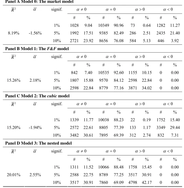
Portfolios as test assets
Table 6 presents the outputs ( , 2
R
α
) of the different time-series regressions (M0, M1, M2, and M3) that are conducted on the 100 test portfolios. All R2s are adjusted.< Insert Table 6 >
The average R2 and α and tests on the value of α are reported. On average, the best performing model appears to be the nested model (M3) if we consider the R2 as the criterion, or the market model according to the level of specification errors. The F&F and cubic premiums seem to deliver equivalent quality for pricing portfolio returns. Note that F&F produces only positive alphas when significant, indicating that this specification is more likely to produce an upward bias, while the specification using the cubic premiums regularly produces a downward bias but not systematically.
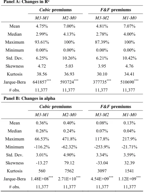
Overall, the large number of significant alphas indicates that both sets of premiums, when used in a four-factor model, produce strong model misspecification. Therefore, in this particular portfolio context, neither the F&F nor the cubic risk space can fully characterize the cross-section of test asset portfolios. Nevertheless, it has to be reminded that these portfolios are not tradable as they are formed on the basis of the statistical properties of the full time series of returns, and they are never rebalanced. The main interest of the approach with portfolio test assets lie in the study of the complementary character of the information brought by both sets of premiums. Table 7 presents descriptive statistics about the change in R² and alpha (in absolute value) brought by F&F premiums (resp. by the cubic premiums) when introduced in the market model or in the cubic risk model (resp. in
the F&F model) for the 100 portfolios over the period May 80-April 07. The added value of the cubic
risk model is represented by the columns M3-M1 (passage from the F&F to the global specification)
and M2-M0 (passage from the single factor to the cubic specification). Similarly, the added value of
the F&F model is represented by the M3-M2 and M1-M0 columns.
< Insert Table 7 here >
Panel A shows that on average, the F&F premiums add 3.5% of explanatory power to the
cubic model, while the cubic premiums add nearly 3.91% of R² to the F&F model. Moreover, both sets
of premiums add on average 11% of explanatory power to the market model. Panel B shows however that adding either the F&F or the cubic premiums to the market model increases the specification error of the model. On average, the F&F premiums decrease the absolute value of the specification error of
the cubic model. The distribution of the changes in alpha from model M2 to model M3 is heavily
We dig further in the assessment of the complementary character of the alternative sets of premiums by considering the significance rather than the magnitude of the changes. In Table 8, we examine the frequency with which each set of premiums significantly increases the explanatory power or significantly decreases the specification error of a more parsimonious specification. This semi-parametric analysis puts lower weight on the portfolios for which all models are severely misspecified. Rather, it mostly focuses on cases where the quality of information improves.
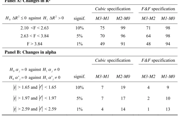
< Insert Table 8 here >
Table 8 reports the number (equal to the percentage) of significant increases in R²s brought by
cubic premiums (resp. by the F&F premiums) when introduced in the market model or in the F&F risk
model (resp. in the cubic model) for the 100 portfolios (Panel A). In Panel B, the table also displays the proportion of alphas that becomes non-significant when either the F&F or the cubic premiums are introduced in the regressions.
Panel A shows that the two sets of premiums are complementary as the F&F premiums add explanatory power to the cubic model for the majority of the portfolios (71%), and vice versa (75%).
The cubic model seems to slightly outperform the F&F premiums. First, the cubic risk premiums
complement the determination to the F&F premiums for a larger number of portfolios than the F&F model does for the cubic premiums. Second, the cubic premiums seem also to decrease the specification errors of the market model for a larger number of portfolios. They also reduce the specification error of a model made of F&F premiums.
Overall, the analysis on portfolios shows that although our premiums and the F&F factors are correlated, both sets of factors display a strong complementary character. They intend to price the same types of risks, but differ in some part of the information they contain. Moreover, both sets of premiums improve the specification of the market model. The cubic premiums slightly outperform the F&F ones.
Individual Stocks as Test Assets
Table 9 presents the outputs of the regression models M0, M1, M2, and M3 when conducted on the individual stocks.
< Insert Table 9 >
The best specified model along the R² seems to be the one that combines the F&F and the
cubic premiums. Along the specification errors criterion however, the market model is the best
premiums under-estimate it. Higher proportions of significant specification errors are found in the
cubic model than in the F&F one.
Table 10 presents descriptive statistics similar to Table 8, but this time for individual stocks. < Insert Table 10 here >
Panel A shows that both sets of empirical premiums bring on average approximately the same improvements in R² on the market model (7%). Like for the test portfolios, we emphasize the complementarities between the F&F original and cubic premiums since both add on average more than 4.8% of explanatory power to each other. From panel B, it appears that neither the F&F, nor the cubic version of the premiums is able to reduce the specifications errors of the market model.
Table 11 has a similar structure to Table 8, but applied on individual stocks as test assets. < Insert Table 11 here >
Comparatively to the F&F version, our cubic premiums bring significant complement of explanatory power to the market model for many more stocks. This result holds for all significance levels. Besides, both sets of premiums are complementary for more than 20% of the stocks at the significance level of 5 and 10%: the cubic premiums add significant explanatory power to the F&F model and vice versa.
The F&F premiums decrease significantly the specification errors of the market model for a
larger number of stocks (2,017 vs. 1,793) at a confidence level of 10%. The F&F premiums decrease also more often the specification errors of the cubic model than vice versa.
To conclude, the cubic model delivers better explanatory power when explaining either the stock or the portfolio returns. The F&F premiums produce on average less specification errors for individual stocks, while the cubic premiums outperform the F&F premiums for portfolio test assets.
IV. Non-Nested Models
This section attempts to identify the potential superiority of one set of empirical premiums (either the
F&F ones or our updated version) over the other one. We follow the literature on model specification
tests against non-nested alternatives (MacKinnon, 1983; Davidson and MacKinnon, 1981, 1984). Such tests have already been used in the financial and the macroeconomics literature28.
28 Among others, Bernanke
et al. (1986) and Elyasiani and Nasseh (1994) use non-nested models to compare
specifications of investment and U.S. money demand, respectively. Elyasiani and Nasseh (2000) contrast the performance of the CAPM and the consumption CAPM through non-nested econometric procedures. Al-Muraikhi and Moosa (2008) test the impact of the actions of the traders who act on the basis of fundamental or technical analysis on financial prices based on non-nested models.
Two tests are jointly conducted. First, the model to be tested is M1, and the alternative model M2. To test the model specification, we set up a composite model within which both models are nested. The composite model (M4) writes:
it i i i it X Z R =α ''4+β μ+(1−θ1)β ' +θ1γ ' '+ε '' (9)
Under the null hypothesis
θ
1 =0, M4 reduces to M1; ifθ
1 ≠0, M1 is rejected. Tests are conducted on the value ofθ
1. Davidson and MacKinnon (1981, 1984) prove that under H0, γˆ can be replaced by its OLS estimate from M2 so thatθ
1 andβ
are estimated jointly. This procedure is called the “J-test”. We defineβ
* =(1−θ
1)β
' so that M4 can be rewritten as follows:it i i i it X Z R '' 1ˆ' ' '' * 4 β μ β θ γ ε α + + + + = (10)
To test M2, we reverse the roles of the two models. We consider the following model (M5):
it i i i it X Z R =α ''5+β μ+θ2βˆ' +γ* '+ε '' (11)
We replace
β
'iby its estimate along M1 βˆ'i and estimate *γ
jointly with θ2. Ifθ
2 =0, M5 reduces to M2; ifθ
2 ≠0, M2 is rejected. Tests are conducted on the value ofθ
2.The following hypotheses are joinly tested on all portfolio and individual test assets: Hypothesis I: H0 :
θ
1 =0 against H1:θ
1 ≠0;Hypothesis II: H'0:
θ
2 =0 against H'1:θ
2 ≠0Each
θ
i follows a normal distribution with mean θi and volatility i. Therefore, under the null hypothesis, the statisticsi i
σ
θ follows a normal distribution N(0,1). Among the four possible scenarios,
we consider the two following cases:
• (H0,H'1), M1 is not rejected but M2 is;
• (H'0,H1), M2 is not rejected but M1 is29.
The results are presented for the portfolio and individual test assets simultaneously.
Table 12 presents descriptive statistics about the values taken by θ1(Panel A) and θ2(Panel B) across the 100 portfolios and the 11,039 individual stocks used in the analysis30.
< Insert Table 12 here >
29 Note that the rejection of
H0 does not tell anything about the validity of H0’.
30 We remove 338 observations as we require each time-series to provide a sufficient number of observations over the
For portfolios, the values taken by the mean and the median of the cross-sectional series of θ1 and θ2suggest that on average both models deliver equivalent quality in explaining portfolio returns. Any discrimination between the two models would come through the investigation of each individual portfolio. However, for individual assets, the analysis of the cross-sectional series of coefficients shows that values of θ are tilted towards the acceptance of the cubic set of empirical premiums. The average value of θ2 (76%) is indeed somewhat lower than θ1 (almost 90%). This suggests that our cubic model would be more often “accepted” than F&F model does.
To get a Table 13 examines the significance of
θ
1 andθ
2 across the portfolios and assets, for different levels of significance.< Insert Table 13 here >
The table displays, for different levels of significance, the frequency of acceptances of the
F&F model, i.e. H0 (resp. cubic model the H’0) while rejecting the cubic premiums H’1 (resp. F&F
premiums H1). For portfolios, the analysis fails to discriminate between the two models. However, as expected from the analysis of the cross-sectional time-series of the θs, the cubic version of the F&F model is more frequently accepted and the F&F premiums rejected for individual stocks than the opposite. The discrepancy is the largest at the significance level of 1%, where the cubic premiums are accepted 6.6% more often than F&F premiums.
Overall, the non-nested econometric analysis shows from the values taken by θ1 and θ2 that in most cases the F&F and the cubic models are both either accepted or rejected. For a limited subset of stocks (up to ca. one third), some discrimination between these models can be emphasized. Our cubic premiums seem to outperform the F&F specification.
V. Concluding remarks
Our paper reviews the methodology of Fama and French (1993) for creating size and BTM factors and addresses the issues surrounding their methodology when one want to apply the method to other exchange markets or price other risk fundamentals. In this way, our paper aims to tackle an important gap in the literature: how to best construct fundamental risk factors. While it has become standard practice to use the F&F method to construct multiple size and BTM portfolios and to use them in the cross-sectional asset-pricing literature to evaluate models (Daniel and Titman, 1997; Ahn et al., 2009; Lewellen et al., 2009), there is, to our knowledge, only very few articles that use such multiple portfolio sorts for pricing fundamental risk premiums.
We raise three main issues in applying the F&F methodology. First, the annual rebalancing is consumptive in long time-series which sometimes simply do not exist for small exchange markets. Moreover, this does not match with the investment horizon of the investors. Second, the independent sorting procedure underlying the formation of the 6 F&F two-dimensional portfolios causes moderate level of correlation between premiums. Replicating directly their strategy for risk fundamentals exhibiting stronger correlations would lead to empty portfolios. Finally, the breakpoints as defined along the NYSE stocks produce an over-representation of small caps in portfolios.
The main innovations of our premiums reside in a monthly rebalancing of the portfolios underlying the construction of the risk premiums, and in a conditional sorting of stocks into portfolios. The conditional sorting procedure answers the question whether there is still return variation related to the third criterion after having controlled for two risk dimensions. It consists in performing three sorts within a sort; the first two sorts are performed on control risks, while we end by the risk dimension to be priced.
We find evidence that although they are strongly correlated, the original F&F premiums and our cubic versions of the F&F premiums bring complementary information. Nevertheless, none of the alternative sets of premiums manages to reduce the specification error of the market model.
There is still some risk to be captured in both sets of premiums. As there is evidence that empirical risk premiums could be proxies for higher-order risks (Barone-Adesi et al., 2004; Chung et al., 2006, Hung, 2007; Nguyen and Puri, 2009), future research must consider the incremental value of higher-order moment related factors for benchmark models. Overall, we find that the cubic empirical model better complements the market model for explaining cross-sectional dispersion in returns than the F&F premiums.31.
We acknowledge that we do not record huge differences between both sets of factors. Therefore, we do not claim that our premiums outperform the F&F premiums. Rather, we claim that our technology (and not the premiums) outperforms the F&F method. Our objective was indeed to reformulate the F&F construction in a way that it is directly transposable to other exchange markets than the US and other risk fundamentals, and that without damaging their pricing power.
31 Our results are confirmed when the original
F&F premiums are replaced by their replication in our sample data.
References
Agarwal, V. and Naik, N. (2000) Generalized Style Analysis of Hedge Fund, Journal of Asset
Management 1(1), 93-109
Agarwal, V., Bakshi, G. and Huij, J. (2008), Higher-Moment Equity Risk and the Cross-Section of Hedge Fund Returns, unpublished working paper, Georgia State University, RSM Erasmus University, Smith School of Business.
Ahn, D.-H., Conrad, J. and Dittmar, R. F. (2009) Basis Assets, Review of Financial Studies, forthcoming.
Ajili, S. (2005), Size and Book to Market Effects vs. Co-skewness and Co-kurtosis in Explaining Stock Returns, unpublished working paper, Université Paris IX Dauphine – CEREG, presented to the Northeast Business and Economics Association, 32nd annual conference, Newport, Rhode Island, USA.
Al-Muraikhi, H. and Moosa, I. A. (2008) The Role of Technicians and Fundamentalists in Emerging Financial Markets: A case Study of Kuwait, International Research journal of Finance and
Economics 13, 77-83.
Ang, A., Liu, J. and Schwarz, K. (2009), Using Stocks or Portfolios in Tests of Factor Models, unpublished working paper, Columbia Business School, University of California, University of Pennsylvania, AFA 2009 San Francisco Meetings Paper.
Balduzzi, P. and Robotti, C. (2008) Mimicking Portfolios, Economic Risk Premiums, and Tests of Multi-Beta Models, Journal of Business and Economic Statistics 26(3), 354-368
Barone-Adesi, G., Gagliardini, P. and Urga, G. (2004) Testing Asset Pricing Models with Coskewness,
Journal of Business and Economic Statistics 22(4), 474-485.
Berk, J. (2000) Sorting Out Stocks, Journal of Finance 55(1), 407-427.
Bernanke, B., Bohn, H. and Reiss, P. C. (1986) Alternative Nonnested specification tests of time-series investment models, NBER Research Paper, 890.
Blume, M. E. (1970) Portfolio Theory: A Step Towards its Practical Application, The Journal of
Business 43(2), 152-173.
Brown, S. J. and Goetzmann, W. N. (2004), Hedge Funds with Style, Yale ICF unpublished working paper.
Carhart, M. M. (1997) On Persistence in Mutual Fund Performance, Journal of Finance 52(1), 57-82. Chung, Y. P., Johnson, H. and Schill, M. J. (2006) Asset Pricing when Returns are Nonnormal:
Fama-French Factors versus Higher-Order Systematic Comoments, Journal of Business, 79(2), 923-940. Connor, G. (1995) The Three Types of Factor Models: A Comparison of their Explanatory Power,
Financial Analysts Journal 51(3), 42-46.
Conrad, J., Cooper, M. and Kaul, G. (2003) Value vs. Glamour, Journal of Finance 59, 1969-1995. Cremers, M., Petajusto, A. and Zitzewitz, E. (2008), Should Benchmark Indices Have Alpha?
Revisiting Performance Evaluation, unpublished working paper, Yale School of Management. Daniel, K. and Titman, S. (1997) Evidence on the Characteristics of Cross Sectional Variation in Stock
Davidson, R. and MacKinnon, J. G. (1981) Several Tests for Model Specification in the Presence of Alternative Hypotheses, Econometrica 49, 781-793.
Davidson, R. and MacKinnon, J. G. (1984) Model Specification Tests based On Artificial Linear Regressions, International Economic Review 25, 485-502.
Easley, D., Hvidkjaer, S. and O’Hara, M. (2005), Factoring Information into Returns, unpublished working paper, Johnson Graduate School of Management, Cornell University, Ithaca.
Elyasiani, E. and Nasseh, A. (1994) The Appropriate Scale Variable in the U.S Money Demand: An application of Nonnested Tests of Consumption versus Income Measures, Journal of Business and
Economic Statistics 12(1), 47-55.
Elyasiani, E. and Nasseh, A. (2000) Nonnested Procedures In Econometric Tests Of Asset Pricing Theories, Journal of financial Research 23(1), 103-128.
Faff, R. (2001) An Examination of the Fama and French Three-Factor Model Using Commercially Available Factors, Australian Journal of Management 26(1), 1-18.
Fama, E. F. and French, K. R. (1992) The Cross-Section of Expected Stock Returns, Journal of
Finance 47(2), 427-465.
Fama, E. F. and French, K. R. (1993) Common Risk Factors in the Returns on Stocks and Bonds,
Journal of Financial Economics 33(1), 3-56.
Fama, E. F. and MacBeth, J. D. (1973) Risk, Return, and Equilibrium: Empirical Tests. Journal of
Political Economy 81(3), 607-636.
Fung, W. and Hsieh, D. (1997) Empirical Characteristics of Dynamic Trading Strategies: The Case of Hedge Funds, Review of Financial Studies 10(2), 275-302.
Gibson, R. and Gyger, S. (2007) The Style Consistency of Hedge Funds, European Financial
Management 13(2), 287-308.
Griffin, J. M. and Lemmon, M. L. (2002) Book-to-Market Equity, Distress Risk, and Stock Returns,
The Journal of Finance 57(5), 2317-2336.
Huberman, G., Kandel, S. and Stambaugh, R. F. (1987) Mimicking Portfolios and Exact Arbitrage Pricing, Journal of Finance 42(1), 1-9.
Hung, D. C.-H. (2007), Momentum, Size and Value Factors versus Systematic Co-Moments in Stock Returns, unpublished working paper, Durham University.
Jegadeesh, N. and Titman, S. (1993) Returns to Buying Winners and Selling Losers: Implications for Stock Market Efficiency, Journal of Finance 48(1), 65-91.
Jegadeesh, N. and Titman, S. (2001) Profitability of Momentum Strategies: An Evaluation of Alternative Explanations, Journal of Finance 56(2), 699-720.
Kat, H. and Miffre, J. (2006), Hedge Fund Performance: The Role of Non-Normality Risks and Conditional Asset Allocation, unpublished working paper, Cass Business School, City University, London Faculty of Finance.
Kole, E. and Verbeek, M. (2006), Crash Risk in the Cross Section of Stock Returns, unpublished working paper, Erasmus University Rotterdam.
Lewellen, J., Nagel, S. and Shanken, J. (2009) A Skeptical Appraisal of Asset-Pricing Anomalies.
Lintner, J. (1965) The Valuation of Risk Assets and the Selection of Risky Investments in Stock Portfolios and Capital Budgets, Review of Economics and Statistics 47(1), 13-37.
Lo, A. and MacKinlay, A. C. (1990) Data-snooping Biases in Tests of Financial Asset Pricing Models,
Review of Financial Studies 3, 431-468.
MacKinnon, J. G. (1983) Model Specification Tests against Non-nested Alternatives, Econometric
Review 2, 85-110.
Mahajan, A. and Tartaroglu, S. (2008) Equity Market-Timing and Capital Structure: International Evidence, Journal of Banking and Finance 32(5), 754-766.
Moreno, D. and Rodriguez, R. (2009) The Coskewness Factor: Implications for Performance Evaluation, Journal of Banking and Finance 33(9), 1664-1676.
Mossin, J. (1966) Equilibrium in a Capital Asset Market, Econometrica 34(4), 768-783.
Nguyen, D. and Puri, T. N. (2009) Higher Order Systematic Co-Moments and Asset Pricing: New Evidence, The Financial Review 44(3), 345-369.
Sharpe, W. F. (1964) Capital Asset Prices: A Theory of Market Equilibrium under Conditions of Risk,
Journal of Finance 19(3), 425-442.
Sharpe, W. F. (1992) Asset Allocation: Management Style and Performance Measurement, Journal of
Table 1: Descriptive statistics of the F&F and cubic market portfolios (February 1973- June 2008). m R Rm,ff Mean 0.60% 0.66% Median 0.86% 1.04% Maximum 11.28% 12.43% Minimum -23.58% -23.14% Std. Dev. 3.95% 4.33% Skewness -0.96 -0.76 Kurtosis 7.43 5.90 Jarque-Bera 315*** 144*** Correlation 99.7%
Table 1 displays descriptive statistics about the monthly returns of the F&F and the cubic market portfolios over the
Table 2: Descriptive statistics of the empirical risk premiums (May 1980-April 2007)
Panel A F&F premiums Panel B Cubic F&F premiums
SMBff HMLff MOMff SMB HML MOM Mean 0.14% 0.44% 0.79% 0.88% -0.07% 0.91% Median -0.06% 0.38% 0.90% 0.84% 0.01% 0.92% Maximum 21.96% 13.85% 18.39% 12.88% 19.15% 10.65% Minimum -16.79% -12.40% -25.06% -11.71% -14.16% -11.26% Std. Dev. 3.24% 3.16% 4.26% 3.12% 3.23% 2.71% Skewness 0.76 0.07 -0.56 0.08 0.24 -0.25 Kurtosis 11.47 5.34 9.06 5.18 8.34 5.56 Jarque-Bera 999*** 74.5*** 512*** 64.4*** 388*** 91.9*** t-stat 0.79 2.49* 3.32** 5.07*** -0.40 6.030*** # Obs 324 324 324 324 324 324
Table 2 displays descriptive statistics for size (SMB), Book-to-market (HML) and Momentum (MOM) premiums over
the period ranging from May 1980 to April 2007. Panel A presents the statistics for the empirical risk premiums of
F&F, while Panel B presents the statistics for the updated F&F premiums built along our cubic methodology. *, ** and