Do rare events explain CDX tranche spreads?
∗
Sang Byung Seo
University of Pennsylvania
Jessica A. Wachter
University of Pennsylvania
and NBER
January 29, 2015
AbstractThe CDX is an index of credit default swaps on major U.S. corporations. In the 2005– 2008 period, contracts on the CDX as a whole and on tranches of the CDX were actively traded. Senior tranches are essentially deep out-of-the-money options because they do not incur any losses until a large number of investment-grade firms default. Because of the liquidity of these contracts, their spreads provide a unique window into how the market assesses the risk of a rare disaster. We propose a model to jointly explain the spreads on each CDX tranche, as well as prices on put options and the aggregate market. Our results demonstrate the importance of beliefs about rare events, even in periods of relatively high valuation. Moreover, our results show a basic consistency in these beliefs across different asset classes.
∗Work in progress; comments welcome. Seo: [email protected]; Wachter:
[email protected]. We thank Nick Roussanov, Ivan Shaliastovich, Amir Yaron and semi-nar participants at the Wharton School for helpful comments.
1
Introduction
In both academic work and the popular press, financial engineering has been implicated as a cause of the 2008 financial crisis. One hypothesis is that complex securities were falsely given high ratings. These sold at low interest rates, allowing financial firms to take on more leverage. By making financial firms extremely sensitive to small losses, this artificially high leverage contributed to the crisis.
In this paper, we focus on securities based on an index of credit default swaps. This index is known as the CDX, and tranches on the CDX were actively traded both before and during the crisis. Accordingly, Coval, Jurek, and Stafford (2009) identify mis-pricing in these tranches, based on a model that computes risk using option prices, and fits the spreads assuming that the spread on the 5-year CDX is priced correctly. They find that spreads on the senior tranches are too low and that spreads on the junior tranches are too high, consistent with the hypothesis above. This story is questioned, however, by Collin-Dufresne, Goldstein, and Yang (2012), who argue that the focus on the 5-year spread distorts the results. Indeed, in order to price spreads at all maturities, it is necessary to allow for idiosyncratic jumps. Furthermore, a small probability of a system-wide catastrophic jump is necessary for matching overall credit spreads.
Unlike Coval, Jurek, and Stafford (2009), who use a static model that assumes default at the maturity of a bond, Collin-Dufresne, Goldstein, and Yang (2012) solve a dynamic model of structural default. They specify a stochastic discount factor and allow for both systematic and idiosyncratic jumps in asset value. However, their model is still reduced-form, and therefore disconnected from underlying risks in the economy. For example, their model allows for the specification of jump risk under the risk-neutral measure, but not the physical measure. Furthermore, they solve their model under the assumption of constant jump risk. In their calibration, however, they assume that jump risk is time-varying.
In this paper, we aim to value tranches on the CDX using a representative-agent model. We require that the model be consistent with facts about the aggregate market, and, impor-tantly, option prices, as the connection between options and credit spreads is well known. Our model allows for a catastrophic jump in prices driven by consumption (a rare disaster, as in Barro (2006) and Rietz (1988)), as well as large idiosyncratic jumps in assets covered in the CDX index. Our model also allows for the probability of both types of jumps to vary over time. We calibrate the model to match prices on index options. In order to match option prices, we use a two-factor model for the risk of rare disasters developed in earlier work (Seo and Wachter (2015)). We find that our model can explain the spreads on both CDX junior and senior spreads, while at the same time generating a reasonable fit to implied volatilities on index options. Rather than arising from mis-pricing, low spreads on senior CDX tranches could plausibly be observed in a period characterized by a low risk of a disaster. Options and equity data also point to 2005 to mid-2007 as being such a period.
2
Model
2.1
Model primitives and the state-price density
We use the two-factor stochastic disaster risk model of Seo and Wachter (2015). Namely, we assume an endowment economy with complete markets and an infinitely-lived representative agent. Aggregate consumption (the endowment) solves the following stochastic differential equation:
dCt
Ct−
where BC,t is a standard Brownian motion and NC,t is a Poisson process. The intensity of
NC,t is given by λt and assumed to be governed by the following system of equations:
dλt = κλ(ξt−λt)dt+σλ p λtdBλ,t dξt = κξ( ¯ξ−ξt)dt+σξ p ξtdBξ,t,
where Bλ,t and Bξ,t are Brownian motions (independent of each other and of BC,t).
We will assume a recursive generalization of power utility that allows for preferences over the timing of the resolution of uncertainty. Our formulation comes from Duffie and Epstein (1992), and we consider a special case in which the parameter that is often interpreted as the elasticity of intertemporal substitution (EIS) is equal to 1. That is, we define continuation utility Vt for the representative agent using the following recursion:
Vt=Et Z ∞ t f(Cs, Vs)ds, where f(C, V) =β(1−γ)V logC− 1 1−γ log((1−γ)V) . (1)
The parameter β is the rate of time preference. We follow common practice in interpreting
γ as relative risk aversion. This utility function is equivalent to the continuous-time limit (and the limit as the EIS approaches one) of the utility function defined by Epstein and Zin (1989) and Weil (1990).
As shown in Appendix A, the value function has the solution
Vt =J(Ct, λt, ξt) =
C1−γ
1−γe
a+bλλt+bξξt,
with coefficientsa, bλ andbξ given in the Appendix. In Appendix B, we show that this value
function implies the following state-price density
π = exp ηt−βb Z t λ ds−βb Z t ξ ds βC−γea+bλλt+bξξt, (2)
and risk free rate
rt=β+µ−γσ2+λtE
e(1−γ)Zt −e−γZt.
Equations for the aggregate market and index options can be found in Seo and Wachter (2015). Here, we focus on computing CDX prices.
2.2
Defaults
Let Di,t be the payout amount of firm i (i= 1,· · · , N). While we use the notation Di,t, we
intend this to mean the payout not only to the equity holders but the bondholders as well. The payout is driven by common sources of riskBct andNct that affect consumption as well,
as well as idiosyncratic sources of risk Bi,t and Ni,t. That is,
dDi,t
Di,t−
=µidt+φiσCdBC,t+ (eφiZC,t −1)dNC,t+σidBi,t + (eZi,t−1)dNi,t
| {z }
idiosyncratic risk
.
The processes Bi,t, fori= 1, . . . , N, are independent Brownian motions. The processes N it
have Poisson increments. To avoid a multiplicity of state variables, we assume that the intensity of the Poisson processes are jointly driven by χt. However, conditional on χt, the
incrementsdNit are independent. We assume that χfollows a CIR process:
dχt =κχ( ¯χ−χt)dt+σχ √
χtdBχ,t.
This structure allows for exposure to disasters (through Nct), as well as to large
idiosyn-cratic events. Note that, as is usual in the literature on endowment economies, these firms have greater exposure to disasters than the consumption process itself, as indicated by the parameter φ.1
1Note however that φ does not have the interpretation of financial leverage, as D
it is total payout.
However, φ > 1 is still possible in the presence of labor income. Our calibration of φ will reflect the interpretation ofDitas including interest as well as dividends.
Let Ai,t denote the total value of firm i (the equity plus the debt). That is Ai,t is the
price of the payout stream:
Ai,t =Et Z ∞ t πs πt Di,sds . (3)
We denote Gi(λt, ξt, χt) as the asset-payout ratio (Ai,t/Di,t) of firm i. We show that this
ratio is expressed as
Gi(λt, ξt, χt) =
Z ∞
0
exp (ai(τ) +biλ(τ)λt+biξ(τ)ξt+biχ(τ)χt)dτ, (4)
where ai(τ), biλ(τ), biξ(τ), and biχ(τ) solve the system of ordinary differential equations
derived in Appendix C.
We define default as the event that a firm’s value falls below a threshold following Black and Cox (1976) and many subsequent studies. LetAi,B denote the threshold for firmi. Then
the default time is the random variable defined as
τi = inf{t:Ai,t ≤Ai,B}.
We let Ri denote the recovery rate of firm i upon default.
2.3
CDX pricing
CDX indices are baskets of equally-weighted individual credit default swap (CDS) contracts for a set of large U.S. investment-grade firms.2 We will let N denote the number of firms
in the index (for all CDX indices thus far, the number of firms has been 125). Taking a $1
2Each CDS contract involves two parties: protection buyer and protection seller. The protection seller
provides the protection buyer an insurance against a credit event of the reference entity (specified in a CDS contract). Thus, the protection buyer pays a series of insurance premiums to the protection seller. In return, if the reference entity experiences a credit event, the protection seller compensates the loss of the protection buyer, either by purchasing the reference obligation from the protection buyer at its par value (physical
protection sell position on the CDX index can be viewed as taking protection-sell positions with notional amounts $1/N on all N individual CDS contracts in the index.
We first develop formulas for the payoffs and pricing of the sell and protection-buy positions on the index. Assume a $1 notional amount. If firm i defaults, then the protection seller pays the protection buyer N1(1−Ri). The cumulative loss process on the
index, Lt, can therefore be expressed as
Lt = 1 N N X i=1 1{τi≤t}(1−Ri). (5)
The value of the cash flows paid by the protection seller is given by
ProtCDX = ˜E Z T 0 e−R0trsdsdL t . (6)
where ˜E denotes the expectation taken under the risk-neutral measure andrt is the riskfree
rate.3
In the CDX contract, the protection buyer makes quarterly premium payments that, over the course of a year, add up to a pre-determined spread S. If a firm defaults, the size of premium payments goes down because the outstanding notional amount of the CDS contract is reduced by N1. Let nt denote the fraction of firms that have defaulted as of time t:
nt= 1 N N X i=1 1{τi≤t}. (7)
For a given spreadS, the expected present value of cash flows paid by the protection buyer is given by PremCDX(S) = SE˜ " M X m=1 e−R0tmrsds(1−nt m)∆m+ Z tm tm−1 e−R0ursds(u−tm−1)dns # , (8) where 0 =t0 < t1 <· · ·< tM are premium payment dates,S is the premium rate (premium
payment per unit notional), and ∆m = tm−tm−1 is the m-th premium payment interval.4
3The risk-neutral measure and riskfree rate are implied by the model in Section 2.1.
4IfT is the maturity of the CDS contract (in years), the total number of premium paymentsM is equal
Note that if a default occurs between two premium payment dates, the protection buyer must pay the accrued premium from the last premium payment date to the default date. This is taken into consideration as the second term in the expectation of equation (8).
To simplify notation, we have assumed above that the contracts originate at time 0. Because the model is stationary, this assumption is without loss of generality. The CDS spread SCDX is defined as the value of the premium rate that equates the protection and
premium legs (i.e. PremCDX(SCDX) =ProtCDX). That is, SCDX is determined by
SCDX =ProtCDX/PremCDX(1).
Appendix D shows how to compute the spread, which is a function of the state variables λ,
ξ and χ.
2.4
CDX tranche pricing
Each tranche is defined by its “attachment point” and “detachment point.” The attachment point refers to the level of subordination of the tranche, and the detachment point is the level at which the tranche loses its entire notional amount. For example, consider the tranche with a 10% attachment point and 15% detachment point. The protection seller of this tranche does not experience loss until the the entire pool (i.e. the CDX index) accumulates more than a 10% loss. After the 10% level, every loss the pool experiences “attaches” to the tranche. That is, the protection seller of the tranche should compensate the loss after 10%. If the loss of the pool reaches the detachment point of 15%, the protection seller loses the entire notional amount and no longer needs to take the loss of the pool. (i.e. further loss “detaches” from the tranche.)
The detachment of a tranche is the attachment of the next (higher) tranche. Suppose that there areJ tranches based on the CDX index. We denoteKj−1 as the attachment point
first tranche (K0) is equal to 0 and the detachment point of the last tranche (KJ) is equal
to 100%.
To properly understand the mechanism of tranche products, it is important to see that a default in the pool not only affects the most junior tranche but also the most senior tranche. To illustrate this, consider a simple case where (1) the entire pool consists of 100 CDS contracts, each of which has $1 notional amount, and (2) there are only two tranches: 0-50% and 50-100% tranches based on the pool. How does an event of one firm’s default in the pool affect the two tranches, assuming that the defaulted firm’s recovery rate is 40%? This event affects both the 0-50% and 50-100% tranches. Since the recovery rate is 40% and each CDS contract is with $1 notional, the loss amount of the pool is $0.6. Since the 0-50% tranche is the most junior tranche, the protection seller of this tranche takes this loss. The difference between $1 (notional amount of the defaulted CDS contract) and $0.6 (loss amount from the defaulted CDS contract) reduces the notional amount of the 50-100% tranche exactly by $0.4.5
The reason why the notional amount of the most senior tranche decreases is straight-forward if we consider a case for funded CDO products: if a default occurs in the pool, the loss amount goes to the most junior tranche holder, and the recovery amount from the default goes to the most senior tranche holder as an early redemption. That is, the notional amount of the senior tranche is reduced by the redemption amount. Since CDX tranches are unfunded CDO products, which do not require initial investments, there is no actual early redemption in cash as the case for funded CDO products, but still the notional amount of the most senior tranche is reduced by the recovery amount.
In sum, a default in the pool affects both the most junior tranche (by incurring loss)
5This is not a loss to the protection seller of this tranche. The notional amount simply reduces to $49.6.
This means that the maximum loss the protection seller can experience is $49.6. Thus, the protection seller receives insurance premium based on the reduced notional amount $49.6.
and the most senior tranche (by reducing its notional amount). Keeping this in mind, we derive the expressions for the loss and recovery amount of the j-th tranche as a fraction of the notional amount of the tranche (Kj −Kj−1):
Tj,tL = min{Lt, Kj} −min{Lt, Kj−1}
Kj −Kj−1
Tj,tR = min{nt−Lt,1−Kj−1} −min{nt−Lt,1−Kj}
Kj−Kj−1
. (9)
Let ProtTran,j be the protection leg of the j-th CDX tranche. The expression for
ProtTran,j is the same as the one forProtCDX except that the integral is with respect to the
tranche loss (Tj,tL) rather than the entire pool loss (Lt):
ProtTran,j = E˜ Z T 0 e−R0trsdsdTL j,t .
LetPremTran,j(U, S) be the premium leg of thej-th CDX tranche when the protection buyer
pays quantity U up front and quarterly premiums with premium rate S. Since insurance premiums accrue based on the outstanding notional amount (which can be decreased from 100% due to a tranche loss (Tj,tL) or a tranche recovery (Tj,tR)), we can show that
PremTran,j(U, S) = U +SE˜ " T f X m=1 e−R0trsds Z tm tm−1 1−Tj,tL −Tj,tRds # .
In our sample period, the entire CDX pool has been partitioned into 6 tranches, which are traded as separate products: 0-3%, 3-7%, 7-10%, 10-15%, 15-30% and 30-100% tranches. The first tranche is called the equity tranche and the second tranche is called the mezzanine tranche. The four remaining tranches are called senior tranches, and, in particular, the last (most senior) tranche is called the super senior tranche.
Except for the equity tranche, tranches are traded with zero upfront amount. Thus, for each of those tranches, the CDX tranche spread (STran,j) is determined by
The equity tranche is traded with the upfront amount, fixing the premium rate at 500bp. Thus, the upfront amount for the equity tranche (UTran,j) is determined by
UTran,j =ProtTran,j−PremTran,j(0,0.05) if j = 1.
Again, in Appendix D, we show that the spread and upfront amount for CDX tranches can be calculated as a function of the state variables λ, ξ and χ.
3
Evaluating the model
3.1
Data
Our analysis requires the use of pricing data from the options and CDX markets. First, our sample of options consists of implied volatilities on S&P 500 European put options. We collect our sample from OptionMetrics, which provides the time series and the cross section of implied volatilities on individual stocks and equity indices from January 1996 to December 2012. To construct monthly time-series of implied volatility smiles, we pick observations using the data from the Wednesday of every option expiration week. Following Seo and Wachter (2015), we apply standard filters to extract contracts with meaningful trade volumes and prices. The implied volatility smile for each date can be obtained by regressing implied volatilities on a polynomial in strike price and maturity.
CDX is a family of credit default swap (CDS) indices, mainly covering firms and enti-ties in North America. Among many different indices, we focus on the CDX North America Investment Grade (CDX NA IG) index, which is the most actively traded. This index is com-posed of 125 equally weighted CDX contracts on representative North American investment grade firms.
Unlike equity indices, CDS indices have expiration dates because they consist of multiple contracts with certain maturities. Three-, five-, seven-, and ten-year indices are typically
traded. Since each index has an expiration date, the time-to-maturity decays. For this very reason, CDX indices roll every 6 months in March and September. That is, every March and September, a new series of indices is introduced to the market and the previous series becomes off-the run. There have been a total of 20 series to date.
Our data set contains daily market pricing information on CDX NA IG indices from MARKIT. Although the first series of CDX (CDX1) was traded from September 2003, MARKIT provides five- and ten-year data from series 5 and seven-year data from series 6. We extract the monthly time series of on-the-run series using the same dates for our option sample. We only use on-the-run series data because the latest series are the most liquid.
In this paper, our period of interest is from October 2005 to September 2008, which corresponds to CDX series 5 to 10. We divide our sample period into two sub-periods: pre-crisis and post-pre-crisis. Pre-pre-crisis sample is from October 2005 to September 2007 (CDX5 to CDX8). Post-crisis sample is from October 2007 to September 2008 (CDX9 to CDX10). Note that our sample period ends before SNAC was introduced. Therefore we do not need to consider changes in the trading convention in the market. In our entire sample, CDX index and all tranches are quoted in terms of spreads and the equity tranche is quoted in terms of upfront amount with 500bps fixed running spread.
3.2
Calibration
The parameter values for aggregate consumption, market dividends, and for utility are shown in Table 1. To ensure that our model can match consumption data, aggregate market data and data on index put options, we use similar parameter values as in Seo and Wachter (2015). That is, we choose risk aversion of 3, and EIS equal to 1 (which allows for closed-form solutions), and standard parameters for temporal discounting, normal-times consumption
growth, normal-times consumption volatility, and the leverage for the dividend claim. For convenience, rather than using the multinomial distribution of Barro and Urs´ua (2008), we assume a power law distribution with a minimum value of 10% and a tail parameter of 7. This is a reasonable approximation to the multinomial distribution (Barro and Jin (2011)), but is slightly more conservative in that the tail probabilities of very bad events are lower. To keep other quantities in the model the same, we make a slight adjustment to the volatility parameters. Otherwise, parameter values for the λt and ξt processes are the same as in Seo
and Wachter (2015).
Table 2 reports parameter values for the individual firm dynamics. Collin-Dufresne, Goldstein, and Yang (2012) estimate the asset beta of the portfolio of firms in the CDX index as 0.56-0.66, the idiosyncratic volatility as 0.179-0.192, and the leverage ratio as 29-37%. To be consistent with their estimates, we setφi, σi, and the leverage ratio equal to 1.456, 0.19,
and 32%, respectively. The recovery rate upon default is assumed to be 40% during normal times but 20% during disasters. As recent literature suggests, we set the default boundary much smaller than the leverage ratio. Specifically, we set the default boundary to 60% of the leverage ratio following Collin-Dufresne, Goldstein, and Yang (2012).
Lastly, we assume that the long run mean of the idiosyncratic jump intensity process ( ¯χ) is 1.5%, the mean reversion (κχ) is 0.1, and the volatility parameter (σχ) is 0.05. Since
we want to capture the possibility of sudden defaults of individual firms using idiosyncratic jumps, the consequences of jumps are severe. That is, we setZi so that the firm value drops
75% when idiosyncratic jumps happen.
3.3
Choice of state variables
A standard approach to comparing an endowment economy model with the data is to sim-ulate population moments and compare them with data moments. In a model with rare
disasters, this may not be the right approach if one is looking at a historical period that does not contain a disaster. An alternative approach is to simulate many samples from the stationary distribution implied by the model, and see if the data moments fall between the 5th and 95th percentile values simulated from the model. For this study, this approach is not ideal either, for two reasons. First, the short length of the CDX time series will likely mean that the error bars implied by the model will be very wide. Thus this test will have low power to reject the model. Second, unlike stock prices which are available in semi-closed-form, and options, which are available up to a (hard-to-compute, but nonetheless one-dimensional) integral, CDX prices must be simulated for every draw from the state variables. Thus the simulation approach is computationally infeasible.
For these reasons, we adopt a different approach. We use three time series from the data to infer time series for our three state variables. We then generate predictions for the remaining quantities in the data based on this series of state variables. We are thus setting up a more stringent test than endowment economy models are usually subject to. Namely, we are asking that the model match not only moments, but the actual time series of variables of interest.
In the model, CDX and CDX tranche prices are determined by all three state variables
λt, ξt, and χt while option prices are determined by the first two. For each date, we back
out the values of the state variables so that the model matches (1) the five-year 15-30% tranche spread, (2) the five-year 0-3% tranche upfront amount, and (3) the one-month at-the-money (1M ATM) implied volatility. The spread senior tranche is almost entirely driven by catastrophic risk, and so it is a good source of information for rare-disaster intensity
λt. The equity tranche, on the other hand, is particularly sensitive to idiosyncratic risk χt.
Finally, ξt is a major determinant of stock market volatility , which can be proxied for by 1
and option prices.
3.4
Results
Our goal in this paper is not only to match CDX spreads, but to do so in a way that is consistent with asset prices more broadly. In Seo and Wachter (2015), we show that our model, calibrated at these parameters is capable of matching the mean and volatility of Treasury bills and of excess stock returns. Thus, at these parameters, the model can resolve the riskfree rate, equity premium, and volatility puzzles, even with a low risk aversion for the representative agent. The model generates very little predictability of consumption growth (in samples without disasters there is no consumption growth predictability). Moreover, excess stock returns, are predictable, consistent with the data. In samples without disasters, consumption growth volatility matches the low volatility of the postwar sample in the U.S. Because the pricing of CDX products is closely tied to aggregate volatility, matching the volatility puzzle is particularly important. These results show that our model explains aggregate stock market volatility without counterfactually introducing volatile or predictable consumption, or volatile interest rates.
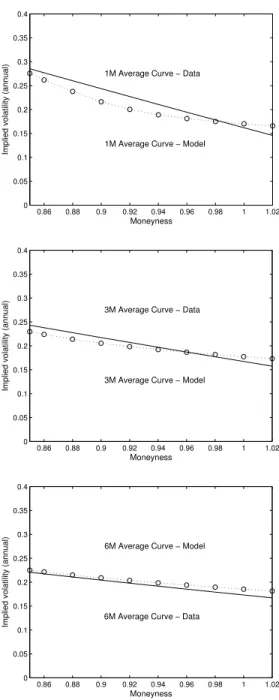
The link between put options and the pricing of default risk is well-known, so verifying the ability of the model to match option prices is also important. While options are the subject of Seo and Wachter (2015), we check that this is still the case, given that we use a different algorithm to back out the values of the state variables. Indeed, Figure 1 verifies that the model can match the implied volatility smirk at the 1-month, 3-month, and 6-month maturities. As Seo and Wachter (2015) discuss, the model’s ability to match option prices arises in part from the fact that it can match the volatility of stock returns. Moreover, out-of-the-money put options are a particularly good hedge against increases in the risk of a disaster, leading implied volatilities to be higher than realized volatilities. These affects
persist for 6-month options (Panel C) because the model endogenously generates long-horizon skewness in asset returns.
We now turn to the pricing of CDX products. Figure 2 shows average spreads for the index as a whole, and for various tranches at maturities of 5, 7, and 10 years (for the equity tranche, we show the upfront amount because the spread is fixed). The model prices the 5-year spreads almost exactly. One one level this is not surprising, as the state variables are chosen to match the upfront amount of the equity tranche and the spread of 15-30% tranche. However, it is not automatic that the model would match the spreads of all tranches in between, as well as the CDX index as a whole. Moreover, the debate between Coval, Jurek, and Stafford (2009) and Collin-Dufresne, Goldstein, and Yang (2012) pertains to the 5-year spread. Coval, Jurek, and Stafford (2009) find that the spreads of all tranches reported in Figure 2 except the equity tranche are too low in the data compared with their model. In our model, the 5-year spreads are very close to the data for all tranches.
We go a step beyond Coval, Jurek, and Stafford (2009) and Collin-Dufresne, Goldstein, and Yang (2012) and report data and model spreads for longer-term CDX contracts in Figure 2. Our model is also able to explain the average spreads for the 7-year contracts. Though the model was not fit to these contracts, the spreads on the total CDX index are matched almost exactly. For 10-year contracts, the model predicts spreads that are slightly higher than in the data, with the difference being most notable for the 10-15% and 15%-30% tranche. However, this difference is small compared to the mispricings reported by Coval, Jurek, and Stafford (2009), and similar in magnitude to the errors of the preferred model in Collin-Dufresne, Goldstein, and Yang (2012) for the 5-year spread.
As Collin-Dufresne, Goldstein, and Yang (2012) show, the prices of CDX contracts change dramatically during the time period of interest. Moreover, results in Coval, Jurek, and Stafford (2009) are (naturally) in reference to the pre-crisis period. The puzzle noted by
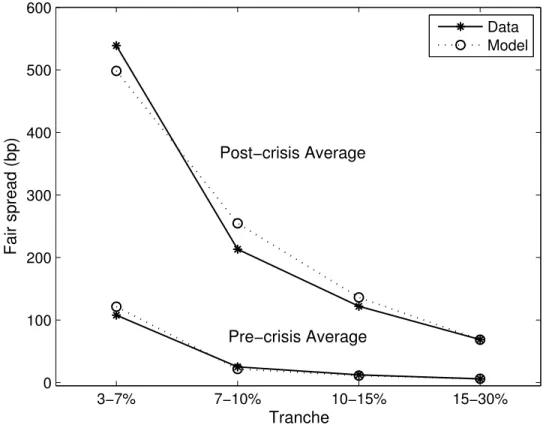
Coval et al is that average spreads on all but the most junior tranche were too low. When data for the crisis is included, spreads are higher; perhaps this is the reason why we can match average spreads in Figure 2. To test this possibility, we split the sample into pre- and post-crisis periods. 6 The solid lines in Figures 3–5 show average tranche spreads in the data
when the sample is split in this way. The financial crisis lead to a dramatic increase in spreads for all tranches from the mezzanine to senior level, and for all maturities. Consider the 5-year spreads, shown in Figure 3. For the 15-30% senior tranche, the average spread went from less than 10 basis points to close to 70 basis points. At the other end of the seniority spectrum, for the 3-7% mezzanine tranche, the average spread increased from about 100 basis points to 500 basis points. Given that the state variables are chosen to match the time series of the senior 5-year tranche, it is not surprising that this data point is matched exactly for both the pre- and post-crises periods. However, the state variables were not chosen to match the other tranches (the equity tranche will be discussed later), but the model fits these very well. The reason the model is able to capture the shift in average spreads is because it allows for time-varying probabilities of catastrophic economy-wide events, as well as idiosyncratic jumps. These possibilities are built into the dynamics of the model. In contrast, Collin-Dufresne, Goldstein, and Yang (2012) assume constant jump intensities but allow the parameters to shift over time to match the data, interpreting these as structural breaks. Their structure, however, assumes that investors do not build the possibility of such breaks into the model.
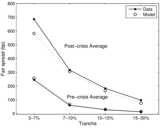
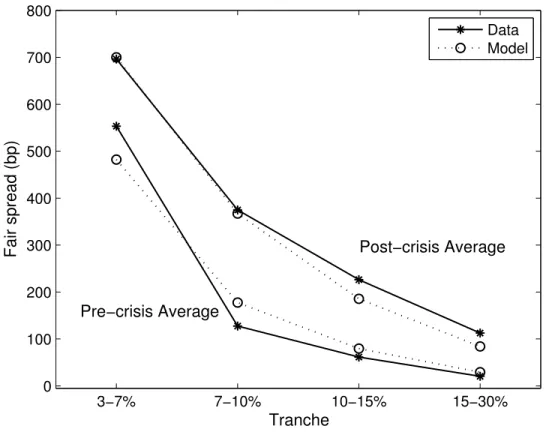
Figures 4 and 5 show 7 and 10-year tranche spreads also increase dramatically, though less than the 5-year spread. This is sensible, economically, as it indicates the beliefs of investors that the stresses firms faced during the crisis were unlikely to be permanent. Such mean reversion in disaster probabilities is built into our model, and explains why our model
6The pre-crisis period is defined as ending in September 2007, as in Collin-Dufresne, Goldstein, and Yang
(2012). While this may seem an early date for the financial crisis, the time series of CDX spreads do undergo a dramatic change at this time.
can capture the change in average spreads for these maturities, despite the fact that the state variables were not chosen based on these maturities at all.
Finally, Figures 6–8 show the actual time series of tranche spreads in the model and in the data. The solid lines, showing the data, illustrate the substantial change that these prices undergo beginning in late 2007. Consider the time series for 5-year contracts (Figure 6). After a period of relatively low spreads, spreads rose and became much more volatile. The degree to which the activity in the CDX market anticipated the broader financial crisis is interesting. An initial uptick in the level of spreads occurred in late 2007. Spreads fell slightly, but they did not return to their previous levels. Then, beginning in early 2008, spreads rose steadily to several orders of magnitude beyond anything that had been seen prior to September 2007. Spreads fell substantially, only to rise again in late 2008. This pattern holds for all tranches except for the equity tranche; it was relatively expensive to insure this tranche even early in the sample, and, while the patterns are the same, the difference in the crisis period is much less notable.
Figure 7 and 8 show the time series for the 7- and 10-year contracts. Similar patterns are apparent as in the 5-year contracts, with several important qualifications. First, as noted previously, the increase around the crisis was smaller in magnitude for 7-year as compared with 5-year contracts, and smaller still for 10-year contracts. The differences in maturity are most apparent at the junior tranches. Indeed, for the 10-year equity tranche, the crisis appears to have had little effect.
One pervasive narrative of the financial crisis focuses on a massive liquidity disruption that led to widespread mispricing, especially in structured debt products like those based on CDX tranches. This paper is based on another narrative that emphasizes changes in investor beliefs about rare events. These narratives are not mutually exclusive, as many models have emphasized the link between liquidity events and subsequent economic declines. In this
paper, however, it is investor beliefs alone that drive prices. Our intention is not to rule out other models, but simply to point out that there are some features of the data that support the view that prices on CDX products accurately reflected investor beliefs at the time. While all the products moved to a certain extent in tandem, we see much less of a change in the longer-term contracts as compared with the shorter-term contracts. This suggests the view of investors that the crisis would ultimately be short-lived. Moreover, senior tranches were far more affected than junior tranches, reflecting the fact that what had changed was primarily a view of catastrophic risk, not the idiosyncratic risk of firms.
Our model formalizes this intuition. A basic test of the plausibility of the model is that we are able, at some value of the state variables, to match the time series of prices for equity and senior tranches for 5-year contracts. Figure 6–8 show that, in addition to these, the model can match the time series of prices for the other tranches, and for other maturities. Though it is not calibrated to the longer-term contracts, the mean reversion that is built into the model allows it to price these as well. Thus both the low levels of the spreads on senior tranches prior to the crisis, as well as the much higher spreads during the crisis can be explained within a single rational and frictionless framework.
4
Conclusion
CDX senior tranches are analogous to extremely deep out-of-the-money options on the US economy because they do not incur any loss until a highly significant number of investment grade firms go into default. In this sense, CDX senior tranche spreads are an important source of information about the probability of catastrophic events. In this paper, we utilize this information to study equilibrium-based asset pricing models. Specifically, we focus on rare disaster models since we believe that the large, infrequent shocks are a natural choice to generate positive prices for extremely bad states.
We extend the two-factor stochastic disaster risk model of Seo and Wachter (2015) to explain the characteristics of CDX and CDX tranche spreads over different maturities in both the pre-crisis and the post-crisis samples. Our model can explain the equity and option markets along with the CDX market, which emphasizes the importance of beliefs about rare disasters in the asset markets.
We also point out that senior tranche spreads are very crucial source to see how the market assesses the risk of rare disasters. In this sense, our analysis potentially provides an alternative to the conventional Barro-Ursua calibration of rare disasters.
Appendix
A
Value function
We note that the state variables in the economy are Ct,λt, andξt. Since the value function
is homogeneous of degree (1−γ) in consumption and the EIS is equal to 1, we conjecture the value functionJ(C, λ, ξ) is given by
J(C, λ, ξ) = C
1−γ
1−γe
a+bλλ+bξξ. (A.1)
At equilibrium, the continuation utility is equal to the value function under the optimal policies:
Vt=J(Ct, λt, ξt).
This optimality condition implies that
f(C, V) = β(1−γ)V logC− 1 1−γlog [(1−γ)V] = βV log C1−γ (1−γ)V = −βV(a+bλλ+bξξ), A By differentiating J(C, λ, ξ), we obtain ∂J ∂C = (1−γ) J C, ∂2J ∂C2 =−γ(1−γ) J C2, ∂J ∂λ = bλJ, ∂2J ∂λ2 =b 2 λJ, ∂J ∂ξ = bξJ, ∂2J ∂ξ2 =b 2 ξJ. (A.2)
Applying Ito’s Lemma to J(C, λ, ξ) with conjecture (A.1) and derivatives (A.2): dVt Vt− = (1−γ)(µCdt+σCdBC,t)− 1 2γ(1−γ)σ 2 Cdt +bλ κλ(ξt−λt)dt+σλ p λtdBλ,t + 1 2b 2 λσ 2 λλtdt +bξ κξ( ¯ξ−ξt)dt+σξ p ξtdBξ,t + 1 2b 2 ξσ 2 ξξtdt+ (e(1−γ)ZC,t−1)dNC,t. (A.3) By adding Rt
0f(Cs, Vs)ds on both sides of (A.3), we obtain
Vt+ Z t 0 f(Cs, Vs)ds =Et Z ∞ 0 f(Cs, Vs)ds . (A.4)
By the law of iterative expectations, the left-hand side of (A.4) is a martingale. Thus, the sum of the drift and the jump compensator of (Vt+
Rt
0 f(Cs, Vs)ds) equals zero. That is,
0 = (1−γ)µC − 1 2γ(1−γ)σ 2 C+bλκλ(ξt−λt) + 1 2b 2 λσ 2 λλt+bξκξ( ¯ξ−ξt) + 1 2b 2 ξσ 2 ξξt +λtE e(1−γ)ZC,t−1−β(a+b λλt+bξξt). (A.5)
By collecting terms in (A.5), we obtain
0 = (1−γ)µC− 1 2γ(1−γ)σ 2 C +bξκξξ¯−βa | {z } =0 +λt −bλκλ+ 1 2b 2 λσ 2 λ+E e(1−γ)ZC,t−1−βb λ | {z } =0 +ξt bλκλ−bξκξ+ 1 2b 2 ξσ 2 ξ −βbξ | {z } =0 .
Solving these equations gives us a = 1−γ β µC− 1 2γσ 2 C + bξκξ ¯ ξ β bλ = κλ+β σ2 λ − s κλ+β σ2 λ 2 −2E e(1−γ)ZC,t−1 σ2 λ bξ = κξ+β σ2 ξ − v u u t κξ+β σ2 ξ !2 −2bλκλ σ2 ξ ,
where we have chosen the negative root based on the economic consideration that when there are no disasters, λ and ξ should not appear in the value function. Namely, for ZC,t = 0,
bλ =bξ= 0. Lastly, note that these results verify the conjecture (A.1).
B
The state-price density
By Duffie and Skiadas (1994), the state-price densityπt can be written as
πt = exp Z t 0 ∂ ∂V f(Ct, Vt)ds ∂ ∂Cf(Ct, Vt). (B.1)
By differentiating equation (1) with respect to C and V, we can show that
∂ ∂Cf(Ct, Vt) = β(1−γ) Vt Ct =βCt−γea+bλλt+bξξt ∂ ∂V f(Ct, Vt) = βlog C1−γ (1−γ)V −β =η−βbλλt−βbξξt, where η=−βa−β.
Therefore, it follows that the state-price density can be expressed as
πt= exp ηt−βbλ Z t 0 λsds−βbξ Z t 0 ξsds βCt−γea+bλλt+bξξt.
Furthermore, by applying Ito’s Lemma to equation (2), we derive the following stochastic differential equation: dπt πt− =−β−µC+γσC2 −λtE e(1−γ)ZC,t−1−νEebλZλ,t −1 dt −γσCdBC,t+bλσλ p λtdBλ,t+bξσξ p ξtdBξ,t + (e−γZC,t−1)dN C,t+ (ebλZλ,t−1)dNλ,t. (B.2)
At equilibrium, the sum of the drift and the jump compensator of the state-price density growth must equal the riskfree rate multiplied by -1. It thus follows that the riskfree rate is given by
rt=β+µ−γσ2+λtE
e(1−γ)Zt −e−γZt.
C
Individual firm value dynamics
LetHi(Di,t, λt, ξt, χt, s−t) denote the time-t value of firm i’s payoff at time s. That is,
Hi(Di,t, λt, ξt, χt, s−t) =Et πs πt Di,s .
We conjecture that Hi(·) has the following functional form:
Hi(Di,t, λt, ξt, χt, τ) =Di,texp (ai(τ) +biλ(τ)λt+biξ(τ)ξt+biχ(τ)χt).
To verify this conjecture, I apply Ito’s lemma to the process πtHi(Di,t, λt, ξt, χt, s−t) and
derive its conditional mean (which is the sum of its drift and jump compensator). The conditional mean of this process always equals zero because the process is a martingale.7
7Equation (C.1) implies thatπ
tHi(Di,t, λt, ξt, χt, s−t) =Et[πsDi,s]. It is straightforward thatEt[πsDi,s]
This zero mean condition provides the system of ODEs for ai(τ), biλ(τ), biξ(τ), and biχ(τ):
a0i(τ) = −β−µC −γ(φi−1)σ2C+µi+biξ(τ)κξξ¯+biχ(τ)κχχ¯
+νEe(bλ+biλ(τ))Zλ,t+biχ(τ)Zχ,t−ebλZλ,t
b0iλ(τ) = −biλ(τ)κλ+ 1 2biλ(τ) 2σ2 λ+bλbiλ(τ)σλ2+E e(φi−γ)ZC,t −e(1−γ)ZC,t
b0iξ(τ) = biλ(τ)κλ−biξ(τ)κξ+
1 2biξ(τ) 2σ2 ξ +bξbiξ(τ)σξ2 b0iχ(τ) = −biχ(τ)κχ+ 1 2biχ(τ) 2σ2 χ+E eZi,t −1. Therefore, equation (3) can be written as
Ai,t = Z ∞ t Hi(Di,t, λt, ξt, χt, s−t)ds = Di,t Z ∞ t
exp (ai(s−t) +biλ(s−t)λt+biξ(s−t)ξt+biχ(s−t)χt)ds
= Di,t
Z ∞
0
exp (ai(τ) +biλ(τ)λt+biξ(τ)ξt+biχ(τ)χt)dτ.
This subsequently implies that that the asset-payout ratio (Gi =Ai,t/Di,t) is expressed as a
function of three state variables as can be seen in equation (4).
D
Pricing of CDX products based on the model
In this appendix, we provide our approach for pricing CDX products (the CDX index and its tranche products) based on our equilibrium model. To make the computation tractable, we discretize the premium and protection legs of each product by assuming that defaults occur on average in the middle of premium payment dates (see, e.g., Mortensen (2006)) (Section D.1). This discretization is relatively accurate because premium payment interval ∆m = tm −tm−1 is relatively small (∆m = 0.25) since premium payments are quarterly.
Then, we express these discretized legs (ProtCDX, PremCDX, ProtTran,j, and PremTran,j)
in terms of four expectations under the physical measure (Section D.2). We calculate these four expectations using a simulation-based approach. (Section D.3).
D.1 Discretization of pricing formulas
First consider the discretization of the premium leg (ProtCDX) and the premium leg (PremCDX)
for CDX pricing. of a CDX contract derived in Section 2.3. With the discretization assump-tion explained above, it follows that
ProtCDX = E˜ Z T 0 e−R0trsdsdLt ' M X m=1 ˜ Ehe−R0tm−∆m/2rsds(L tm −Ltm−1) i = M X m=1 ˜ Ehe−R0tm−∆m/2rsdsLt m i − M X m=1 ˜ Ehe−R0tm−∆m/2rsdsLt m−1 i .
Since ∆m is small, the risk-free rate is unlikely to change much between timetm−∆m/2 and
tm. Therefore, we can approximate
Z tm
tm−∆m/2
rsds'
1
2∆mrtm.
which allows us to further simply the protection leg (ProtCDX) as
ProtCDX ' M X m=1 n ˜ Ehe12∆mrtme− Rtm 0 rsdsLt m i −E˜he−12∆mrtm−1e− Rtm−1 0 rsdsL tm−1 io .
We discretize the premium leg (PremCDX(S)) using the same assumption:
PremCDX(S) = SE˜ " M X m=1 e−R0tmrsds(1−nt m)∆m+ Z tm tm−1 e−R0ursds(u−tm−1)dns # ' S M X m=1 ∆mE˜ e−R0tmrsds(1−n tm) +e −Rtm−∆m/2 0 rsdsntm−ntm−1 2 .
Since ∆m/2 is small, we further approximate this expression as
PremCDX(S) ' S M X m=1 ∆mE˜ e−R0tmrsds 1−1 2ntm− 1 2ntm−1 = S M X m=1 ∆m H0(tm)− 1 2 ˜ E h e−R0tmrsdsn tm i − 1 2 ˜ E h e−R0tmrsdsn tm−1 i ' S T f X ∆m H0(tm)− 1 ˜ Ehe−R0tmrsdsnt i − 1E˜he−∆mrtm−1e− Rtm−1 0 rsdsn t − i .
whereH0(τ) = H0(λ, ξ, τ) is the price of the default-free zero-coupon bond with maturityτ,
which we derive in Appendix E.
While nearly all pricing formulas for credit derivatives under a reduced-form setup assume that interest rates are uncorrelated with defaults, we cannot make this simplifying assump-tion. This is because the systematic risk under our equilibrium model simultaneously affects both interest rates and the likelihood of defaults.
With the same discretization approach, we also obtain the discretization of the premium leg (ProtTran,j) and the premium leg (PremTran,j(U, S)) for CDX tranche pricing. It is
straightforward to show that
ProtTran,j ' T f X m=1 ˜ Ehe−R0tm−∆m/2rsds(TL j,tm −T L j,tm−1) i ' T f X m=1 n ˜ E h e12∆mrtme− Rtm 0 rsdsTL j,tm i −E˜ h e−12∆mrtm−1e− Rtm−1 0 rsdsTL j,tm−1 io and PremTran,j(U, S) ' U+S T f X m=1 ∆mE˜ " e− Rtm 0 rsds (1−TL j,tm−T R j,tm) + (1−T L j,tm−1−T R j,tm−1) 2 # ' U+S T f X m=1 ∆m H0(tm)− 1 2E˜ h e−R0tmrsdsTL j,tm i − 1 2E˜ h e−R0tmrsdsTR j,tm i −1 2 ˜ E h e−∆mrtm−1e− Rtm−1 0 rsdsTL j,tm−1) i − 1 2 ˜ E h e−∆mrtm−1e− Rtm−1 0 rsdsTR j,tm−1 i .
D.2 Pricing formulas in terms of four expectations
For notational convenience, let X0 denote the state vector at time 0, namely,
X0 = λ0 ξ0 χ0 .
We also define the following four expectations: EDR(u, t, X0) = E˜ h eu·rte− Rt 0rsdsnt i ELR(u, t, X0) = E˜ h eu·rte− Rt 0rsdsLt i ETLRj(u, t, X0) = E˜ h eu·rte−R0trsdsTL j,t i ETRRj(u, t, X0) = E˜ h eu·rte−R0trsdsTR j,t i ∀u∈R. (D.1)
Using these notations, we can re-write the pricing formulas for the CDX index and its tranches as the followings:
ProtCDX(X0, T) = T f X m=1 ELR ∆m 2 , tm, X0 −ELR −∆m 2 , tm−1, X0 PremCDX(X0, T) = UCDX+SCDX T f X m=1 ∆m H0(tm)− 1 2EDR (0, tm, X0) −1 2EDR (∆m, tm−1, X0) ProtTran,j(X0, T) = T f X m=1 ETLRj ∆m 2 , tm, X0 −ETLRj −∆m 2 , tm−1, X0
PremTran,j(X0, T) = UTran,j+STran,j
T f X m=1 ∆m H0(tm)− [ETLRj + ETRRj] (0, tm, X0) 2 − [ETLRj + ETRRj] (∆m, tm−1, X0) 2 .
That is, the CDX index and its tranches are priced if we are able to calculate four expec-tations above. Since there are multiple firms in the pool, it is impossible to compute these expectations in closed-form. We therefore use Monte Carlo simulation. This approach is especially relevant because we are interested in multiple maturities of the CDX index and their multiple tranches. Using simulation approach, we can price all these products together in one set of simulations, so computation is fairly fast.
the physical measure (P) with respect to the risk-neutral measure (˜P) is dP dP˜ =e −Rt 0rsdsπ0 πt , which is equivalent to e−R0trsds = πt π0 dP dP˜. (D.2)
By plugging (D.2) into our four expectations, we obtain
EDR(u, t, X0) = E˜ eu·rtn t πt π0 dP dQ =EP eu·rtn t πt π0 ELR(u, t, X0) = E˜ eu·rtL t πt π0 dP dQ =EP eu·rtL t πt π0 ETLRj(u, t, X0) = E˜ eu·rtTL j,t πt π0 dP dQ =EP eu·rtTL j,t πt π0 ETRRj(u, t, X0) = E˜ eu·rtTR j,t πt π0 dP dQ =EP eu·rtTR j,t πt π0 . (D.3)
There are two advantages of using equations (D.3) instead of equations (D.1) in simulation. First, we do not need to derive the risk-neutral dynamics of the model. (Note that the model is specified under the physical measure.) Second, integral expression (e−R0trsds) disappears in
equations (D.3) because the Radon-Nikodym derivative absorbs it when the probability mea-sure is changed. Therefore, we do not need to use numerical integration when we implement equations (D.3).
D.3 Simulation
Based on the values of Ai,t’s for all i = 1,· · · , N, equation (5), (7), and (9) enable us to
compute nt, Lt, Tj,tL, and Tj,tR. Thus, equation (D.3) suggests that if we simulate (1) the
state-price density (πt) and (2) the firm value of each firm (Ai,t), we are able to price the
First, we start with the state-price density. From equation (2), it follows that πt+∆t πt = exp η∆t−βbλ Z t+∆t t λsds−βbξ Z t+∆t t ξsds −γlog Ct+∆t Ct +bλ(λt+∆t−λt) +bξ(ξt+∆t−ξt) . (D.4) Using the approximations
λt+∆t∆t ' Z t+∆t t λsds ξt+∆t∆t ' Z t+∆t t ξsds,
we can show that
πt+∆t πt 'exp η∆t−βbλλt+∆t∆t−βbξξt+∆t∆t −γlog Ct+∆t Ct +bλ(λt+∆t−λt) +bξ(ξt+∆t−ξt) . (D.5) Since Ito’s Lemma implies
dlogCt = µc− 1 2σ 2 c dt+σcdBC,t+ZC,tNC,t,
we are able to simulate log consumption growth, logCt+∆t
Ct
by applying the Euler scheme to the above SDE. Once we compute the simulation paths for two state variables (λt, ξt)
and log consumption growth, equation (D.5) delivers the simulation path for the state-price density, πt.
Now, we consider how we simulate the firm value of firm i. We note that
Ai,t+∆t Ai,t = Di,t+∆t Di,t Gi(λt+∆t, ξt+∆t) Gi(λt, ξt) = exp log Di,t+∆t Di,t Gi(λt+∆t, ξt+∆t) Gi(λt, ξt) . (D.6)
We can simulate the log payout growth, logDi,t+∆t
Di,t
based on the following SDE:
dlogD =
µ − 1φ2−1σ2
Since we can compute Gi using equation (4), the simulation path of Ai,tis generated based
on equation (D.6).
E
Default-free zero-coupon bond price
Let H0(λt, ξt, s−t) denote the time-t price of the default-free zero-coupon bond maturing
at times > t. By the pricing relation,
H0(λt, ξt, s−t) = Et πs πt . (E.1)
By multiplying πt on both sides of (E.1), we obtain a martingale:
πtH0(λt, ξt, s−t) = Et[πs] | {z } martingale . We conjecture that H0(λt, ξt, τ) = exp (a0(τ) +b0λ(τ)λt+b0ξ(τ)ξt). (E.2) By Ito’s Lemma, dH0,t H0,t− = b0λ(τ)κλ(ξt−λt) + 1 2b0λ(τ) 2 σ2λλt+b0ξ(τ)κξ( ¯ξ−ξt) + 1 2b0ξ(τ) 2 σξ2ξt −a00(τ)−b00λ(τ)λt−b00ξ(τ)ξt dt +b0λ(τ)σλ p λtdBλ,t+b0ξ(τ)σξ p ξtdBξ,t+ (eb0λ(τ)Zλ,t −1)Nλ,t. (E.3)
Furthermore, we also derive the stochastic differential equation for πtH0,t by combining
equation (E.3) and (B.2) using Ito’s Lemma:
d(πtH0,t) πt−H0,t− = −β−µC+γσC2 −λtE e(1−γ)Zλ,t −1−νEebλZλ,t−1 +b0λ(τ)κλ(ξt−λt) + 1 2b0λ(τ) 2σ2 λλt +b0ξ(τ)κξ( ¯ξ−ξt) + 1 2b0ξ(τ) 2σ2 ξξt −a00(τ)−b00λ(τ)λt−b00ξ(τ)ξt +bλb0λ(τ)σ2λλt+bξb0ξ(τ)σξ2ξt dt −γσCdBC,t+ (bλ+b0λ(τ))σλ p λtdBλ,t+ (bξ+b0ξ(τ))σξ p ξtdBξ,t + (e−γZC,t−1)dN C,t + (e(bλ+b0λ(τ))Zλ,t −1)dNλ,t.
SinceπtH0,t is a martingale, the sum of the drift and the jump compensator ofπtH0,t equals
zero. That is,
0 =−β−µC+γσC2 −λtE e(1−γ)ZC,t−1−νEebλZλ,t −1 +b0λ(τ)κλ(ξt−λt) + 1 2b0λ(τ) 2σ2 λλt +b0ξ(τ)κξ( ¯ξ−ξt) + 1 2b0ξ(τ) 2σ2 ξξt −a00(τ)−b00λ(τ)λt−b00ξ(τ)ξt +bλb0λ(τ)σλ2λt+bξb0ξ(τ)σ2ξξt +λtE e−γZC,t−1+νEe(bλ+b0λ(τ))Zλ,t −1. (E.4)
By collecting terms of (E.4), 0 =−β−µC +γσC2 +b0ξ(τ)κξξ¯+νE e(bλ+b0λ(τ))Zλ,t −ebλZλ,t−a0 0(τ) | {z } =0 +λt −b0λ(τ)κλ+ 1 2b0λ(τ) 2σ2 λ+bλb0λ(τ)σ2λ+E e−γZC,t−e(1−γ)ZC,t−b0 0λ(τ) | {z } =0 +ξt b0λ(τ)κλ−b0ξ(τ)κξ+ 1 2b0ξ(τ) 2σ2 ξ+bξb0ξ(τ)σξ2−b 0 0ξ(τ) | {z } =0 .
These conditions provide a system of ODEs:
a00(τ) = −β−µC +γσC2 +b0ξ(τ)κξξ¯+νE e(bλ+b0λ(τ))Zλ,t −ebλZλ,t b00λ(τ) = −b0λ(τ)κλ+ 1 2b0λ(τ) 2σ2 λ+bλb0λ(τ)σλ2+E e−γZC,t−e(1−γ)ZC,t b00ξ(τ) = b0λ(τ)κλ−b0ξ(τ)κξ+ 1 2b0ξ(τ) 2σ2 ξ +bξb0ξ(τ)σξ2. (E.5)
This shows that H0 satisfies the conjecture (E.2). We can obtain the boundary conditions
for the system of ODEs (E.5) because
H0(λt, ξt,0) = 1,
which is equivalent to
References
Barro, Robert J., 2006, Rare disasters and asset markets in the twentieth century,Quarterly Journal of Economics 121, 823–866.
Barro, Robert J., and Tao Jin, 2011, On the size distribution of macroeconomic disasters,
Econometrica 79, 1567–1589.
Barro, Robert J., and Jos´e F. Urs´ua, 2008, Macroeconomic crises since 1870, Brookings Papers on Economic Activity no. 1, 255–350.
Black, Fischer, and John C Cox, 1976, Valuing corporate securities: Some effects of bond indenture provisions,The Journal of Finance 31, 351–367.
Collin-Dufresne, Pierre, Robert S Goldstein, and Fan Yang, 2012, On the Relative Pricing of Long-Maturity Index Options and Collateralized Debt Obligations, The Journal of Finance 67, 1983–2014.
Coval, Joshua D, Jakub W Jurek, and Erik Stafford, 2009, Economic catastrophe bonds,
The American Economic Review pp. 628–666.
Duffie, Darrell, and Larry G Epstein, 1992, Asset pricing with stochastic differential utility,
Review of Financial Studies 5, 411–436.
Duffie, Darrell, and Costis Skiadas, 1994, Continuous-time asset pricing: A utility gradient approach,Journal of Mathematical Economics 23, 107–132.
Epstein, Larry, and Stan Zin, 1989, Substitution, risk aversion and the temporal behavior of consumption and asset returns: A theoretical framework, Econometrica 57, 937–969. Mortensen, Allan, 2006, Semi-Analytical Valuation of Basket Credit Derivatives in
Intensity-Rietz, Thomas A., 1988, The equity risk premium: A solution, Journal of Monetary Eco-nomics 22, 117–131.
Seo, Sang Byung, and Jessica A. Wachter, 2015, Option prices in a model with stochastic disaster risk, NBER Working Paper #19611.
Weil, Philippe, 1990, Nonexpected utility in macroeconomics, Quarterly Journal of Eco-nomics 105, 29–42.
Figure 1: Average implied volatilities 0.86 0.88 0.9 0.92 0.94 0.96 0.98 1 1.02 0 0.05 0.1 0.15 0.2 0.25 0.3 0.35 0.4
Implied volatility (annual)
Moneyness 1M Average Curve − Data
1M Average Curve − Model
0.86 0.88 0.9 0.92 0.94 0.96 0.98 1 1.02 0 0.05 0.1 0.15 0.2 0.25 0.3 0.35 0.4
Implied volatility (annual)
Moneyness 3M Average Curve − Data
3M Average Curve − Model
0.86 0.88 0.9 0.92 0.94 0.96 0.98 1 1.02 0 0.05 0.1 0.15 0.2 0.25 0.3 0.35 0.4
Implied volatility (annual)
Moneyness 6M Average Curve − Model
6M Average Curve − Data
Notes: Average implied volatilities on put options in the data and in the model as a function of moneyness (exercise price divided by index price). Data are monthly from January 1996 to December 2012. In the model, implied volatilities are computed assuming state variables fit to the time series of the 0-3% tranche, the 15-30% tranche and the 1 month ATM implied volatility. We compute the implied volatility for each month and take the average.
Figure 2: Term structure of tranche spreads 5Y 7Y 10Y 0 50 100 150 CDX index Fair spread (bp) 5Y 7Y 10Y 0 50 100 Equity tranche (0−3%) Upfront amount (%) 5Y 7Y 10Y 0 200 400 600 800 Mezzanine tranche (3−7%) Fair spread (bp) 5Y 7Y 10Y 0 100 200 300 Senior tranche (7−10%) Fair spread (bp) 5Y 7Y 10Y 0 50 100 150 200 Senior tranche (10−15%) Fair spread (bp) 5Y 7Y 10Y 0 50 100 Senior tranche (15−30%) Fair spread (bp) Data Model
Notes: This figure shows the term structure of historical and model-implied average CDX tranche spreads. We compute the average spreads for five-, seven-, and ten-year maturities. Monthly data start in October 2005 for the five- and 10-year maturities and in April 2006 for the seven-year maturity and end in September 2008. For the equity tranche, we show the upfront amount, assuming a spread of 500 basis points. Model quantities are computed assuming state variables fit to the time series of the 0-3% tranche, the 15-30% tranche and
Figure 3: Average CDX tranche spreads (5Y) 3−7% 7−10% 10−15% 15−30% 0 100 200 300 400 500 600 Fair spread (bp) Tranche Data Model Post−crisis Average Pre−crisis Average
Notes: Historical and model-implied average five-year CDX tranches in the pre-crisis sample and the crisis sample. We divide our sample into two sub-periods: pre-crisis and post-crisis. The pre-crisis sample is from October 2005 to September 2007 (CDX5 to CDX8). The post-crisis sample is from October 2007 to September 2008 (CDX9 to CDX10). Model-implied spreads are computed using the state variables fit to the time series of the 0-3% tranche, the 15-30% tranche and the ATM implied volatility. We compute the spread for each month and take the average.
Figure 4: Average CDX tranche spreads (7Y) 3−7% 7−10% 10−15% 15−30% 0 100 200 300 400 500 600 700 800 Fair spread (bp) Tranche Data Model Post−crisis Average Pre−crisis Average
Notes: Historical and model-implied average CDX tranches in the pre-crisis sample and the post-crisis sample. We divide our sample into two sub-periods: pre-crisis and post-crisis. Since the data on seven-year spreads start from April 2006, the pre-crisis sample is from April 2006 to September 2007 (CDX6 to CDX8). The post-crisis sample is from October 2007 to September 2008 (CDX9 to CDX10). Model-implied spreads are computed using the state variables fit to the time series of the 0-3% tranche, the 15-30% tranche and the ATM implied volatility. We compute the spread for each month and take the average.
Figure 5: Average CDX tranche spreads (10Y) 3−7% 7−10% 10−15% 15−30% 0 100 200 300 400 500 600 700 800 Fair spread (bp) Tranche Data Model Pre−crisis Average Post−crisis Average
Notes: Historical and model-implied average ten-year CDX tranches in the pre-crisis sample and the crisis sample. We divide our sample into two sub-periods: pre-crisis and post-crisis. The pre-crisis sample is from October 2005 to September 2007 (CDX5 to CDX8). The post-crisis sample is from October 2007 to September 2008 (CDX9 to CDX10). Model-implied spreads are computed using the state variables fit to the time series of the 0-3% tranche, the 15-30% tranche and the ATM implied volatility. We compute the spread for each month and take the average.
Figure 6: CDX index and CDX tranches time series (5Y) 2006 2007 2008 0 50 100 150 200 CDX index Fair spread (bp) Data Model 2006 2007 2008 0 20 40 60 80 Equity tranche (0−3%) Upfront amount (%) 2006 2007 2008 0 500 1000 Mezzanine tranche (3−7%) Fair spread (bp) 2006 2007 2008 0 200 400 600 Senior tranche (7−10%) Fair spread (bp) 2006 2007 2008 0 100 200 300 Senior tranche (10−15%) Fair spread (bp) 2006 2007 2008 0 50 100 Senior tranche (15−30%) Fair spread (bp)
Notes: Monthly time series of five-year CDX and CDX tranche spreads in the data and the model. For the equity tranche we report the upfront amount because the spread is fixed at 500 basis points. Spreads in the data are computed using on-the-run contracts. Data are monthly from October 2005 to September 2008. Spreads in the model are computed using state variables fit to the time series of the 0-3% tranche, the 15-30% tranche and the 1-month ATM implied volatility.
Figure 7: CDX index and CDX tranches time series (7Y) 2006 2007 2008 0 50 100 150 200 CDX index Fair spread (bp) Data Model 2006 2007 2008 0 50 100 Equity tranche (0−3%) Upfront amount (%) 2006 2007 2008 0 500 1000 Mezzanine tranche (3−7%) Fair spread (bp) 2006 2007 2008 0 200 400 600 Senior tranche (7−10%) Fair spread (bp) 2006 2007 2008 0 100 200 300 400 Senior tranche (10−15%) Fair spread (bp) 2006 2007 2008 0 50 100 150 200 Senior tranche (15−30%) Fair spread (bp)
Notes: Monthly time series of seven-year CDX and CDX tranche spreads in the data and the model. For the equity tranche we report the upfront amount because the spread is fixed at 500 basis points. Spreads in the data are computed using on-the-run contracts. Data are monthly from April 2006 to September 2008. Spreads in the model are computed using state variables fit to the time series of the 0-3% tranche, the 15-30% tranche and the 1-month
Figure 8: CDX index and CDX tranches time series (10Y) 2006 2007 2008 0 50 100 150 200 CDX index Fair spread (bp) Data Model 2006 2007 2008 0 50 100 Equity tranche (0−3%) Upfront amount (%) 2006 2007 2008 0 500 1000 Mezzanine tranche (3−7%) Fair spread (bp) 2006 2007 2008 0 200 400 600 Senior tranche (7−10%) Fair spread (bp) 2006 2007 2008 0 100 200 300 400 Senior tranche (10−15%) Fair spread (bp) 2006 2007 2008 0 50 100 150 200 Senior tranche (15−30%) Fair spread (bp)
Notes: Monthly time series of seven-year CDX and CDX tranche spreads in the data and the model. For the equity tranche we report the upfront amount because the spread is fixed at 500 basis points. Spreads in the data are computed using on-the-run contracts. Data are monthly from October 2005 to September 2008. Spreads in the model are computed using state variables fit to the time series of the 0-3% tranche, the 15-30% tranche and the 1-month ATM implied volatility.
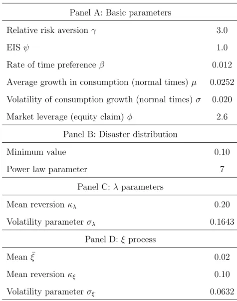
Table 1: Parameter values for the model
Panel A: Basic parameters
Relative risk aversion γ 3.0
EISψ 1.0
Rate of time preferenceβ 0.012
Average growth in consumption (normal times)µ 0.0252 Volatility of consumption growth (normal times)σ 0.020
Market leverage (equity claim)φ 2.6
Panel B: Disaster distribution
Minimum value 0.10
Power law parameter 7
Panel C: λ parameters Mean reversionκλ 0.20 Volatility parameterσλ 0.1643 Panel D:ξ process Mean ¯ξ 0.02 Mean reversionκξ 0.10 Volatility parameterσξ 0.0632
Notes: Panel A shows parameters for normal-times consumption and dividend processes, and for the preferences of the representative agent. Panel B shows parameters for the power law distribution that governs the tail of the consumption distribution. Panels C and D show the parameter values for λ and ξ processes:
dλt = κλ(ξt−λt)dt+σλ p λtdBλ,t+Zλ,tNλ,t dξt = κξ( ¯ξ−ξt)dt+σξ p ξtdBξ,t
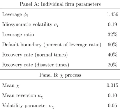
Table 2: Parameter values for an individual firm
Panel A: Individual firm parameters
Leverage φi 1.456
Idiosyncratic volatility σi 0.19
Leverage ratio 32%
Default boundary (percent of leverage ratio) 60%
Recovery rate (normal times) 40%
Recovery rate (disaster times) 20%
Panel B: χ process
Mean ¯χ 0.015
Mean reversion κχ 0.10
Volatility parameter σχ 0.05
Notes: This table reports the parameters for the total payout process on an individual firm. The default boundary in the model is computed as the leverage ratio (0.32) multiplied by 60%. Panel B shows parameter values for the χt process, where χt is the intensity of
idiosyncratic jumps. The process is given by
dχt = κχ( ¯χ−χt)dt+σχ √
χtdBχ,t+Zχ,tNλ,t.