K-CLASSES OF QUIVER CYCLES, GROTHENDIECK POLYNOMIALS, AND ITERATED RESIDUES
Justin Allman
A dissertation submitted to the faculty at the University of North Carolina at Chapel Hill in partial fulfillment of the requirements for the degree of Doctor of Philosophy in the Department of
Mathematics.
Chapel Hill 2014
c 2014 Justin Allman
ABSTRACT
Justin Allman: K-classes of quiver cycles, Grothendieck polynomials, and iterated residues
(Under the direction of Rich´ard Rim´anyi)
In the case of Dynkin quivers we establish a formula for the Grothendieck class of a quiver cycle as the iterated residue of a certain rational function, for which we provide an explicit combinatorial construction. Moreover, we utilize a new definition of the double stable Grothendieck polynomials due to Rim´anyi and Szenes in terms of iterated residues to exhibit that the computation of quiver coefficients can be reduced to computing the coefficients in a combinatorially prescribed Laurent expansion of the aforementioned rational function.
ACKNOWLEDGMENTS
The author is grateful to his advisor, Rich´ard Rim´anyi, for his guidance, support, and imparting his mathematical tastes. The author also thanks Anders Buch, Alex Fink, Ryan Kaliszewski, and Andr´as Szenes for helpful conversations related to these topics and Merrick Brown for computational advice, without which many lemmas, propositions, and theorems would never have been born as conjectures. The author thanks Michael Abel for conversations on this and other topics mathematical and otherwise.
TABLE OF CONTENTS
LIST OF SYMBOLS . . . viii
CHAPTER 1: INTRODUCTION . . . 1
1.1 Motivation from quiver loci . . . 1
1.1.1 Quiver representations . . . 1
1.1.2 Quiver cycles and Dynkin quivers . . . 2
1.2 Iterated residue operations. . . 5
CHAPTER 2: GROTHENDIECK POLYNOMIALS . . . 8
2.1 Combinatorial definition . . . 8
2.1.1 Stable Grothendieck polynomials . . . 8
2.1.2 Stable Grothendieck polynomials for general integer sequences . . . 9
2.1.3 The bialgebra structure . . . 12
2.1.4 Grothendieck polynomials in K-theory . . . 16
2.2 Grothendieck polynomials as iterated residues . . . 18
2.2.1 Definition and examples . . . 19
2.2.2 Encoding the bialgebra structure in iterated residue operations . . . 22
CHAPTER 3: THE CALCULUS OF ITERATED RESIDUE OPERATIONS. . . 25
3.1 Complete homogeneous symmetric functions and Schur functions . . . 25
3.1.1 Definitions and new iterated residue operations . . . 25
3.1.2 The anti-symmetrization operator . . . 27
3.2 Relating the iterated residue operations . . . 29
3.2.1 Expansions of Grothendieck polynomials as complete homogeneous symmetric functions . . . 29
CHAPTER 4: ON A CONJECTURE REGARDING ALGEBRAIC GENERATORS
FOR THE RING OF STABLE GROTHENDIECK POLYNOMIALS . . . 34
4.1 Partitions of length two . . . 34
4.2 Partitions of length exceeding two . . . 35
CHAPTER 5: DEGENERACY LOCI OF QUIVERS . . . 39
5.1 Quivers and degeneracy loci of vector bundles . . . 39
5.1.1 Quiver cycles for Dynkin quivers . . . 39
5.1.2 Degeneracy loci associated to quivers . . . 40
5.2 Resolution of singularities . . . 41
5.3 Main theorem . . . 44
5.4 On expansions of quiver polynomials in Grothendieck polynomials . . . 48
5.4.1 Examples . . . 49
APPENDIX A: EQUIVARIANT LOCALIZATION AND ITERATED RESIDUES . . . 54
APPENDIX B: PROOF OF THE MAIN THEOREM . . . 58
APPENDIX C: COMPUTATIONAL LEMMAS FOR ITERATED RESIDUE OPERATIONS . . . 62
LIST OF SYMBOLS
C,Z,N the complex numbers, integers, and natural numbers respectively ASymn the anti-symmetrization operator onnvariables
Gλ, sλ the stable Grothendieck, respectively Schur, polynomial for the partitionλ
t an alphabet of ordered commuting variables (t1, t2, . . .)
Grk(Cn) Grassmannian ofk-dimensional subspaces in Cn R[t] ring of polynomials int with coefficients inR
R[[t]] ring of formal power series int with coefficients inR R(t) ring of rational functions in t with coefficients inR R((t)) ring of formal Laurent series int with coefficients inR Λ the ring (Hopf algebra) of symmetric functions
Γ the bialgebra of stable Grothendieck polynomials E∨ the dual of the vector bundleE
Pn complex projectiven-space
hd complete homogeneous symmetric function of degreed ed elementary symmetric function of degreed
♦ denotes the end of a numbered remark or example
denotes the end of a proof or cited numbered theorem Σn the symmetric group onnletters
∆n(t) the discriminantQ1≤i<j≤n(ti−tj)
HG∗(X) G-equivariant cohomology (with integer coefficients) ofX KG(X) G-equivariant K-theory (with integer coefficients) ofX
Res
CHAPTER 1: INTRODUCTION
In this chapter we introduce several fundamental objects of study and fix notation. Much of the material presented below is an amalgam of definitions, examples, and exposition from the recent paper [All13].
1.1 Motivation from quiver loci
1.1.1 Quiver representations
The study of quivers has become ubiquitous in many branches of mathematics including algebraic geometry, algebraic combinatorics, representation theory, Lie theory, and the study of both commutative and non-commutative rings through the structure of cluster algebras.
A quiver Qis an oriented graph with a set of verticesQ0, and a setQ1 of oriented edges called
arrows (hence the name quiver). To every a∈Q1 we associate a head h(a) and tail t(a) in Q0.
Below is a quiver with three vertices and four arrows,
1 a2 2 3
a1
a3
a4
with Q0={1,2,3}and Q1 ={a1, a2, a3, a4} and e.g. h(a2) = 2,t(a4) = 3 and h(a1) =t(a1) = 1.
There is a natural geometric question associated to every quiver, which we now explain. Given a quiver Q= (Q0, Q1) with finite sets of vertices and arrows, label the verticesQ0 ={1, . . . , N}.
Now choose adimension vector v= (v1, . . . , vN) of non-negative integers. From this data, construct
vector spacesEi =Cvi and form therepresentation space
(1.1) V = M
a∈Q1
Hom(Et(a), Eh(a)).
quiver. This is separate from the fact thatV itself naturally carries an action of the algebraic group G=GL(E1)× · · · ×GL(EN). Explicitly, this is given by
(1.2) (gi)i∈Q0·(φa)a∈Q1 = (gh(a)φag
−1
t(a))a∈Q1
and one asks
Question 1.1. What are theG-orbits inV?
We conclude this subsection with two examples illustrating how answers to Question 1.1 are natural generalizations of fundamental concepts in linear algebra.
Example 1.2. LetE1andE2be vector spaces of respective dimensionse1ande2and letf :E1→E2
be a linear mapping. Up to changing bases in the source and target, there is only one invariant of the map f, namely its rank.
This situation corresponds to the quiver{◦ → ◦}, the dimension vector (e1, e2), the representation
space V = Hom(E1, E2), and the groupG= GL(E1)×GL(E2) where G acts on V by changing bases in the source and target. Notice that for any f ∈V (really just an e1×e2 matrix) there is
always an element ofGwhich can bring f to its reduced row-echelon form, from which the rank is
immediately readable. ♦
Example 1.3. Let n be a non-negative integer and consider the space ofn×n square matrices Matn(C). Up to similarity, an element of Matn(C) is determined by itsJordan normal form. This situation corresponds to the quiver with one vertex and a single loop arrow, with dimension vector (n), representation space V = Hom(Cn,Cn) = Matn(C), andG=GL(n,C) where Gacts on V by
conjugation. ♦
Note that for a fixed dimension vector Example 1.2 admits only finitely manyG-orbits while Example1.3 admits an infinite number. The quivers for which there are only finitely many orbits are exactly the Dynkin quivers, which we now define.
1.1.2 Quiver cycles and Dynkin quivers
Dynkin diagram (i.e. of typeAn,Dn,E6,E7, or E8) the quiver cycles are exactly G-orbit closures, of which there are only finitely many for each dimension vector [Gab72]. In this case, the quiver is called aDynkin quiver.
For such quivers, a major accomplishment of this dissertation project is a new calculation of the class
(1.3) [OΩ]∈KG(V),
in theG-equivariant Grothendieck ring ofV. En route, we reformulate the problem in an equivalent setting; we realize [OΩ] as the K-class associated to a certain degeneracy locus of a quiver of vector
bundles over a smooth complex projective base varietyX.
Formulas for this class exist already in the literature, the most general of which is due to Buch [Buc08], and which we now explain. Buch’s result is given in terms of the stable version of Grothendieck polynomials first invented by Lascoux and Sch¨utzenberger as representatives of structure sheaves of Schubert varieties in a flag manifold [LS82] which are applied to theEi in an appropriate way. For details specific to this context see [Buc08, Section 3.2], and for a comprehensive introduction to the role of stable Grothendieck polynomials in K-theory we refer the reader to [Buc05].
The stable Grothendieck polynomials Gλ are indexed by partitions, i.e. non-increasing sequences of non-negative integersλ= (λ1 ≥λ2 ≥ · · ·) with only finitely many parts nonzero. The number
of nonzero parts is called the length of the partition and denoted `(λ). For eachi∈Q0 define the
multiset of quiver vertices T(i) by forming the set
(1.4) T∗(i) ={(j, a)∈Q0×Q1|h(a) =iand t(a) =j}
and forgetting the second factors. In words, T(i) is a list of quiver vertices which admit arrows pointinginto icounted with multiplicities of arrows. Now form the vector spaceMi=L
j∈T(i)Ej.
With this notation, Buch shows that for unique integers cµ(Ω)∈Zone has
(1.5) [OΩ] =X
µ
where the sum is taken over all sequences of partitions µ= (µ1, . . . , µN) subject to the constraint that `(µi)≤vi for all 1≤i≤N. The integerscµ(Ω) are called thequiver coefficients. In the case that Q is a Dynkin quiver, that is, its underlying non-oriented graph is one of the simply-laced Dynkin diagrams (of type A, D, or E), Buch shows that the sum above is finite. The central question in the theory is
Question 1.4. Are the quiver coefficients alternating?
In this setting, alternating is interpreted to mean that for all µ,
(1.6) (−1)|µ|−codim(Ω)c
µ(Ω)≥0,
where |µ|=P
i|µi|and |µi| is the area of the corresponding Young diagram. An answer to this question supersedes many of the other positivity conjectures in this vein, in particular, whether or not the cohomology class [Ω] ∈ HG∗(V) is Schur positive, since the leading term of Gλ is the Schur functionsλ and the coholomology class [Ω] can be interpreted as a certain leading term of the K-class [OΩ]. For this reason, the quiver coefficients cµ(Ω) for which |µ|= codim(Ω) are called the cohomological quiver coefficients.
The seminal paper by Buch and Fulton [BF99] on quiver loci fixed much of the original interest on theequioriented typeAproblem (i.e. all the arrows point in the same direction). In the cohomological setting, there are many affirmative results on Schur positivity in this case, see for example [BFR05], [KS06], and [KMS06]. In the alternative basis of Schubert polynomials for type Athere are positive formulae presented in [BKTY04] and [BR07] in the equioriented and non-equioriented settings respectively. Using an entirely independent approach Feh´er and Rim´anyi [FR02] have related the theory of Thom polynomials for group actions directly to quivers and bring to bear the restriction method of Rim´anyi. This was the first paper to consider the general Dynkin case.
The progress for general Dynkin quivers is more sparse, but Buch [Buc08] has proven the K-theoretic quiver coefficients alternate (and hence that the cohomological quiver coefficients are
positive) in the case ofA3 quivers with arbitrary arrows and dimension vectors. Kaliszewski has
shown Schur positivity in cohomology for some special cases of non-equioriented A4 quivers. To the
residue operations. The motivation is plain—namely there has been some considerable recent success
in attacking positivity and stability results in analogous settings once armed with such a formula. In [FR07], Feh´er and Rim´anyi discover that Thom polynomials of singularities share unexpected stability properties, and this is made evident through non-conventional generating sequences. The ideas of [FR07] are further developed and organized in [BS12], [FR12], and [Kaz10b] where the generating sequence formulas appear under the name iterated residue. In particular, in [BS12] B´erczi and Szenes prove new positivity results for certain Thom polynomials, and Kazarian is able to calculate new classes of Thom polynomials in [Kaz10b] through iterated residue machinery developed in [Kaz10a].
Even more recently, a new formula for the cohomology class of the quiver cycle in H∗ G(V) as an iterated residue has been reported in [Rim14], and Kaliszewski’s positive results for certain non-equiorientedA4 quivers [Kal13] were obtained from this formula. Moreover in [Rim13], Rim´anyi
describes an explicit connection between the iterated residue formula for cohomological quiver coefficients of [Rim14] and certain structure constants in the cohomological Hall algebra (CoHa) of Kontsevich and Soibelman [KS11].
1.2 Iterated residue operations
Letf(x) be a rational function in the variable x with coefficients in some commutative ringA which has a formal Laurent series expansion in A((x)). Define the operation
(1.7) Res
x=0,∞(f(x)dx) = Resx=0(f(x)dx) + Resx=∞(f(x)dx),
where Resx=0(f(x)dx) is the usual residue operation from complex analysis (i.e. take the
coeffi-cient of x−1 in the corresponding Laurent series about x = 0), and furthermore one recalls that Resx=∞(f(x)dx) = Resx=0(df(x1)). The idea of using the operation Resx=0,∞in K-theory is due to Rim´anyi and Szenes [RS14].
series expansion inA((z1, . . . , zn)). Then one defines
Res
z=0,∞(F(z)dz) =znRes=0,∞
· · · Res z1=0,∞
(F(z)dz1· · ·dzn).
Later, in Section2.2we will also make use of the shorthand notation dlog(z) to mean the product
Q
id(log(zi)) =
Q
i dzi
zi .
Example 1.5. Consider the functiong(x) = (1−x/y1 )x. Using the convention thatx << y (which we use throughout the sequel), we obtain that
Res
x=0(g(x)dx) = Resx=0
1 x
1 +x y +
x2 y2 +· · ·
dx
= 1.
On the other hand,
−1
x2g(1/x) =y
1 1−xy
and so Resx=∞(g(x)dx) = 0. Thus Resx=0,∞(g(x)dx) = 1. However, it is more convenient to do
the calculation by using the fact that for any meromorphic differential form the sum of all residues (including the point at infinity) is zero. Since the only other pole ofg occurs at x=y, we see easily
that
Res
x=0,∞(g(x)dx) =−Resx=y
dx (1−x/y)x
= 1,
just as we calculated beforehand. ♦
Example 1.6. Consider the meromorphic differential form
F(z1, z2) =
(1−β1
z2)(1−
β2
z2)(1−
z2
z1)
(1− z1
α1)(1−
z2
α1)(1−
z1
α2)(1−
z2
α2)z1z2
dz1dz2.
Functions of this type will occur often in our analysis, where the result of the operation Resz=0,∞(F)
is a certain (Laurent) polynomial in the variables αi and βj, separately symmetric in each. We begin by factoringF =F1F2, where
F1 =
(1−z2
z1)
(1− z1
α1)(1−
z1
α2)z1
dz1 and F2=
(1−β1
z2)(1−
β2
z2)
(1− z2
α1)(1−
z2
α2)z2
We first use the residue theorem as in the previous example to write that
Res z1=0,∞
(F) =−
Res z1=α1
(F) + Res z1=α2
(F)
,
and we compute that
− Res z1=α1
(F) =−F2
Res z1=α1
(F1)
=F2
(1− z2
α1)
(1−α1
α2)
!
=F0
− Res z1=α2
(F) =−F2
Res z1=α2
(F1)
=F2
(1− z2
α2)
(1−α2
α1)
!
=F00
It is not difficult to see that Resz2=α1(F
0) = Resz
2=α2(F
00) = 0, so it remains only to compute
Res
z=0,∞(F) =−zRes2=α2
(F0)− Res z2=α1
(F00)
= (1− β1
α2)(1−
β2
α2)
(1−α1
α2)
+(1− β1
α1)(1−
β2
α1)
(1−α2
α1)
= 1− β1β2 α1α2
.
The last line above bears resemblance to a Berline-Vergne-Atiyah-Bott type formula for equivariant localization, adapted for K-theory. This is not accidental, a connection which we explain in Section
CHAPTER 2: GROTHENDIECK POLYNOMIALS
2.1 Combinatorial definition
Most of the original work on the combinatorial treatment of the stable Grothendieck polynomials can be found in the papers [Buc02b], [Buc02a], [Buc05], and [Buc08]. Below we fix our notation for these polynomials and list several important properties.
2.1.1 Stable Grothendieck polynomials
A partition λ = (λ1 ≥ λ2 ≥ . . . ≥ λN ≥ 0) is a weakly decreasing sequence of non-negative integers. The length `(λ) is the number of nonzero parts, and theweight |λ|is the sum of the parts
PN
i=1λi. Given two partitionsλandµ, we say that λcontains µand writeµ⊂λifµi≤λi for each
i≥1. Every partition can be identified with itsYoung diagram of boxes; explicitly, the diagram associated to λis the left justified array of boxes with λ1 boxes in the first row, λ2 boxes in the
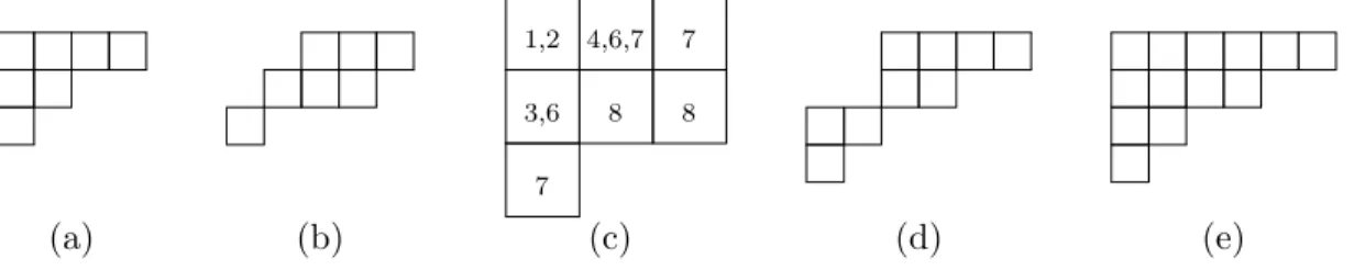
second, and so on. Hence, the area of the Young diagram is exactly|λ|and the height is exactly `(λ). For example, the partition (4,2,1) is associated to the diagram in Figure2.1(a). A skew shape is given by a pair of partitionsµ⊂λand denotedλ/µ. The associatedskew diagram is obtained by removing the shape µfrom the upper left-hand corner of the diagram for λ; e.g. the diagram in Figure 2.1(b) is the skew Young diagram (5,4,1)/(2,1).
A set valued tableau T is a filling of the boxes of any (skew) Young diagram by sets of positive integers subject to the following rules: (a) the content of each box is a non-empty, finite, strictly increasing sequence of positive integers, (b) the filling must weakly increase reading left to right
1,2 4,6,7 7
3,6 8 8 7
(a) (b) (c) (d) (e)
along rows, and (c) the filling must strongly increase down columns.
Given a filling T and a set x = (x1, x2, . . .) of commuting variables, we define xT to be the
monomial in which the exponent ofxi is the number of boxes ofT in which the integeriis contained. We write sh(T) to denote its shape and |T|to denote the degree of the monomial xT. For example, the set valued tableau in Figure2.1(c) has sh(T) = (3,3,1),xT =x1x2x3x4x26x37x28, and|T|= 11.
The single stable Grothendieck polynomial for any partitionλin the variables x= (x1, x2, . . .)
can be defined to be [Buc02b, Theorem 3.1]
(2.1) Gλ(x) =Gλ(x1, x2, . . .) := X
sh(T)=λ
(−1)|T|−|λ|xT.
Of course, this expression is actually a formal power series, but often in applications, only finitely many of the variables xi are nonzero, and equation (2.1) in fact represents a polynomial. In particular, throughout the sequel, whenever we write Gλ(x1, . . . , xm) we mean the expression Gλ(x1, . . . , xm,0,0, . . .). It is known that the series (2.1) is symmetric. It is non-homogeneous, but notice that the lowest degree term corresponds to fillings with |T| = |λ|, when T is just a semi-standard Young tableau. It follows that the lowest degree term of the series is the well-known Schur function sλ(x).
Often we will write simply Gλ forGλ(x1, x2, . . .) when either the number of variables present is
clear from the context, or when the formula we are writing is true independently of the number of variables. In all that follows, we set Γ =L
λZGλ where the sum is taken over all partitionsλ.
2.1.2 Stable Grothendieck polynomials for general integer sequences
In many of our formulas, we will need to deal with integer sequences I ∈ Zn which are not partitions. In particular, we wish to define stable Grothendieck polynomialsGI(x) for such sequences. In this section, we follow Buch’s formulation from [Buc02a].
or more elegantly, the coefficient ofqk in the expansion of
1
Qm
j=1(1−xjq)
.
Now, we wish to generalize these polynomials to the non-homogeneous case. Let h(ki)(x1, . . . , xm)
denote the coefficient of qk in the power series expansion of
(2.2) (1−q)
i
Qm
j=1(1−xjq) .
Note in particular that h(0)k (x1, . . . , xm) = hk(x1, . . . , xm), and that for any i ∈ Z, one has the identities h(0i)(x1, . . . , xm) = 1 while h(ki)(x1, . . . , xm) = 0 for k <0.
Now, we define
(2.3) gI(x1, . . . , xm) := (−1)m(m−1)/2det
h(Ii−1)
i+j−1(x1, . . . , xm)
1≤i,j≤m.
Notice that the size of the determinant depends on m, the number of x-variables, and so by convention, we agree that λi = 0 for i > n. Notice this implies that g∅(x1, . . . , xm) = 1. The
importance of these determinants for our purpose is given by:
Proposition 2.1 (Lenart [Len00]). Wheneverλ= (λ1, . . . , λn) is a partition and m≥n,
(2.4) Gλ(x1, . . . , xm) =gλ(x1, . . . , xm).
The determinant in Equation (2.3) can be manipulated to show that the polynomials gI satisfy a certain recursive relation (independent of the number of variables), which can be used to transform gI(x1, . . . , xm) uniquely into aZ-linear combination of polynomialsgλ(x1, . . . , xm) withλa partition. Proposition 2.2 (Buch [Buc02a]). Let m be a positive integer.
(a) Suppose that J and K are any integer sequences and p < q are integers. Then
(2.5) gJ,p,q,K(x1, . . . , xm) = q
X
r=p+1
gJ,q,r,K(x1, . . . , xm)− q−1 X
s=p+1
(b) Let I = (I1, . . . , In) be a sequence of integers such that m≥n and m≥i−Ii, for all 1≤i≤n. ThengI(x1, . . . , xm) is a finite linear combination of determinants gλ(x1, . . . , xm) for partitions
λ:
(2.6) gI(x1, . . . , xm) =
X
λ
δI,λgλ(x1, . . . , xm).
Furthermore, the coefficients δI,λ∈Z are independent ofm.
In the latter summation of part (a), if the condition p+ 1≤s≤q−1 cannot be met, (i.e. if q =p+ 1) the sum is considered to be zero. The results of the previous two propositions imply that it is natural to define for any integer sequence I and any collection of commuting variables
x= (x1, x2, . . .) that
(2.7) GI(x) :=
X
λ
δI,λGλ(x).
The result of Proposition 2.2(b) implies that this is a well defined element of Γ. Further, since GI(x1, . . . , xm) = gI(x1, . . . , xm) when m is sufficiently large, we obtain that GI(x) =
limm→∞gI(x1, . . . , xm). Notice also that for p < q, we obtain
(2.8) GJ,p,q,K =
q
X
r=p+1
GJ,q,r,K − q−1 X
s=p+1
GJ,q−1,s,K
by Proposition 2.2(a). This can be written more succinctly as the recursion
(2.9) GJ,p,q,K =GJ,q,p+1,K−GJ,q−1,p+1,K+GJ,p+1,q,K.
Moreover, wheneverJ is a sequence consisting only of nonpositive integers,GI,J =GI. These facts have the consequence that GI isnever zero forany integer sequence I, which is quite different from the case of (fake) Schur functionssI. Indeed, recall that for any integer sequenceI = (I1, . . . , In) one can define a fake Schur function sI by extending the Jacoby-Trudi formula [Mac95, Equation I.3.4] to take in non-partition integer sequences. In particular, one defines for I = (I1, . . . , In),
(2.10) sI := det (hIi+j−i)
where hddenotes the complete homogeneous symmetric function of degree d. This is equal either to zero or ±sλ for some partition λof length no more thannand moreover has the property that |λ|=|I|. The leading term of Gλ issλ, and observe that the recursive process defined by equation (2.8) is consistent with the analogous process for changingsI into±sλ (in the latter case, simply interchange rows in the determinant above). In particular, equation (2.8) can produce no more than one termGλ such that|λ|=|I|.
Example 2.3. Observe that
G−2,1 =G1,−1+G1,0+G1,1−G0,−1−G0,0 = 2G1+G1,1−2G∅ = 2G1+G1,1−2
by noting thatG∅ = 1∈Γ (cf. Section2.1.3). On the other hands−2,1= 0. ♦ Remark 2.4. For λ= (λ1, . . . , λN) and x = (x1, . . . , xN), the determinant in equation (2.3) is equivalent to the polynomial defined by
Gλ(q :x) = 1 ∆N(x)det
xλi+N−i
j (1 +qxj)i−1
1≤i,j≤N
with q = −1 where ∆N(x) is the discriminant. This is true, say, by the method of [Len00, Theorem 2.4]. The author is aware that the physicists use this formula, see for example [MS13], and in this light one views the Grothendieck polynomialGλ as a one parameter deformation of sλ by comparing the formula above with the definition of Schur functions by a similar expression as in [Mac95, Equation I.3.1]. To wit
sλ(x1, . . . , xN) = 1 ∆N(x)
detxλi+N−i j
1≤i,j≤N
is the classical limit ofGλ(q:x) withq →0. ♦
2.1.3 The bialgebra structure
Consider the Z-linear span Γ = L
To every set valued tableau T we associate its word w(T), which is the sequence of integers obtained by ordering the rows from bottom to top and reading off the entries of each row from left to right. Thecontent of a word is the sequenceγ = (γ1, γ2, . . . , γN) whereγi is the number of
times iappears in the word. Notice that the monomialxT is the monomialxγ=xγ1
1 x
γ2
2 · · ·x
γN N . A word is called a reverse lattice word if every appearance of an integer i≥2 is followed by strictly more occurrences ofi−1 thani. For example, the set valued tableau shown in Figure2.1(c) has w(T) = (7,3,6,8,8,1,2,4,6,7,7) with content γ = (1,1,1,1,0,2,3,2). It fails to be a reverse lattice word since the leading 7 is followed by two 6’s but also two 7’s.
Given two partitions λ and µwe define the diagram λ∗µ to be the skew shape obtained by attaching the bottom left corner of µ to the top right corner of λ. Equivalently, if one defines the diagram R to be the rectangle with height `(µ) and widthλ1, the diagramλ∗µis the skew
diagram (R+µ, λ)/R. For example (2,1)∗(4,2) produces the diagram in Figure2.1(d). Finally, given partitionsλ,µ, and ν we can define the integerscνλµ and dνλµ.
Let cνλµ be (−1)|λ|+|µ|−|ν| times the number of set valued tableaux T of shape λ∗µ, subject to the constraint that w(T) is a reverse lattice word of content ν. Then set dν
λµ =c ρ
νR whereR is a rectangular partition with length at least `(µ) and width at least λ1, andρ is the partition
(R+µ, λ). It is an exercise to show this definition is independent ofR (cf. [Buc05]). For example, with λ= (2,1) and µ= (4,2), one takes R= (2,2) andρ is represented by the diagram in Figure
2.1(e). The meaning of these integers is given by the following two theorems, both due to Buch [Buc02b].
Theorem 2.5. The product of two stable Grothendieck polynomials is given by the formula
(2.11) Gλ·Gµ=
X
ν
cνλµGν
where the sum is taken over all partitions ν.
as the unit in Γ.
Theorem 2.6. For any integers 0< j < m,
Gν(x1, . . . , xm) = X
λ,µ
dνλµGλ(x1, . . . , xj)Gµ(xj+1, . . . , xm)
where the sum is over all pairs of partitions λand µ.
This defines a coassociative and cocommutative coalgebra structure on Γ with coproduct ∆ : Γ−→Γ⊗Γ given by
(2.12) ∆(Gν) =
X
λ,µ
dνλµGλ⊗Gµ.
The counit map ε: Γ→Zis given byε(Gλ) =δ∅,λ for every partitionλwhere δij is the Kronecker delta function.
Example 2.7. Since the integers dνλµ are themselves multiplicative structure constants in Γ, one can compute the comultiplication from the multiplication as follows. In order to compute ∆(Gν), choose a rectangle R containing ν and consider the product GνGR=PτcτνRGτ. It is not difficult to observe that for each τ in the expansion the skew diagram τ /Rhas the form λ∗µfor someλ and µand so cτνR=dνλµ. For example (cf. [Buc05, Example 5]),
G ·G =G +G +G +G +G +G
−2G −G −G −G −G −2G
and therefore one obtains the expansion
∆G = 1⊗G +G ⊗G +G ⊗G +G ⊗G +G ⊗G +G ⊗G
=−2G ⊗G −G ⊗G −G ⊗G +G ⊗G −G ⊗G −2G ⊗G
+G ⊗G +G ⊗G +G ⊗G +G ⊗G −G ⊗G
for the comultiplication. ♦
Now let y= (y1, y2, . . .) be an additional set of commuting variables, and define also thedouble
stable Grothendieck polynomial to be
(2.13) Gν(x;y) :=
X
λ,µ
dνλµGλ(x)Gµ0(y)
where the Grothendieck polynomials on righthand side are single stable Grothendieck polynomials inxandy, andµ0 denotes the conjugate (or transpose) of the partitionµ(i.e. the rows and columns are exchanged in the Young diagram). Moreover, just as in Equation (2.7), one defines
(2.14) GI(x;y) :=X
λ
δI,λGλ(x;y).
These polynomials are separately symmetric in xand y, and moreover satisfy the identities
(2.15) Gν(1−a−1,x; 1−a,y) =Gν(x;y)
for any indeterminate a, and if z and ware still two more sets of commuting variables,
(2.16) Gν(x,z;y,w) =
X
λ,µ
dνλµGλ(x,z)Gµ0(y,w)
and moreover
(2.17) Gν(x,z;y,w) =
X
λ,µ
dνλµGλ(x;y)Gµ(z;w).
one alphabet with z appended to x, while (x;y) are considered as two separate alphabets as in equation (2.13). In the literature, sometimes these are denoted by x+zand x−y respectively.
In the case that y= 0, Gλ(x;y) =Gλ(x), the single stable Grothendieck polynomial. Two more helpful relations are given by
Gλ(x1, . . . , xn) = 0 whenever `(λ)> n (2.18)
Gµ(x;y) =Gµ0(y;x) (2.19)
for any partitionµand alphabetsxandy. The first relation is readily checked from Buch’s theorem expressing Gλ(x) in terms of set-valued tableaux, cf. Equation (2.1), while the second is originally attributed to Fomin (see [Buc02b, Lemma 3.4] for an interesting anecdote). Note the latter implies that ifx= 0 thenGλ(x;y) =Gλ0(y).
2.1.4 Grothendieck polynomials in K-theory
Now suppose thatXis a smooth complex projective variety, and letK(X) denote the Grothendieck ring of isomorphism classes of algebraic vector bundles overX. If E −→X is a vector bundle which splits as a sum of line bundles, say E=Ln
r=1Er, then for a partitionλone defines,
(2.20) Gλ(E) :=Gλ(1−[E1]−1, . . . ,1−[En]−1),
where the righthand side is the single stable Grothendieck polynomial of equation (2.1) evaluated on the variables xi = 1−[Ei]−1 for 1≤i≤nand xj = 0 otherwise. Since Gλ is symmetric, the righthand side above is actually a polynomial in the classes of exterior powers of the dual vector bundleE∨, and henceG
λ(E) is a well defined class inK(X) forany vector bundle E. IfE0 −→X is any other vector bundle, one defines for any partition ν
Gν(E0+E) = X λ,µ
dνλ,µGλ(E0)Gµ(E) (2.21)
Gν(E0− E) = X λ,µ
Notice that since every element of K(X) can be realized as a Z-linear combination of classes of vector bundles, the identities of equations (2.15), (2.16), (2.17), combined with the results of Section
2.1.2imply that GI(F) is made into a well-defined element of K(X) forany integer sequenceI and any classF ∈K(X). Moreover, for vector bundles E and F, the relations of Equations (2.18) and (2.19) translate respectively to this setting as
Gλ(E) = 0 whenever `(λ) exceeds the rank ofE (2.23)
Gµ(E − F) =Gµ0(F∨− E∨). (2.24)
for any partitionµand arbitrary ranks for E and F.
Remark 2.8. The multiplication and comultiplication of Grothendieck polynomials have geometric interpretations as follows.
Let X= Grk(Cn) denote the Grassmannian ofk-planes in Cn over which lies the tautological exact sequence of vector bundles 0→ S →Cn→ Q →0. Recall that to each partition λcontained in the rectangular partition (n−k)k corresponds a Schubert variety Xλ. The classes [OXλ] of the structure sheaves of Schubert varieties form an additive basis of the ringK(X) and moreover, [OXλ] =Gλ(S∨). The ringK(X) is thus identified with the quotient of Γ by partitions not fitting inside the rectangle (n−k)k. Thus, analogous to the case of cohomology and the product of Schur functions, the productGλ·Gµ=PνcνλµGν provides information regarding the intersection of the two Schubert varieties [Xλ] and [Xµ] once placed in general position. For more details see Buch’s introductory exposition in [Buc02b]. In fact the higher order terms, i.e. those corresponding toGν with |ν| |λ|+|µ|, have an interpretation in light of Vakil’s degeneration techniques (cf. [Vak06] and [Buc05, Example 2]) for computing products in the cohomology ring H∗(X).
As for the comultiplication, consider the mapping
ψ: Grk1(n1)×Grk2(n2)→Grk1+k2(n1+n2)
sending (V1 ⊂Cn1, V
2 ⊂Cn2)7→V
1⊕V2 ⊂Cn1+n2. Letting S
subbundles over Grk1(n1), Grk2(n2), and Grk1+k2(n1+n2) we write that
ψ∗Gν(S) =Gν(ψ∗S) =Gν(S1⊕S2) = X
λ,µ
dνλ,µGλ(S1)·Gµ(S2).
Note that in order to writeS1⊕S2 above, we have identifiedS1 andS2 with pullbacks. This implies
that the comultiplication corresponds to the pullback mapping along the embeddingψ. ♦
Remark 2.9. It is known that the ring of symmetric functions admits a commutative, cocommutative Hopf algebra structure with antipodeS : Λ→Λ obtained from the involution sλ 7→sλ0 (with a sign correction). For more details regarding the natural Hopf algebra structure on Λ begin with [Mac95, Example I.5.25] and see also [Sta99, Section 7.15] and [Zel81, Section 5].
In contrast, the bialgebra Γ cannot be made into a Hopf algebra (see [Buc02b, Section 9]) even though it is a subalgebra of Λ. Indeed, if so the antipodeS must satisfy (cf. [All09, 2.2.2(i)])
0 =S(G1) + 1−S(G1)G1 = 1 +S(G1)(1−G1)
which implies that 1−G1 must be invertible in Γ. This is false, so no such antipode can exist.
However, according to Buch [Buc02b] the elementt= 1−G1 is formally invertible when multiplied
by the sum of all partitionsP
λGλ and when Γ is completed to allow infinite linear combinations of Grothendieck polynomials, this is enough to ensure it becomes a Hopf algebra. ♦
2.2 Grothendieck polynomials as iterated residues
In this section, we will explain a new formula for the stable Grothendieck polynomials in terms of iterated residue operations due to Rim´anyi and Szenes [RS14]. Throughout this section we always assume thatGλ(x;y) has only finitely many non-zero x andy variables. Moreover, we introduce new variablesαi and βj byxi = 1−αi−1 and yj = 1−βj and in this context, write simplyGλ(α;β) for the polynomial Gλ(x;y).
In particular, take A and B to be vector bundles over X of respective ranks n and m, and let α = {α1, . . . , αn} (respectively β = {β1, . . . , βm}) such that [VkA] = ek(α) (respectively [V`B] =
cohomology. Notice that if the variables αi are Grothendieck roots of A, then {α−11, . . . , α−n1} is a set of Grothendieck roots of A∨. Finally, following the recipe of Section 2.1.4 we see that Gλ(α;β) =Gλ(A − B)∈K(X).
2.2.1 Definition and examples
Letλbe a partition of lengthr,α={α1, . . . , αn}, β={β1, . . . , βm}and set `=n−m. Consider the alphabet of commuting variablesz={z1, . . . , zr} and form the products
Mλ(z) = r
Y
i=1
(1−zi)λi−i
P(z) = r
Y
i=1
(1−zi)`
Qm
j=1(1−ziβj)
Qn
k=1(1−ziαk) δ(z) = Y
1≤i<j≤r
1−zj zi
.
Define the polynomial
(2.25) gλ(α;β) = Res
z=0,∞(Mλ(z)P(z)δ(z)dlog(z)).
We reserve the right to use the word “polynomial” because although the result of applying Equation (2.25) is technically a Laurent polynomial in the variables α and β, upon passing to the x and y variables of Section 2.1 the expression indeed has only non-negative exponents. In [RS14] it is proven that whenever λis a partition, the polynomialgλ(α;β) agrees exactly with the double stable Grothendieck polynomialsGλ(α;β). Moreover, even whenλis not a partition, the polynomial gλ obeys the recursion of Equation (2.9) from whence it follows that
Theorem 2.10. GI(α;β) =gI(α;β) for any integer sequence I.
Remark 2.11. Henceforth, we will take the expression in Equation (2.25) as the definition of the double stable Grothendieck polynomialGI(α;β). The advantage is that whenever one sees an expression of the form
Res
z=0,∞(f(z)P(z)δ(z)dlog(z)),
infinite) of Grothendieck polynomials simply by reading off exponents of (1−zi) in each term. This
is the central idea of the rest of this thesis. ♦
We wish to introduce a new operation G•
• which we will use throughout the sequel. In some sense, it removes the unnecessary notation from Equation (2.25) and allows one to focus simply on the functionf of the above remark. The “bullets” represent optional decorations which we now describe.
For i ≥1, let ti = (ti1, ti2, . . .) be alphabets of ordered commuting variables. Given a finite
integer sequenceI = (I1, . . . , In) we use the standard multi-index notationtIi to denote the monomial
Qn
i=1t
Ij
ij. Letλi = (λi1, . . . , λini) be finite integer sequences (not necessarily partitions), and for everyN ≥1 define the following operations on monomials in the ringR =Z((ti))
Gt1,...,tN N
Y
i=1 tλi
i
!
= N
O
i=1
Gλi. (2.26)
Moreover, ifai is anything which can be “plugged into” a Grothendieck polynomial (e.g. collections– with or without semicolons–of commuting variables, formal Z-linear combinations of vector bundles over a smooth base, etc.), then we define
Ga1,...,aN
t1,...,tN N
Y
i=1 tλi
i
!
= N
Y
i=1
Gλi(ai). (2.27)
We will refer also to the G•
• operation as an iterated residue operation, but wait to justify this terminology until Section3.1. Extend these operations linearly to theZ-submoduleR0 ⊂Rfor which the result is a finite Z-linear combination of (tensor) products of stable Grothendieck polynomials. With these conventions, Equation (2.26) defines aZ-linear mapping
Gt1,...,tN :R0−→Γ⊗N
and e.g. if theai above represent classes inK(X) for a smooth baseX then Equation (2.27) defines a Z-linear mapping
Ga1,...,aN
t1,...,tN :R
We also allow G{ti} to act on rational functions in Z(ti) provided they have a formal Laurent expansion inR.
Remark 2.12. Depending on what objects are represented by theai, the submoduleR0 for which the operation Ga1,...,aN
t1,...,tN is defined may be strictly larger than the submodule on which the operation Gt1,...,tN is defined.
As an example, take only one alphabet t = (t1, t2, . . .) and consider the power series f(t) = P∞
k=0tk1. The result of applying the operation Gt is the infinite sum Pk≥0Gk, which is not an element of Γ. However, if one lets L −→X be a line bundle, then
Gt−L∨(f) = ∞
X
k=0
Gk(−L∨) = ∞
X
k=0
G(1)k(L) = 1 +G1(L)
which is a well-defined element of K(X). In the arithmetic above, we have used the relation on double stable Grothendieck polynomials thatGλ(x;y) =Gλ0(y;x) and on single stable Grothendieck polynomials thatGλ(x1, . . . , xn) = 0 whenever`(λ) exceedsn. We will not usually need such explicit
distinctions in the sequel. ♦
Example 2.13. Lett= (t1, t2, . . .) and consider the operation
(2.28) Gt t1t2
1−t1
1−t1
t2
!!
.
The rational function inside can be rewritten as
t1t2(1−t1) 1 +
t1
t2
1− t1
t2
!
=t1t2(1−t1) +t21
1−t1
1− t1
t2
where the second term has only non-positive powers of t2. By the relation thatGI,p =GI whenever p ≤ 0, the expression above is equivalent under the Gt operation to the function obtained by replacingt2 = 1 in the second term. Namely we need only applyGt to the polynomial
t1t2(1−t1) +t21=t1t2+t21−t21t2.
the operation
GtL t1t2
1−t1
1− t1
t2
!!
is equal to G2(L)∈K(X) since Gλ(x1, . . . , xN) = 0 whenever `(λ) exceedsN. ♦
In the next subsection, we will see that the G•• operation can efficiently encode much of the bialgebra structure of Γ, avoiding the difficult computational problem of counting set-valued tableaux.
2.2.2 Encoding the bialgebra structure in iterated residue operations
Suppose that we are given two arbitrary integer sequencesI and J of respective lengths n and m, and we form GI andGJ in Γ. We wish to compute the productGI·GJ on the level of iterated residues, namely using Equation (2.25). We form alphabets x= (x1, . . . , xn) andy= (y1, . . . , ym)
and choose α = (α1, . . . , αN) and β = (β1, . . . , βN) for some very largeN. In fact, it suffices to
choose any N ≥ n in order to see every non-zero term of GI ·GJ = P
νcνI,JGν in the product GI(α;β)·GJ(α;β). We then represent the product as the iterated residue
(2.29) GI(α;β)·GJ(α;β) = Res
x=0,∞yRes=0,∞(MI(x)MJ(y)P(x)P(y)δ(x)δ(y)).
Now form a new alphabetz defined byzi =xi for 1≤i≤nandzn+j =yj for 1≤j≤m. Under this transformation, notice that P(x)P(y) =P(z) and moreover
(2.30) δ(x)δ(y)
n Y i=1 m Y j=1
1−yj xi
=δ(z).
Notice that for everyiand j one has
1−yj xi =
1
xi ((1−yj)−(1−xi)) = 1−yj
xi
1−(1−xi) (1−yj)
.
Combining this observation with the identity of Equation (2.30), we obtain thatMI(x)MJ(y)δ(x)δ(y) equals
MI(x)MJ(y)
Qm
j=1(1−yj)n
!
Qn i=1xmi
Qn
i=1 Qm
j=1
1− (1−xi)
(1−yj)
δ(x)δ(y)
n Y i=1 m Y j=1
1−yj xi
which in the zvariables becomes the expression
(2.31) MI,J(z)
Qn
i=1zim
Qn
i=1 Qm
j=1
1− (1−zi)
(1−zn+j)
δ(z).
Finally, making the substitution zk = 1−tk for all k, we can prove that
Theorem 2.14. For integer sequences I andJ as above, one has
(2.32) GI·GJ =Gt
n
Y
i=1
tIi i
m
Y
j=1
tJj n+j
n
Y
i=1
(1−ti)m
Qm
j=1(1−tit
−1
n+j)
!
Proof. Indeed, Equation (2.25) implies that inserting the expression of (2.31) times P(z)dlog(z) into the operation Resz=0,∞ should yield the result. One needs only to expand the parenthetical part of (2.31) as a Laurent series about zk= 1 for each kto see the integer sequences appearing in the product GI·GJ =P
KaKI,JGK. Equivalently, one expands the rational function in equation (2.32) as a Laurent series abouttk = 0 for eachk.
Remark 2.15. It will occur often enough that we wish to give a name to the rational function
(2.33) Kn,m(t) =
n
Y
i=1
(1−ti)m
Qm
j=1(1−tit−n+1j)
which appears in equation (2.32). We will borrow terminology from the theory of partial differential equations and callKn,m themultiplication kernel. This natural moniker was suggested to the author
by Mihalcea. ♦
Example 2.16. The theorem implies that G1·G1 is equal to applying the Gt operation to the
rational function
t1t2
1−t1
1−t1t−21
,
which from Example 2.13we know is equal to G11+G2−G21. ♦
Corollary 2.17. For any integer sequence I of length n, the element ∆(GI)∈Γ⊗Γ is given by
(2.34) Gt,s tI
n
Y
i=1
(1−si)n
Qn
j=1(1−sit−j1)
!
Proof. Set m= max(I). If this number is non-positive, then GI =G∅ = 1∈Γ. In this case each variabletj occurs only with non-positive exponents. Hence the expression in (2.34) is equivalent under Gt,s to the one obtained by specializing tj = 1 for all j. Again becauseGI = 1, the result is the element 1⊗1∈Γ⊗Γ as desired.
If m >0 consider the rectangular partition R= (m)n. Then every partitionλappearing with nonzero coefficient in the expansionGI =P
λδI,λGλ of Equation (2.7) is contained inR. Theorem
2.14implies that we can encode the product GR·GI by applying Gu to the rational function
n
Y
i=1
umi n
Y
j=1
uIj
n+jKn,n(u).
As in Example 2.7we can obtain the comultiplication from this multiplication, and in the language of iterated residues, this corresponds to substituting si = ui for 1 ≤ i ≤ n and tj = un+j for 1≤j≤nabove anddividing the result by the monomial sR=Qn
i=1smi . The result is exactly the formula of Equation (2.34).
Remark 2.18. In analogy with our definition of a multiplication kernel, we define also a comulti-plication kernel
(2.35) Kˆn,m(t,s) =
m
Y
i=1
(1−si)n
Qn
j=1(1−sit−j1)
CHAPTER 3: THE CALCULUS OF ITERATED RESIDUE OPERATIONS
3.1 Complete homogeneous symmetric functions and Schur functions
3.1.1 Definitions and new iterated residue operations
Recall the definition of ti, λi, andR from Section 2.2.1 and used in Equation (2.26). Define anotheriterated residue operation S•
• in analogy with theG•• operation as follows
(3.1) St1,...,tN
N
Y
i=1 tλi
i
!
:= N
O
i=1
sλi
where sλi denotes the (possibly “fake”) Schur function, cf. Equation (2.10). The result of this operation is an element of the N-th tensor power of the ring of symmetric functions Λ. Moreover, if the symbols ai represent anything which can be “plugged into” a Schur function, then we can define also the operation
(3.2) Sa1,...,aN
t1,...,tN N
Y
i=1 tλi
i
!
:= N
Y
i=1
sλi(ai).
An important special case is when the ai represent formal differences of vector bundles over a
smooth baseX. Explicitly, for vector bundlesV andW over X define the relative Chern classes cn(V − W)∈H∗(X) by the formal expression
(3.3) X
n≥0
cn(V − W)ξn=
P
k≥0ck(V∨)(−ξ)k
P
`≥0c`(W∨)(−ξ)`
where ck(V∨) and c`(W∨) represent the Chern classes ofV∨ and W∨ inH∗(X) respectively. Then one defines
sλ(V − W) = det(cλi+j−i)
where ck is the relative Chern classck(V − W) defined above. In this case, Sai
Finally, in the special case that ai = xi = (xi1, . . . , xini) are finite collections of commuting variables, we can also define
(3.4) Hx1,...,xN
t1,...,tN N
Y
i=1 tλi
i ! := N Y i=1
`(λi)
Y
j=1
hλij(xi)
wherehk(xi) is the complete homogeneous symmetric function in the variablesxi. If theai=Ai−Bi are instead differences of vector bundles than the operation
Ha1,...,aN
t1,...,tN N
Y
i=1 tλi
i
!
can be interpreted as
N
Y
i=1
`(λi)
Y
j=1
cλij(Ai− Bi)
where the ck are the relative Chern classes above (cf. [Kal13] and [Rim14]). This also gives a linear mapHai
ti :Z((ti))→H
∗(X). We will not need the latter in what follows. As in the case of theG• • operation, we extend both the S•• and H•• operations to theZ-submodule of rational functions for which the value is finite.
Remark 3.1. Observe that for a formal Laurent series f ∈ Z((t)), the result of the operation Hx
t(f(t)) is equivalent to taking the constant term (in the t variables) of the formal series
f(t)Y t∈t
X
k≥0
hk(x) tk =
f(t)
Q
t∈t
Q
x∈x 1−xt
.
Furthermore, taking the constant term of this series is equivalent to taking the successive residues att1 =∞,t2=∞,et cetera, of a series with shifted exponents. It is for this reason that we give
the name iterated residue operations to H•
•. Later in this chapter, Propositions 3.2 and 3.8 will relate theH operation directly to theS andG operations respectively, and so the moniker is also
justified for them. ♦
There is already some literature regarding the operations H•
have included the proof ourselves. The first of these is an iterated residue version of the well known Jacobi-Trudi formula for Schur functions.
Proposition 3.2 (Rim´anyi [Rim14, Lemma 2.5]). Let f(t1, . . . , tn)∈Z((t))and x= (x1, . . . , xm), then
(3.5) Stx(f) =Hxt
f· Y
1≤i<j≤n
1− ti tj
.
3.1.2 The anti-symmetrization operator
Recall we have set R=Z((t1, . . . , tn)). The symmetric group Σn acts on R by permuting the
variables. Denote this action forσ∈Σn by
σ·f(t1, . . . , tn) :=f(tσ(1), . . . , tσ(n))
and letRΣn denote the subalgebra of invariants. Note thatR is trivially an RΣn-module via the inclusionRΣn ,→R.
Let Rij denote the subalgebra ofR symmetric in the variablesti and tj, i.e. functions which are fixed by the action of the transposition (ij) ∈ Σn (sometimes this is denoted R(ij)). Let S denote the subspace P
Rij where the sum is taken over pairs 1 ≤ i < j ≤ n. Now define the anti-symmetrization operator ASymn:R−→R by
f 7−→ 1 n!
X
σ∈Σn
sgn(σ)(σ·f)
and observe that this map is Σn-equivariant.
Proposition 3.3. The operator ASymn:R→R has the following properties: (a) ASymn is an RΣn-module map.
(b) ker(ASymn) =S.
First we show thatS ⊆A. Letf ∈Rij and letτ denote the transposition (ij). Consider
ASymn(f) = 1 n!
X
σ
sgn(σ)(σ·f) = 1 n!
X
σ
sgn(στ)(στ·f) =−1 n!
X
σ
sgn(σ)(σ·f) =−ASymn(f),
so ASymn(f) = 0. Now we show that S must be all of A. Since ASymn is an Σn-module map, its kernel A is an Σn-submodule. Moreover, if f ∈ Rij, then σ ·f ∈ Rσ−1(i),σ−1(j) and so S is
also a Σn-submodule. BecauseS ⊆A, we can choose a decompositionA=S⊕T for some other Σn-submoduleT. Again letτ denote the transposition (ij) and consider the linear map φ:A−→A given by f 7−→f +τ ·f. By construction, the image ofφlies in Rij, and therefore in S, but note that for anyf ∈T we must also have thatφ(f)∈T, sinceT is an Σn-submodule. Therefore,T = 0. This establishes S=A.
In what follows, for an alphabet t = (t1, t2, . . .) let ∆N(t) = Q1≤i<j≤N(ti −tj). Our main interest in the anti-symmetrization operator is the following important but technical proposition regarding the kernel of the operationSx
t. We will need the result in Section3.2.
Proposition 3.4. Suppose that f(t1, . . . , tN) is a Laurent polynomial with the property that in the Laurent series
ASymN f· N
Y
i=1
tN−ii
!
,
the constant coefficient oftN (as an expression in t1, . . . , tN−1) is zero. Then
St(f) = X `(λ)=N
aλsλ
for some integers aλ (it is possible that these are all zero). In particular, if x= (x1, . . . , xm) and m < N, Sx
t(f) = 0.
Proof. By linearity, we may assume that f = tI for some integer sequence I ∈ ZN. Let I = (I1+N −1, I2+N −2, . . . , IN−1+ 1, IN). Observe thattI =tIQit
N−i
i and moreover, that the i-th part ofI is exactly the value of theN-th part of any sequenceJ for whichsI =±sJ obtained by moving the i-th part of I to the N-th part, a la by interchanging appropriate rows in the determinant of Equation (2.10). Thus, if I has a negative part, thenSt(tI) =sI is already zero, so
known that
ASymNtI= ∆N(t)sI(t1, . . . , tN).
Recall that sI is either equal to zero or ±sλ for a partition λwith `(λ) ≤ N. If `(λ) < N, the right-hand side has its coefficient oft0
N equal to
± N−1
Y
j=1
tj∆N−1(t)sλ(t1, . . . , tN−1)
which is a homogeneous polynomial of strictly positive degree, and therefore nonzero. This contradicts the hypothesis on ASymN
tIQ
it N−i i
, and the result follows from this since we conclude that St(tI) =±sλ.
3.2 Relating the iterated residue operations
3.2.1 Expansions of Grothendieck polynomials as complete homogeneous symmetric functions
The goal of this section is to establish a connection between the operations Gx
t andHxt analogous
to the result of proposition 3.2. We begin with a reformulation in the language of iterated residues of the definition of the determinantsgI(x1, . . . , xm).
Recall the polynomials h(ki)(x1, . . . , xm) from Section2.1. These are symmetric in thex-variables,
and so they can be rewritten as polynomials in thehk, and in this case, a Z-linear combination.
Lemma 3.5. With h(ki)(x1, . . . , xm) defined as above one has
(3.6) h(ki)(x1, . . . , xm) = i
X
j=0
(−1)j
i j
hk−j(x1, . . . , xm).
Proof. The generating function of equation (2.2) can be rewritten as
(1−q)iX r≥0
hr(x1, . . . , xm)qr =
i
X
s=0
(−1)s
i s
qs
!
X
r≥0
hr(x1, . . . , xm)qr
,
Lemma 3.6. Let m≥n be integers, I = (I1, . . . , In)∈Zn, and x= (x1, . . . , xm). Then
(3.7) gI(x1, . . . , xm) =Hxt
det
tIi+j−i
i (ti−1) i−1m
i,j=1
.
Proof. We begin by noticing that for anyk, i∈Z and p≥1, the result of Lemma3.5implies that
h(ki)(x) =Hxttkp(1−1/tp)i
=Hxttk−ip (tp−1)i
.
The claim now follows by direct substitution into Equation (2.3).
Proposition 3.7. Let λ = (λ1, . . . , λn) be a partition with all parts strictly positive. Let x = (x1, . . . , xm) as above, and let M ≥max(m, n). The operationsGtx and Hxt are related by
(3.8) Gtxtλ=Hxt
tλ Y
1≤i≤M
(1−ti)i−1
Y
1≤i<j≤M
1− ti tj
.
Proof. We first show that the result holds for M0 = max(m, n). Suppose that m≥n. In this case,
Proposition 2.1 implies that Gλ(x1, . . . , xm) =gλ(x1, . . . , xm), so by Lemma 3.6 we can compute
the left-hand side by applyingHx t to (3.9)
tλ1
1 t
λ1+1
1 · · · t
λ1+m−1
1
tλ2−1
2 (t2−1) t
λ2
2 (t2−1) · · · t
λ2+m−2
2 (t2−1)
..
. ... . .. ...
tλm−m+1
m (tm−1)m−1 tλmm−m+2(tm−1)m−1 · · · tλmm(tm−1)m−1
which can be rewritten as
(3.10) tλ Y
1≤i≤m
t−ii +1(ti−1)i−1
1 t1 · · · tm−1 1
1 t2 · · · tm−2 1
..
. ... . .. ... 1 tm · · · tm−m 1
.
The determinant above is the so-called Vandermonde determinant and is known to be equal to
Q
expression
(3.11) (−1)m(m−1)/2tλ Y
1≤i≤m
(1−ti)i−1 Y
1≤i≤m
t−ii +1 Y
1≤i<j≤m
(tj−ti)
and this is further equal to
(3.12) (−1)m(m−1)/2tλ Y
1≤i≤m
(1−ti)i−1
Y
1≤i<j≤m
1− ti tj
from which the desired equality follows. It remains to show that the result is still true when m < n. In this case, we must argue that the right hand side of Equation (3.8) is zero sinceGλ(x1, . . . , xm) = 0 whenever the`(λ) exceeds m. By Proposition 3.2, we can write that
Hxt
tλ Y
1≤i≤n
(1−ti)i−1 Y
1≤i<j≤n
1− ti tj
=Stx
tλ Y
1≤i≤n
(1−ti)i−1
= X
I∈Zn >0
aIsI(x1, . . . , xm)
for some integers aI, where sI is the Schur (or “fake Schur”) function associated to the integer sequence I. In the latter summation, sI can appear only for integer sequences with strictly positive parts sinceλhas this property. It is known for Schur functions that whenever I has only positive parts thensI =±sν for a partition ν with `(ν) =`(I) =n or is zero. Sincen > m, this implies that each polynomial sI(x1, . . . , xm) = 0, so the desired equality follows.
Now, for M >max{m, n}=M0, as in the previous paragraph, we rewrite
Hxt
tλ Y
1≤i≤M
(1−ti)i−1 Y
1≤i<j≤M
1− ti tj
=Stx
tλ Y
1≤i≤M
(1−ti)i−1
=Sx t
tλ Y
1≤i≤M0
(1−ti)i−1+fλ(t1, . . . , tM)
=Stx
tλ Y
1≤i≤M0
(1−ti)i−1
+Stx(fλ(t1, . . . , tM)),
wherefλ is a polynomial in (t1, . . . , tM) such that at least one of the variablestM0+1, . . . , tM appears
with a positive exponent. By Proposition 3.4,Sx
t(fλ) is aZ-linear combination of Schur functions sν(x1, . . . , xm) for which `(ν)> m, and is therefore zero. But this implies that
Hxt
tλ Y
1≤i≤M
(1−ti)i−1 Y
1≤i<j≤M
1− ti tj
=Hxt
tλ Y
1≤i≤M0
(1−ti)i−1 Y
1≤i<j≤M0
1− ti tj
and we have already proven that the right-hand side is equal toGx t(tλ).
We now wish to generalize Proposition 3.7 to arbitrary integer sequences. Given I ∈Zn, let I = (I1, . . . , In) be the integer sequence with Ii= (Ii+n−i), and define the positive integer µ(I) by
(3.13) µ(I) =
n , if min(I)≥0
n+|min(I)| , if min(I)<0
Proposition 3.8. Let I ∈ Zn, x = (x
1, . . . , xm), and set M0 = max(µ(I), m). Then for all
M ≥M0,
(3.14) Gtx(tI) =Hxt
tI Y
1≤i≤M
(1−ti)i−1
Y
1≤i<j≤M
1− ti tj
.
Notice that when I is a partition, this is exactly the result of Proposition 3.7.
Proof. LetM >> M0and notice that the definition ofµ(I) ensures thatM ≥i−Iifor alli. Moreover,
sinceGI(x1, . . . , xM) =gI(x1, . . . , xM) for all sufficiently largeM and hk(x1, . . . , xm,0,0, . . . ,0) = hk(x1, . . . , xm), it suffices to prove the claim by taking x = (x1, . . . , xM) and setting any extra variables to zero in the end. By Proposition2.2(b) and the definition of GI from Equation (2.7), the left hand side is therefore equal to
GI(x1, . . . , xM) = X
λ
δI,λGλ(x1, . . . , xM).
On the other hand, the proof of Proposition3.7implies that the right hand side is the determinant gI(x1, . . . , xM) which can be written (again by Proposition2.2(b)) as the sum
gI(x1, . . . , xM) =
X
λ
δI,λgλ(x1, . . . , xM).
3.2.2 Expansions of Grothendieck polynomials as Schur functions
As a corollary to Proposition 3.8, we immediately obtain that
Corollary 3.9. ForI, x, andM as in Proposition 3.8, one has
(3.15) Gx
t(tI) =Stx tI
M
Y
i=1
(1−ti)i−1
!
.
Proof. Apply Proposition3.2 to the right hand side of Equation (3.14).
We remark that others have determined expansions of Grothendieck polynomials in the basis of Schur functions, (see for example [FG98, Corollary 4.2] and [Len00, Theorem 2.8]), but we are unaware of any such method which does not involve counting some variety of tableaux. The corollary above is therefore, if nothing else, a computationally efficient method to produce the expansion.
Remark 3.10. Let ˆλdenote the unique maximal partition of length N obtained fromλby adding at most i−1 boxes to the Young diagram in row i. For example if λ= (7,3,2) and N = 5, one obtains that ˆλ= (7,4,4,3,3). With this notation, Lenart proves (see [Len00, Theorem 2.8]) that
Gλ(x1, . . . , xN) = X
λ⊆µ⊆λˆ
(−1)|µ|−|λ|aλ,µsµ(x1, . . . , xN)
CHAPTER 4: ON A CONJECTURE REGARDING ALGEBRAIC GENERATORS FOR THE RING OF STABLE GROTHENDIECK
POLYNOMIALS
Many questions regarding the structure of the bialgebra Γ of stable Grothendieck polynomials remain open. In this chapter, we address the following conjecture regarding a generating set for Γ as an algebra. The original conjecture is due to Buch (see [Buc02b, Section 9]).
Conjecture 4.1. For every partition λ, the Grothendieck polynomial Gλ can be expressed as a polynomial in the symbols{GR} for rectangular partitions R⊂λ.
Inductively, this conjecture is equivalent to
Conjecture 4.2. For every non-rectangular partition λ, the Grothendieck polynomial Gλ can be
expressed as a polynomial in symbols{Gµ} for partitions µ contained strictly insideλ.
4.1 Partitions of length two
Every partition of length one is already a rectangle, so the first non-trivial cases of the conjectures above occur for partitions of length two. The following proposition can be proved directly from techniques of counting set-valued tableaux, but we prove it with iterated residues to illustrate the elegance of the method.
Theorem 4.3. The conclusion of Conjecture 4.2 holds for partitions of length 2. Explicitly, if λ= (λ1, λ2) then
(4.1) Gλ1,λ2 −Gλ1−1,λ2 =Gλ1 ·Gλ2−1−Gλ1−1·Gλ2.
Proof. Let aand bbe any integers and consider the identity of rational functions
(1−t1)
1−t1
t2
1−t1 t2
ta1tb2 =t1atb2(1−t1)
which can be rewritten as
(1−t1)
1− t1
t2
ta1tb2−ta1+1tb−2 1=ta1tb2−ta1+1tb2.
Notice that the rational expression in square brackets on the left-hand side is exactly the multiplica-tion kernel K1,1(t). This means that when one appliesGt to both sides above, the result can be
interpreted as the identity
Ga·Gb−Ga+1·Gb−1=Ga,b−Ga+1,b.
Substituting a=λ1−1 andb=λ2 above gives the result.
Remark 4.4. Notice that if λ1 =λ2 =pin the analysis above, then usingGp−1,p=Gp,p for any integer p, Equation (4.1) is just a statement about the commutativity of the product Gp−1·Gp. The fact that these type of relations tend to collapse whenλ1 =λ2 is the major obstruction to a
full proof of Conjecture4.1, as we will see in the next section. ♦
4.2 Partitions of length exceeding two
In this section we provide a partial result en route to a full proof of Conjecture4.2. Throughout, suppose thatλ= (λ1, . . . , λN) is a partition of length N ≥3.
Proposition 4.5. The conclusion of Conjecture 4.2 holds for any partition λ= (λ1, λ2, . . . , λN)
for which λ1 λ2.
Proof. Consider the multiplication kernels required to multiply Grothendieck polynomials for partitions of length 1 by those of lengthN
K1,N(t) =
(1−t1)N QN+1
i=2 (1−t1t−i 1) and also for respective lengths 2 and N−1, i.e.
K2,N−1(t) =
(1−t1)N−1(1−t2)N−1 QN+1
Both of these require the same number of t-variables, namelyN + 1. Now form the new integer sequence a= (a1, a2, . . . , aN+1) witha1 = 0,a2 =λ1−N+ 1, and ai =λi−1 for i≥3 and consider
the equivalence of rational functions
(4.3) K1,N(t) (1−t2)N−1(1−t1t−21)ta
| {z }
♣
=ta(1−t1)
N+1 Y
i=3
(1−t2t−i 1)
| {z }
♠
K2,N−1(t).
The key point is that after expanding the expressions denoted by ♣and ♠above and applying the operationGt, we can interpret the left-hand side as a sum of products of the form Gb·Gτ whereb has length 1 (i.e. bis an integer) and `(τ) =N. Similarly, the right-hand side is interpreted as a sum of products of the form Gν·Gσ with`(ν) = 2 and `(σ) =N −1. Now, observe that
♣=ta(1−t1t−21)
N−1 X
k=0
(−1)k
N−1 k
tk2
=tλ1−N+1
2 t
λ2
3 · · ·t
λN
N−1(1−t1t−21) "
(−1)N−1tN−1
2 + N−2 X k=0 (−1)k
N−1 k
tk2
#
= (−1)N−1tλ1
2 t
λ2
3 · · ·t
λN
N+1−t1tλ21−1t
λ2
3 · · ·t
λN N+1
+
"
ta(1−t1t−21)
N−2 X
k=0
(−1)k
N −1 k
tk2
#
.
Thus applying Gt to the left-hand side of equation (4.3) and using thatG0 =G∅ = 1 produces a sum of the form
(4.4) (−1)N−1(Gλ−G1·Gµ) +
X
b∈{0,1},σ(λ
Cb,σ(Gb·Gσ)
where µis the partition (λ1−1, λ2, . . . , λN) and Cb,σ are some integer coefficients. Clearlyµ(λ, and the fact thatb can take only the values of 0 or 1 reflects that these can be the only exponents of t1 in the expansion of ♣. Each σ appearing above must be strictly contained in λ since the
exponents oft2, t3, . . . , tN+1 in any monomial of the final bracketed summation of our expansion
observes that
♠=ta(1−t1)
N+1 Y
i=3
(1−t2t−i 1)
=tλ1−N+1
2 t
λ2
3 · · ·t
λN
N+1(1−t1)
N−1 X
k=0
(−1)kek(t−31, . . . , t
−1
N+1)t
k
2
and therefore we claim that applyingGt to the right-hand side of (4.3) produces an expression of the form
(4.5) X
a∈{0,1} λ1−N+1≤b≤λ1
σ(λ
Ca,b,σ(G(a,b)·Gσ)
for some integersCa,b,σ. The fact that one can choose each σ above as a partition contained strictly in λfollows from the fact that the exponents ont3, . . . , tN+1 cannot exceedλ2, . . . , λN respectively. The terms G(a,b) are obtained from the variables t1 and t2, and these always have the form
(1−t1)tp2
where p ≤ λ1. Passing through the Gt operation and using Equation (2.9) we obtain that the
Grothendieck polynomials corresponding to partitions of length 2 which actually occur appear in pairs with the form
G0,p−G1,p=Gp,1−Gp−1,1.
Since λ2 ≥1 and p ≤λ1, each of these produce partitions contained strictly in λ. The fact that
(4.4) and (4.5) must be equal implies the result by solving for Gλ (which has coefficient ±1) in the obtained equation.
Remark 4.6. Observe the necessity of the hypothesis that λ1 λ2 in the proof above. Indeed, if
λ1=λ2, then (2.9) implies that the integer sequenceµof Equation (4.4) is actuallyequivalent toλ.
result equivalent to the following: Conjecture4.2 holds forλof the form λ1 =λ2 =· · ·=λk λk+1
for any k≥2. From this the proof would follow by descending induction on k. ♦
Remark 4.7. According to [Buc02b] the K-theoretic Littlewood-Richardson coefficients defined in Section 2.1.3and appearing in equation (2.11) satisfy the symmetry relationcνλµ =cνλ00µ0 where λ0 denotes the transpose partition. In light of Remark 2.8, this is just a reflection of the geometric fact that the duality homeomorphism on Grassmannians Grk(Cn)→ Grn−k(Cn) operates by sending the Schubert variety Xλ to the Schubert variety Xλ0 [Ful97, Example 9.20]. In particular this implies that the involution Γ→Γ defined byGλ 7→Gλ0 is aring homomorphism. Thus, if one has a polynomial expression forGλ0 in terms of rectangular partitions contained in λ0, such an expression is automatically obtained forGλ.
Hence even if λ is a partition with λ1 =λ2, provided its last part is 1, the first two parts of
the transpose λ0 will differ. This gives another infinite class of partitions for which Conjecture4.2
holds—namely those with last part equal to 1. In analogy to the inductive recipe suggested in the remark above, one might hope for a result equivalent to: Gλ can be expressed as a polynomial in symbols {Gµ} with µ(λsuch that the last part of µis strictly less than the last part of λ(this