ACCURATE SEGMENTATION OF CT PELVIC ORGANS VIA INCREMENTAL CASCADE LEARNING AND REGRESSION-BASED
DEFORMABLE MODELS
Yaozong Gao
A dissertation submitted to the faculty at the University of North Carolina at Chapel Hill in partial fulfillment of the requirements for the degree of Doctor of Philosophy in the
Department of Computer Science in the University of North Carolina at Chapel Hill.
Chapel Hill 2016
Approved by:
Dinggang Shen
Marc Niethammer
Yiqiang Zhan
Stephen M. Pizer
c
2016
Yaozong Gao
ABSTRACT
YAOZONG GAO: ACCURATE SEGMENTATION OF CT PELVIC ORGANS VIA INCREMENTAL CASCADE LEARNING AND REGRESSION-BASED
DEFORMABLE MODELS.
(Under the direction of Dinggang Shen.)
Accurate segmentation of male pelvic organs from computed tomography (CT) images is important in image guided radiotherapy (IGRT) of prostate cancer. The efficacy of radiation treatment highly depends on the segmentation accuracy of planning and treatment CT images. Clinically manual delineation is still generally performed in most hospitals. However, it is time consuming and suffers large inter-operator variability due to the low tissue contrast of CT images. To reduce the manual efforts and improve the consistency of segmentation, it is desirable to develop an automatic method for rapid and accurate segmentation of pelvic organs from planning and treatment CT images.
This dissertation marries machine learning and medical image analysis for addressing two fundamental yet challenging segmentation problems in image guided radiotherapy of prostate cancer.
at each model point is explicitly estimated from local image appearance and used to guide deformable segmentation. As the estimated deformation can be long-distance and is spatially adaptive to each model point, RDM is insensitive to initialization and more flexible than conventional deformable models. These properties render it very suitable for CT pelvic organ segmentation, where initialization is difficult to get and organs may have complex shapes.
ACKNOWLEDGMENTS
First, I would like to express my sincere gratitude to my advisor Dr. Dinggang Shen for his continuous support of my PhD study during the past five years. I am grateful to Dinggang for introducing me to the field of machine learning and medical image analysis and for improving and refining my writing skills. I am also grateful to him for giving me freedom to explore my own ideas and pursue various projects without objection. His guidance, encouragement and support are always priceless to me.
I would also like to thank my committee members: Dr. Yiqiang Zhan for his insightful advice on this research and his guidance on my career development; Dr. Marc Niethammar for offering me the opportunity to study at University of North Carolina and encouraging me during the five years; Dr. Stephen Pizer for his valuable feedback to this research and considerable effort on reading and revising the thesis draft; Dr. Jun Lian for his expertise in image guided radiotherapy and serving as my tutor in imaging techniques.
I would like to thank my fellow students in the department of computer science, who helped me get through these years. To name a few, Yi Hong, Tian Cao, Xiao Yang, Ilwoo Lyu, etc. And special thanks to Yu Meng and Dong Nie, who work with me in the same lab. Without you, I may feel lonely working as a research assistant outside the computer science department.
I am also grateful to all members of our Dota team including Dr. Feng Shi, Dr. Li Wang, Dr. Jian Cheng, Dr. Rui Min, Dr. Jun Zhang, Dr. Liye Wang and Dr. Yinghuan Shi. I won’t forget the nights we fought together in the Chateau Apartments 524. Without you, my PhD life won’t be this fascinating.
TABLE OF CONTENTS
LIST OF TABLES . . . xi
LIST OF FIGURES . . . xii
LIST OF ALGORITHMS . . . xiv
LIST OF ABBREVIATIONS . . . xv
1 INTRODUCTION . . . 1
1.1 Image Guided Radiotherapy . . . 1
1.2 Challenges of Automatic Segmentation . . . 4
1.3 Planning-CT Segmentation . . . 5
1.3.1 Previous Work . . . 6
1.3.2 Limitations of Previous Work . . . 8
1.4 Treatment-CT Segmentation . . . 9
1.4.1 Previous Work . . . 10
1.4.2 Limitations of Previous Work . . . 12
1.5 Thesis . . . 13
1.6 Overview of Chapters . . . 17
2 BACKGROUND . . . 20
2.1 Random Forests . . . 20
2.1.1 Training of Random Forests . . . 21
2.1.2 Application of Random Forests . . . 22
2.1.3 Random Forest Classification and Regression . . . 23
2.1.4 Advantages . . . 24
2.2 Deformable Models . . . 27
2.2.1 Training of the Active Shape Model . . . 29
2.2.2 Application of the Active Shape Model . . . 31
2.2.3 Limitations . . . 34
2.3 Segmentation Evaluation . . . 35
2.4 Summary . . . 37
3 LEARNING DEFORMATIONS FOR PLANNING-CT SEGMENTATION . . . . 39
3.1 Deformation Regression and Auto-context . . . 41
3.1.1 Deformation and Deformation Regression . . . 43
3.1.2 Auto-context Model . . . 45
3.1.3 Understanding the Auto-context Model . . . 47
3.2 Multitask Random Forest . . . 48
3.2.1 Mathematical Definition . . . 49
3.2.2 A Better Model for Deformation Regression . . . 51
3.2.3 Integration with the Auto-context Model . . . 52
3.3 Regression-based Deformable Models . . . 55
3.5 Experimental Results . . . 59
3.5.1 3D Haar-like Features . . . 61
3.5.2 Parameter Setting & Computational Time . . . 62
3.5.3 Auto-context Model . . . 64
3.5.4 Multitask Random Forest versus Regression Forest . . . 65
3.5.5 Multitask Random Forest versus Classification Forest . . . 67
3.5.6 Comparison with Conventional Deformable Models . . . 69
3.5.7 Comparison with Other Segmentation Methods . . . 73
3.6 Summary . . . 75
4 INCREMENTAL LEARNING FOR TREATMENT-CT SEGMENTATION . . . 78
4.1 Cascade Learning for Anatomy Detection . . . 82
4.2 Incremental Learning with Selective Memory . . . 83
4.2.1 Motivation . . . 83
4.2.2 Notations . . . 84
4.2.3 Backward Pruning . . . 85
4.2.4 Forward Learning . . . 86
4.2.5 Insight of ILSM . . . 87
4.3 Robust Prostate Localization by RANSAC . . . 90
4.4 Experimental Results . . . 92
4.4.1 Data Description . . . 93
4.4.2 Accuracy and Efficiency Requirement for IGRT . . . 94
4.4.3 Parameter and Experimental Setting . . . 95
4.4.5 Comparison Studies . . . 98
4.4.6 Algorithm Performance . . . 108
4.4.7 Experiment Summary . . . 113
4.5 Summary . . . 114
5 SUMMARY, DISCUSSION AND FUTURE WORK . . . 116
5.1 Summary . . . 116
5.2 Discussion . . . 127
5.3 Future Work . . . 129
LIST OF TABLES
3.1 Performance with different auto-context iterations . . . 65
3.2 Comparison with regression forest in deformation field estimation . . . 67
3.3 Comparison with classification forest in deformation field estimation . . . 70
3.4 Comparison with conventional classification-based deformable models . . . . 71
3.5 Comparison with other methods (ASD) . . . 74
3.6 Comparison with other methods (DSC) . . . 74
3.7 Comparison with other methods (Median SEN and PPV) . . . 75
3.8 Comparison with other methods (Mean SEN and PPV) . . . 75
4.1 Description of two CT Prostate datasets. . . 94
4.2 Training parameters for multi-scale landmark detection. . . 95
4.3 Statistics of numbers of cascade classifiers. . . 98
4.4 Differences between ILSM and four learning-based methods . . . 99
4.5 Comparison of landmarking error among learning-based methods . . . 100
4.6 Comparison between ILSM and inter-rater variability . . . 100
4.7 Comparison of localization accuracy among learning-based methods . . . 101
4.8 Comparison with other existing methods on the same dataset . . . 107
4.9 Comparison with other existing methods on different datasets . . . 107
4.10 Location accuracy of ILSM on two datasets . . . 109
4.11 Worst and optimal accuracy of ILSM . . . 109
LIST OF FIGURES
1.1 Illustration of image guided radiotherapy . . . 2
1.2 Typical CT scan slices and their pelvic organ segmentations . . . 5
2.1 A decision tree in a random forest. . . 21
2.2 Illustration of vertex deformation in the active shape model. . . 33
3.1 The flowchart of regression-based deformable model . . . 42
3.2 Illustration of deformation definition. . . 43
3.3 Flowchart of the auto-context model with regression forest . . . 44
3.4 Schematic diagram of the auto-context model . . . 46
3.5 Synthetic experiment of auto-context for shape refinement . . . 48
3.6 Ambiguity in the training of random forest for deformation regression . . . . 52
3.7 Flowchart of the auto-context model with multitask random forest . . . 53
3.8 The missing boundary problem . . . 54
3.9 Two types of Haar-like features . . . 62
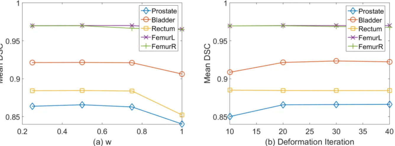
3.10 Sensitivity analysis of task weight w and deformation iteration . . . 64
3.11 Comparison with regression forest in deformation field estimation . . . 66
3.12 Comparison with classification forest in deformation field estimation . . . 68
3.13 Comparison with classification forest on deformation field smoothness . . . . 69
3.14 Bounding-box-based initializations of pelvic organs . . . 72
4.1 Seven prostate anatomical landmarks . . . 80
4.2 The flowchart of treatment-CT segmentation . . . 81
4.4 Inter- and intra-patient shape and appearance variations . . . 85
4.5 Incrementally learned anatomy detector. . . 87
4.6 A schematic illustration of differences among PPAT, IL and ILSM. . . 88
4.7 Multi-atlas RANSAC for robust prostate localization . . . 92
4.8 14 Haar templates used in anatomy detection . . . 97
4.9 DSC differences between ILSM and PPAT for convergence analysis . . . 102
4.10 Comparison between single-atlas and multi-atlas RANSAC . . . 103
4.11 Overlapped prostate contours after bone alignment . . . 105
LIST OF ALGORITHMS
3.1 Regression-based Hierarchical Deformation . . . 56
4.1 Backward pruning algorithm. . . 86
4.2 Forward learning algorithm. . . 87
LIST OF ABBREVIATIONS
2D Two Dimensional
3D Three Dimensional
AP Apex Center
AT Anterior Point
ASD Average Surface Distance ASM Active Shape Model
BS Base Center
CDM Classification based Deformable Model
CT Computed Tomography
DSC Dice Similarity Coefficient
FOV Field of View
IGRT Image-guided Radiotherapy IL Incremental Learning
ILSM Incremental Learning with Selective Memory LF Left Lateral Point
MIX Mixture Learning with Patient-specific and Population Data
MR Magnetic Resonance
PC Prostate Center
PCA Principal Component Analysis POP Population Learning
PT Posterior Point
SEN Sensitivity
SBRT Stereotactic Body Radiation Therapy RANSAC Random Sample Consensus
RDM Regression-based Deformable Model RT Right Lateral Point
CHAPTER 1 : INTRODUCTION
1.1 Image Guided Radiotherapy
Figure 1.1: Illustration of image guided radiotherapy
IGRT increases the probability of tumor control and reduces the possibility of side effects. [Xing et al., 2006, Dawson and Jaffray, 2007].
There are two segmentation problems in the IGRT, planning-CT segmentation and treatment-CT segmentation. The efficacy of IGRT depends on the accuracy of both seg-mentations.
• Treatment-CT segmentation aims to accurately and quickly localize the prostate in daily treatment CT images. The segmentation can be used for three purposes. 1) The segmentation can be used to guide radiation treatment. Based on the prostate segmen-tation, the treatment plan can be aligned from the planning image space to the current treatment image space for precisely targeting the current anatomy of the prostate. 2) The segmentation can be used to calculate the dose accumulation. By deformably reg-istering daily treatment images to the planning image space based on the segmented structures, the accumulation of radiation dose over the past treatment period can be calculated in the pelvic region. This dose accumulation provides feedbacks in the adaptive radiotherapy that can be used to modify the treatment plan for improving radiation treatment at follow-up fractions. 3) The segmentation can be used to tell whether a significant change of anatomy happens and whether a re-optimization of treatment plan is necessary. In this dissertation, the first purpose is the main focus of treatment-CT segmentation. As the segmentation is used to guide the daily treat-ment, besides accuracy, efficiency is also important for treatment-CT segmentation. If an algorithm is computationally expensive, the anatomical structures in the area of interest may have changed during the computation, which could invalidate the purpose of segmentation.
is clinically desirable to develop a robust, accurate and automatic algorithm for planning-CT and treatment-CT segmentation.
The following sections are organized as follows. Section 1.2 presents the challenges in de-veloping automatic methods for segmenting male pelvic organs in CT images. Section 1.3 and section 1.4 summarize the existing methods for planning-CT segmentation and treatment-CT segmentation, respectively. Their limitations are also discussed. Section 1.5 presents the contributions of this dissertation in both planning and treatment-CT segmentation. Section 1.6 gives a brief overview of the remaining chapters. The summary of this chapter is given in section 1.7.
1.2 Challenges of Automatic Segmentation
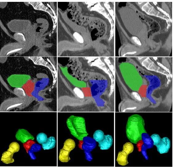
It is generally difficult to automatically segment male pelvic organs from CT images due to three challenges as illustrated in fig. 1.2. 1) Certain parts of pelvic organ boundaries exhibit low contrast in CT images, such as the prostate boundaries, the rectum boundaries and the touching boundaries between the bladder and the prostate. 2) The shapes of the bladder and rectum are highly variable. They can change significantly across patients and between CTs of one patient himself due to different amounts of urine in the bladder and bowel gas in the rectum. 3) Not only is the shape of the rectum variable due to the bowel gas, but also is the appearance of the rectum.
Figure 1.2: Typical CT scan slices and their pelvic organ segmentations. The three columns indicate images from three patients. The first, second, and third rows show, respectively, a sagittal CT slice, the same slice overlaid with segmentations, and a 3D view of segmentations of each patient. Red: Prostate; Green: Bladder; Blue: Rectum; Yellow: Left femoral head; Cyan: Right femoral head.
the textures of major pelvic organs. The diversity of pelvic CT images, in addition to the anatomical variations, further complicates the segmentation of male pelvic organs from CT images.
1.3 Planning-CT Segmentation
segmentation. Few methods were based on deformable image registration. The reasons are attributed to the diversity of pelvic CT images and large anatomical variation. As shown in fig. 1.2, large anatomical variations cause significant differences in shapes and appearances of pelvic organs across subjects. These make registration between CT images of different subjects very difficult. In addition, CT images of different subjects may be acquired with different fields of view, with/without contrast agent, and with/without metal implants. These differences make the correspondence detection challenging even in image registration. In contrast, deformable models suffer less from these problems, once they are well initialized. They can potentially overcome problems caused by image noise and artifacts by imposing the global shape constraint during segmentation. Besides, deformable models are usually more efficient than deformable image registration, since most of them only operate on the organ boundary instead of the entire image domain. These reasons make deformable models popular in planning-CT segmentation.
1.3.1 Previous Work
spatial relationship between nearby organs, many methods imposed additional constraints in the shape matching term to improve the robustness of segmentation. For example, [Rous-son et al., 2005] proposed a Bayesian formulation that considers the non-overlapping con-straint to segment the prostate and rectum. [Pizer et al., 2005] proposed a medial shape model named M-reps for joint segmentation of the prostate, bladder and rectum. [Costa et al., 2007] proposed coupled 3D deformable models to segment the prostate and bladder by considering an asymmetric non-overlapping constraint. [Chen et al., 2011] incorporated anatomical constraints from pelvic bones into a Bayesian framework for jointly segmenting the prostate and rectum. Instead of using intensity/gradient to define the image matching term, recently machine learning techniques have been proposed to characterize the matching of organ boundary. For example, [Lu et al., 2012] detected the boundaries of pelvic organs by using probabilistic boosting trees together with a Jensen-Shannon divergence-based mea-surement. To improve the robustness of deformable model initialization, [Lay et al., 2013] proposed to learn global image context for fast localization of pelvic organs. The initial-ized shape model is then refined iteratively by a discriminantive learned boundary detector, similar to the way done in [Lu et al., 2012].
planning system calledPinnacle [Koninklijke Philips N.V., 2016] that provides a module for automatic segmentation of pelvic organs in CT images. The method implemented in the module is based on deformable models that use image gradients to drive shape models onto organ boundaries. If interested, readers may refer to [Chaney and Pizer, 2016] for detailed descriptions of the use of deformable models in commercial products.
1.3.2 Limitations of Previous Work
In deformable models, the image matching term is often defined using intensity profile, gradient profile, regional histogram of intensity and regional histogram of gradient. Besides, the quantitle function was also used in the literature [Broadhurst et al., 2006]. Compared to the regional histogram, the quantitle function shows better properties for statistical analysis, such as for principal component analysis. All these definitions of the image matching term work well for segmenting organs with distinctive intensity patterns and clear boundaries. However, their performance is limited in the segmentation of CT pelvic organs, because 1) the intensity distributions of different pelvic organs can be similar, and 2) the boundaries of pelvic organs are unclear. While these limitations can be overcome by using a classifier to learn discriminative boundary patterns of pelvic organs [Lu et al., 2012, Lay et al., 2013], the existing deformable models still suffer several intrinsic problems, which make them ineffective in the planning-CT segmentation.
However, in the case of pelvic organ segmentation, where inter-subject anatomical variations are large, it is often difficult to obtain a good initialization. Therefore, the performance of existing deformable models is limited.
• Tubular Organs. Deformable models have difficulty in segmenting tubular organs, such as the rectum. The contributing reasons are 1) initialization and 2) local search range. First, it is hard to initialize a shape model for tubular organs due to their large shape variation. Second, it is tricky to find an appropriate value for local search range during shape deformation. A small local search range prevents sufficient deformations for an initialized shape model to attach the organ boundary, while a large local search range can easily cause mesh folding or shrinkage because the left boundary of shape model may find high boundary responses on the right tube wall.
To overcome the aforementioned limitations, it is necessary to propose a new deformation mechanism for deformable models that is robust to arbitrary initialization and flexible to segment tubular organs.
1.4 Treatment-CT Segmentation
can exploit these additional data to learn patient-specific characteristics and improve the segmentation accuracy.
It is noteworthy that instead of acquiring a treatment CT image the prostate location at each treatment day can also be accurately approximated using implanted markers. Such marker tracking techniques, using either radiofrequency or 2D planar images, can reduce the radiation dose to the patient from CT imaging. However, the lack of volumetric image data prevents calculation of delivered dose on structures as desired in adaptive radiotherapy. To overcome this problem, [Lee et al., 2010] proposed to estimate the treatment image by mapping planning image data to the treatment space via the deformation field estimated using the implanted markers. They showed that the calculated dose histograms using the estimated images are close to those using real treatment images. However, this technique is still under research and has not been widely adopted in the clinic. Besides, markers need to be implanted inside the prostate, which may cause complications such as urinary tract infection [Shinohara and Roach, 2007]. Therefore, this dissertation still considers the conventional scenario where a treatment image is acquired for localizing the prostate at each treatment day.
1.4.1 Previous Work
prostate localization. Besides, the registration also benefits voxel-wise labeling, which can be performed only in a small region around the roughly localized prostate. It not only increases computational efficiency but also allows classifiers to be specifically trained for labeling voxels near the prostate, thus improving labeling accuracy. In the following paragraphs, existing methods based on deformable registration and voxel-wise labeling are respectively discussed.
the bowel gas, are automatically filtered out, which makes registration more robust. To account for registration errors, [Liao et al., 2013] further proposed a patch-based label fusion framework, which uses sparse representation to identify similar voxels from warped CT images of the same patient and propagates only their labels for prostate localization.
• Voxel-wise labeling labels each voxel in the image based on local image appearance. It learns a strong classifier to distinguish voxels inside the target organ (positives) from those outside (negatives), according to the segmented training images. Once learned, the classifier is applied voxel-wisely to produce an organ likelihood map for a testing image, where the target organ is enhanced and can be easily segmented by either thresholding or simple segmentation methods. For example, [Li et al., 2012] proposed to utilize context information to iteratively refine the voxel-wise labeling result. Then, a level set was used to segment the prostate from the labeling map. [Gao et al., 2012a] proposed a sparse representation based classifier and employed multi-atlas labeling for prostate segmentation. To utilize valuable information from manual interactions, [Shi et al., 2013] proposed a semi-supervised learning framework that learns a classifier by integrating information from both manual interactions and previous segmented image data.
1.4.2 Limitations of Previous Work
treat-ment. Therefore, treatment-CT segmentation demands higher segmentation efficiency than planning-CT segmentation. However, the existing methods are too slow to meet this need. For example, in deformable registration based methods it typically takes minutes or even longer to register an atlas to a treatment CT image. In the case when multiple atlases are used, the time for registration would be even longer. In voxel-wise labeling, efficiency is often limited by using a complex classifier [Gao et al., 2012a] or performing iterative classification refinement [Li et al., 2012]. The long localization procedure makes the existing methods inapplicable to image guided radiotherapy, although they are still useful in the adaptive radiotherapy where the segmentation can be conducted offline.
Besides expensive computations, voxel-wise labeling methods [Li et al., 2012, Gao et al., 2012a, Shi et al., 2013] suffer another limitation. They require at least three patient-specific images manually segmented for learning a classifier. This requirement imposes additional burdens on radiation oncologists, as manual segmentation is time consuming (10 minutes for the prostate). Moreover, there may be no sufficient patient-specific data available, especially in the beginning treatment day when only one planning image is available.
To overcome the above limitations, it is necessary to develop a fast segmentation method that meets the following requirements. The method should rely on little manual delineation and be robust when the amount of patient-specific data is limited, such as in the beginning of treatment days.
1.5 Thesis
Thesis: Deformable models benefit in accuracy from explicitly learning deformations from
image appearance. Landmarks can be utilized for fast and accurate segmentation of treatment
cascade learning framework.
This dissertation investigates solutions to address the limitations of existing methods in planning-CT and treatment-CT segmentations, and it proposes new algorithms for accurate and efficient segmentation of male pelvic organs from CT images. The dissertation focuses on improving not only the accuracy of segmentation algorithms but also the processing efficiency. In particular, two specific aims are proposed.
• Specific Aim 1 (Planning-CT segmentation). The accuracy of deformable mod-els can be improved by explicitly learning deformations from image appearance. Many conventional deformable models rely on local search to drive shape models onto organ boundaries. This deformation mechanism makes them sensitive to initialization and also limits their flexibility to segment tubular organs, such as the rectum. Since image appearance is informative to the anatomical location in the image, the direction and distance from any voxel to the boundary of target organ can be potentially predicted based on the appearance of local image patch. This information can be used as de-formation to guide the move of shape model toward the organ boundary, which could effectively address the limitations of conventional deformable models.
• Specific Aim 2 (Treatment-CT segmentation). Landmarks can be utilized for fast and accurate segmentation of treatment CTs by effectively combining limited
effi-ciency and reduce effort of manual annotation, anatomical landmarks can be used for segmentation, since they are efficient to detect and easy to annotate. In landmark-based segmentation, anatomical landmarks are first detected on a new image and then used to guide the registration between existing segmented images and the new image. After registration, the existing segmentations are aligned onto the new image space, where the final segmentation is obtained by a label fusion method, such as the majority voting. The efficiency and accuracy of landmark-based segmentation depend on the landmark detection. While it is efficient to detect landmarks using the cascade learning framework, the accuracy could be limited if the landmark detectors are learned from massive population data because of large inter-patient anatomical variation. On the other hand, it is also infeasible to learn from limited patient-specific data; doing so tends to suffer from the overfitting problem. To this end, an effective strategy should be explored to combine limited patient-specific data with massive population data in the cascade learning framework.
In order to support the thesis and the above two specific aims, the detailed contributions of this dissertation include
• A novel deformable model, namely a regression-based deformable model, is proposed
to hierarchically deform a shape model onto the target organ boundary based on an explicitly learned deformation field;(Aim 1)
• An auto-context model is adopted to iteratively refine the predicted deformation field
by gradually incorporating the neighborhood prediction information; (Aim 1)
ap-pearance by coupling deformation regression and organ classification in a common random forest; (Aim 1)
• A multi-resolution strategy is adopted to segment multiple pelvic organs from CT images, where the coarse-level deformation fields are jointly estimated for all organs to consider their spatial relationship and where the fine-level deformation fields are separately estimated for each organ to make the respective prediction models specific; (Aim 1)
• Extensive experiments on a large prostate CT dataset (>300 patients) show that the proposed method can accurately segment the prostate, bladder, rectum and two femoral heads from planning CT images and that it outperforms many existing methods in this task;(Aim 1)
• Thecascade learning framework is adapted to address the problem of unbalanced
train-ing samples in the classification-based landmark detection. It can efficiently localize a landmark in a 3D medical image volume within one second using a multi-resolution implementation; (Aim 2)
• An incremental learning scheme, namely incremental learning with selective memory,
is proposed to update the existing landmark detector learned from massive population data with limited patient-specific data. It can be used to personalize the population-based landmark detectors to a specific patient; (Aim 2)
• Random sample consensus (RANSAC) is used to align the previous segmentations of the same patient onto the target treatment image by considering the possibility of mis-detected landmarks; (Aim 2)
• Extensive experiments on a large prostate CT dataset (> 400 treatment CT images)
show that the proposed method is able to accurately localize the prostate in treatment CTs within 4 seconds; the method satisfies the accuracy and efficiency requirement of IGRT. (Aim 2)
1.6 Overview of Chapters
The remaining chapters of this dissertation are organized as follows.
• Chapter 2 presents the background of related techniques and evaluation metrics used in the dissertation. The techniques include random forests and deformable models. Under random forests, the basics and mathematical notations are presented, followed by the application of random forests to multi-class classification and multi-variate regression problems. Under deformable models, the active shape model is elaborated, as it is closely related to the proposed regression-based deformable model. Finally, several evaluation metrics are given. They are used to evaluate the proposed segmentation methods and compare them with other existing methods.
• Chapter 3 presents regression-based deformable models (RDM) for planning-CT
field, two techniques are presented. First, an auto-context model is proposed to itera-tively refine the estimated deformation field by exploiting local structured information. Second, a multitask random forest is proposed to couple deformation regression with organ classification. Compared to a random forest trained only for deformation regres-sion, the multitask random forest is able to improve the robustness of deformation field estimation by exploiting information from organ classification. Extensive experimental results are given to evaluate each design of the segmentation method and to show the superior performance of the proposed method over several existing methods.
• Chapter 4 presents a fast landmark-based approach for treatment-CT segmentation.
To efficiently detect a landmark, the detection problem is formulated as a binary clas-sification problem, where positives and negatives are voxels near and far away from the annotated landmark, respectively. To handle the highly imbalanced training sam-ples (i.e., limited positives and unlimited negatives), a cascade learning framework is presented to gradually separate negatives from positives. Due to large inter-patient anatomical variations, the classic population-based cascade learning doesn’t perform well. To improve its performance, a novel learning scheme, namely incremental learn-ing with selective memory (ILSM), is proposed to update cascade classifiers learned from a population with limited patient-specific data. Extensive experiments show the effectiveness of ILSM over other learning schemes. Comparing with existing meth-ods, ILSM reduces runtime to seconds while maintaining competitive segmentation accuracy.
• Chapter 5 concludes the dissertation and discusses the limitations of the proposed
dissertation for planning-CT and treatment-CT segmentation are briefly summarized. Their limitations are also discussed. In the future work, interesting future directions are discussed, which include several potential strategies to improve the proposed methods.
1.7 Summary
CHAPTER 2 : BACKGROUND
2.1 Random Forests
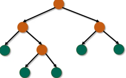
Random forests are general machine learning methods for supervised learning, e.g., clas-sification and regression. Random forests are popular in computer vision and medical image analysis [Criminisi and Shotton, 2013] due to their high efficiency and good scalability. A random forest consists of multiple binary decision trees. Each decision tree consists of two types of nodes: split node and leaf node. Fig. 2.1 gives the visualization of the two types of nodes in a binary decision tree. The split nodes are interior nodes in a decision tree. Each of them is associated with a binary split function, which routes a given sample either to its left or right child node based on a tuple of descriptors. These descriptors are called features in the machine learning field. The leaf nodes are terminal nodes in a decision tree. Each of them stores the information of training samples routed to it. This information is used for prediction of a new testing sample.
Figure 2.1: A decision tree in a random forest.
2.1.1 Training of Random Forests
As an ensemble model, each decision tree in a random forest is trained independently. To increase the diversity of decision trees, a different training subset is randomly sampled with replacement from the entire training set to train each tree. Studies [Breiman, 2001, Liu et al., 2005] show that high diversity prevents overfitting and usually leads to lower generalization error.
Decision Tree Prediction. Given a sampled training set, a decision tree is trained re-cursively starting with the root node. Each node learns the optimal split function that separates the arrival training set into two subsets by maximizing the purity of each split subset. Mathematically, the optimal split function is found by maximizing the following objective function:
arg max
φ∈Φ
1 |SL|
P(SL) +
1 |SR|
P(SR), (2.1)
where S is the training set arriving at this node, SL and SR are the subsets split to the
left and right child nodes, respectively, P(.) calculates the purity of a training set, f(s|φ) is a binary split function with parameters φ, and Φ is a candidate parameter set. In the classic random forests, a decision stump is used as the split function due to its efficiency. Mathematically, a decision stump is formulated as f(s|φ) = s(i) > t, where i is a feature index, t is a threshold, and s(i) extracts the i-th feature of sample s.
To solve eq. 2.1, a random set of split functions is first generated, e.g., by randomizing feature index i and threshold t, and then exhaustive search is used to find the optimal split function in the random set that maximizes eq. 2.1. Afterwards, the training set S is divided into two subsets SL and SR according to the learned split function, and then the
same procedure is performed to further split each subset into smaller ones with more purity. This recursive process stops when 1) the decision tree reaches a predefined maximum tree depth, or 2) the training set S is too small to be split, or 3) the purity within a node is above a threshold. When a split stops, the corresponding node is made as a leaf node, and the training set that arrives the node is stored there. Practically, it is memory inefficient to store training samples in the leaf nodes. Therefore, only the task-specific statistics of a training set are stored.
2.1.2 Application of Random Forests
Given a target sample, the prediction of each decision tree in a random forest is inde-pendent. The final prediction of a random forest is the average prediction over all decision trees.
Specifically, the testing sample is routed to the left child node if f(s|φ) = 0 and to the right child node if f(s|φ) = 1. When a leaf node is reached, the task-specific statistics stored in it are retrieved for prediction.
2.1.3 Random Forest Classification and Regression
Random forests are general to many supervised learning tasks [Criminisi et al., 2011]. To adapt a random forest to a specific task, the purity function P(.) and the task-specific statistics need to be defined. In this subsection, multiclass classification and multivariate regression are taken as two examples to show how random forests can be used to solve general supervised learning problems.
Multiclass Classification. Classification is the prediction of a discrete variable, called the label, from a tuple of features. In classification the purity function P(.) is defined based on the labels of training samples. It encourages each decision tree to partition a training set into subsets with the same label. Therefore, the purity function in the classification measures the label consistency of a training set. It can be quantified by the negative entropy E.
E(S) =X
c
pclogpc, (2.3)
wherepcdenotes the percentage of training samples with the labelcin a training setS. The
larger E(S), the purer the training setS is in terms of the class label.
entry in the label distribution indicates the likelihood of the testing sample belonging to one class. Finally, the label of the testing sample is determined as the class with the maximum likelihood.
Multivariate Regression. Regression is the prediction of a continuous variable, called the regression target, from a tuple of features. The regression target can be a scalar or a vector. In regression the purity function P(.) is defined based on the regression targets of the training samples. It encourages each decision tree to partition a training set into subsets with similar regression targets. Therefore, the purity function in regression measures the consistency of regression targets in a training set. It can be quantified by the summation of negative variances at different dimensions of regression target.
V(S) = −X
k
vk, (2.4)
where vk measures the variance of regression targets at thek-th dimension in a training set
S. The larger V(S) is, the purer the training set S is in terms of the regression targets. In the regression task each leaf node stores the average regression target of training samples that arrive at this node. In the testing stage, when a testing sample arrives at a leaf node of one decision tree, the average regression target is retrieved from the leaf node to serve as the prediction output for the decision tree. Given a group of decision trees in a random forest, the prediction of a forest is the averaged output across all decision trees.
2.1.4 Advantages
Efficiency
Most machine learning models (e.g., the support vector machine) decouples feature ex-traction from model prediction. Regardless of the importance, all features have to be com-puted before the learned model can be applied for prediction. This makes the testing time linear with the feature dimension. As the feature dimension is often large in real applications (e.g., thousands), efficiency becomes a concern for most machine learning methods. In the field of image analysis, this concern is aggravated if the prediction is performed on the voxel level.
Scalability
Scalability is an important factor when choosing a machine learning algorithm for image analysis because each voxel is a training sample and potentially millions of training samples can be collected for training. To fit the massive training samples well, the learned model should have a reasonably large model complexity. However, a large model complexity often means a high computational complexity for most learning models.
Random forests scale well with massive training samples. As each leaf node outputs a unique prediction, the model complexity of a random forest can be approximated by the number of leaves in a decision tree. Since the number of leaves grows exponentially with the tree depth, a random forest with a limited tree depth (e.g., 20-40) is often sufficient to fit millions of training samples with a negligible impact on the runtime efficiency.
Nonlinearity
Prediction with image data often involves learning a highly nonlinear mapping from image features to either a discrete variable in the classification or a continuous variable in the regression. Due to this nature of nonlinearity, linear models often do not work well with image data. While the kernel tricks [Shawe-Taylor and Cristianini, 2004] can often be used to adapt linear models for nonlinear predictions, they don’t scale well when a training dataset is large.
the flexibility of random forests in the training and also increases their performance in the testing.
Convenience
Random forests are convenient to use in practice. Different from many learning algo-rithms, random forests don’t require the input features to be normalized. This property makes it easy for random forests to integrate features from multiple sources. The reason for not requiring feature normalization is because each split node uses only one feature and each feature is used independent from others.
In addition, random forests have a limited number of parameters to tune, and the per-formance is quite robust to the choice of parameters due to the combination of multiple independent models. By averaging the prediction results from independent decision trees, the variance of random forests is reduced and so is the risk of overfitting.
2.2 Deformable Models
slower than parametric ones. Among various deformable models, this chapter focuses on a particular parametric deformable model called the “active shape model” (ASM) [Cootes et al., 1995] as it is closely related to the regression-based deformable model proposed in chapter 3. Discussions of other deformable models are beyond the scope of this dissertation. ASM is popular in the field of medical image segmentation. In ASM a shape is repre-sented by a collection of points. The segmentation is conducted by iteratively deforming a shape toward the boundary of target object. Different from other deformable models [Kass et al., 1988], which impose only a local smoothness constraint on the deformed shape, the deformation of ASM is constrained in a global shape space. The global shape constraint in-creases the robustness of segmentation and makes ASM a useful tool for organ segmentation in noisy and low-contrast medical images.
The ASM algorithm has two stages: a training stage and an application stage. The training stage is detailed in section 2.2.1, where a statistical shape space is learned from segmented training images. The application stage is described in section 2.2.2, which shows how the mean shape is iteratively deformed to fit the boundary of target object under the constraint from the learned shape space. Finally, section 2.2.3 discusses the limitations of ASM.
segmentation.
2.2.1 Training of the Active Shape Model
The training part of the ASM algorithm aims to learn a statistical shape space that captures the mean and variation of the shapes of target object from segmented training images. Two steps are performed to learn a shape space: 1) building shape correspondence across subjects and 2) principal component analysis of correspondent shapes. Both steps are elaborated below.
Shape Correspondence
A shape in the 3D ASM is often represented by a triangle mesh. Two shapes are in correspondence if 1) they have the same number of vertices and 2) vertices with the same index correspond to roughly the same anatomical location. In the 2D ASM the shape correspondence is often built by manually annotating landmarks along the boundary of target object. However, manual annotation is burdensome for building shape correspondence in the 3D ASM, as a triangle mesh often consists of thousands of vertices. To reduce the manual efforts, an automatic procedure is necessary for building the shape correspondence in the 3D space. While there are sophisticated methods out there, e.g., those based on entropy or description length [Davies et al., 2001, Davies et al., 2010, Cates et al., 2007], the following paragraphs describe a simple method for building the shape correspondence.
The method starts with constructing a reference shape and then registers it to individual shapes for building the shape correspondence across subjects.
be done by simply selecting an arbitrary binary segmentation image. However, doing so may introduce biases. To overcome potential biases, the Fr´echet mean image [Joshi et al., 2004, Fletcher et al., 2009] can be computed and used as the template image space; 2) all binary segmentation images are linearly aligned onto the template image space using a similarity transform; 3) all aligned binary segmentation images are voxel-wisely averaged to form a mean segmentation image. To construct the reference shape, the marching cubes algorithm [Lorensen and Cline, 1987] is first adopted to extract a dense mesh from the mean segmentation image. Afterwards, mesh decimation and remeshing are alternately performed to reduce the number of vertices to a manageable size (e.g., 1000-2000) while keeping all vertices evenly distributed on the surface. The final triangle mesh after mesh decimation is used as the reference shape.
• Surface Registration. To build the shape correspondence across subjects, the dense triangle mesh of each subject is first extracted from its segmentation image using the marching cubes algorithm. Then, the reference shape is non-rigidly registered to each dense mesh by a robust surface registration algorithm [Myronenko and Song, 2010]. Since all registered reference shapes come from a single source and fit individual shapes well, these shapes are in correspondence and can be used for learning a statistical shape space.
Principal Component Analysis
principal component analysis (PCA) is adopted to compute the variation modes by an eigen-decomposition of the covariance matrix.
C= 1 N −1
N
X
i=1
(ui−u)(u¯ i −u)¯ T, (2.5)
{ck,ek}= eign(C), (2.6)
where N is the number of shapes, ui is the i-th aligned shape, ¯u is the sample mean shape,
C is the covariance matrix, and ck and ek are the k-th eigen-value and eigen-vector of
the covariance matrix C. The output of principal component analysis gives a statistical shape space described by a multivariate Gaussian distribution with the mean ¯u and the variation modes {ck,ek}. In practice, only the K eigen-modes with the largest eigen-values
are preserved to make the shape space compact. Although eigen-values can be affected by noise, a common practice to select K is still based on the eigen-values. Specifically, K is often selected as the minimum number of eigen-modes that account for the majority of shape variations, i.e., minK, s.t. (PK
k=1ck/
P
kck)> , where is often chosen as a value close to
100%, such as 90%.
2.2.2 Application of the Active Shape Model
Each iteration involves two steps: 1) vertex-wise local deformation and 2) global refinement by the statistical shape space.
Vertex-wise Local Deformation
As shown in fig. 2.2, each vertex of the shape locally searches along its normal direction and finds a position most likely to be the object boundary. Then, the vertex is deformed to the boundary position.
There are many ways to characterize the object boundary. A simple way is to use the image gradient magnitude based on the assumption that voxels with large gradient magnitudes are more likely to be on the object boundary than those with small gradient magnitudes. While this strategy works well for objects with clear boundaries, it fails notably if the object boundary is indistinct, such as the boundaries of pelvic organs in CT images. Recently there is a trend that detects the object boundary by learning a classifier based on local image features. Since the patterns of object boundary are learned from multiple local image features, it is often more effective than using simple gradient magnitudes.
Global Refinement by the Shape Space
Figure 2.2: Illustration of vertex deformation in the active shape model. The purple area is the target object; the yellow dashed line indicates the current location of shape model; the red points are the boundary points (vertices) on the shape model; the blue line shows the normal direction of one vertex; the orange point shows the position along the normal direction with the maximal boundary response.
shape space, and the final segmentation is plausible and looks like those observed in the training set. The following mathematical equations explain how to find the closest shape ˆut
in the shape space for a given shape ut.
αk = (ut−u)¯ Tek, γ = max(1,
1 T
X
k
α2 k
ck
), (2.7)
ˆ
ut= ¯u+
1 γ
X
k
αkek, (2.8)
whereαkis thek-th coefficient of shapeutmapped into the shape space, ¯uis the mean shape,
ck and ek are the k-th eigen-value and eigen-vector of the shape space, T is a predefined
2.2.3 Limitations
With a shape space the deformed shape is always constrained in a plausible shape set learned from training data. This advantage makes ASM well suited for medical image seg-mentation, where image appearance may be unreliable due to noise and artifacts. However, ASM has several limitations that should be addressed before it can be a powerful tool for CT pelvic organ segmentation.
Sensitivity to initialization
Because each vertex is deformed locally, the performance of ASM relies on a good initial-ization. If the shape model is not initialized close to the object boundary, local search won’t be able to find the boundary. However, it can be tricky to automatically and robustly ini-tialize the shape model. In the CT pelvic organ segmentation, the difficulties come from two aspects: 1) it is challenging to accurately detect the position, orientation and size of pelvic organs in CT images due to low contrast and large inter-subject anatomical variation; 2) the mean shape can be dramatically different from individual shapes to segment. This difference renders the mean shape initialization ineffective for organs with large shape variations, such as the rectum.
Inflexibility to Segment Tubular Organs
There are two issues when ASM is applied to segment tubular organs, such as the rectum.
thin organs, such as the rectum. A small local search range is insufficient to find the boundary while a large local search range can cause mesh folding or shrinkage as the vertices on the left tube wall may find the boundary location on the right tube wall. Ideally the local search range should be spatially adaptive. If a vertex is close to the object boundary, its search range should be small. If a vertex is far away from the object boundary, its search range should be large.
• Shape Space. There are three challenges when using a shape space for tubular organ segmentation: 1) the variation of tubular shapes are mostly nonlinear, e.g., twisting and bending, while the PCA shape space captures only linear variations [Cootes et al., 1995]; 2) due to large variations of tubular organs, the number of training data is often limited to sufficiently describe these variations; 3) the shape distribution of tubular organs doesn’t necessarily follow the Gaussian assumption of the PCA shape space.
To overcome these limitations, it is necessary to 1) change the deformation mechanism from local to non-local, thus making deformable models insensitive to initialization; 2) adapt the deformation of each vertex based on its distance to the object boundary, thus addressing the issue of search range; 3) increase the robustness of shape deformation and reduce its dependency on the shape space, as the PCA shape space may not be suitable to describe the shape statistics of tubular organs.
2.3 Segmentation Evaluation
existing methods.
• Dice Similarity Coefficient (DSC). DSC measures the overlap ratio between an automatic segmentation and a manual segmentation. It ranges from 0% to 100%. 0% indicates the worst segmentation and 100% indicates the best segmentation. Mathe-matically DSC is defined as the equation below.
DSC = kVolgt∩Volautok (kVolgtk+kVolautok)/2
, (2.9)
where Volgt and Volauto are the voxel sets of manually labeled and automatically
seg-mented objects, respectively. The values of DSC vary strongly with both object size and shape. It is more difficult for automatic segmentation methods to achieve high values of DSC on objects with small sizes and elongated shapes than those with large sizes and sphere-like shapes.
• Average Surface Distance (ASD). ASD measures the average distance between the
surfaces of an automatic segmentation and a manual segmentation. Mathematically it is defined as the equation below.
ASD = 1 2 mean a∈Volgt min b∈Volauto
d(a, b) + mean
a∈Volauto min b∈Volgt d(a, b) , (2.10)
Among various surface distance metrics, ASD is only one of them. Besides ASD, an-other commonly used surface distance metric is Hausdorff distance. Hausdorff distance has a similar definition with ASD except that Hausdorff distance computes the 90 per-centile of surface distances instead of taking the mean as done in eq. 2.10. Therefore, Hausdorff distance is more sensitive to local variations than ASD. However, as ASD is more frequently used in the literature of CT pelvic organ segmentation than Hausdorff distance, this dissertation reports only the values of ASD for the purpose of comparison.
• Sensitivity (SEN) and Positive Predictive Value (PPV).SEN measures the percentage of a manual segmentation that overlaps with an automatic segmentation, and PPV measures the percentage of an automatic segmentation that overlaps with a manual segmentation. These two metrics are informative to over-segmentation and under-segmentation. In the case of over-segmentation, SEN is high and PPV is low. In the case of under-segmentation, SEN is low and PPV is high. Mathematically they are defined as the equations below.
SEN = kVolgt∩Volautok kVolgtk
, (2.11)
PPV = kVolgt∩Volautok kVolautok
. (2.12)
2.4 Summary
CHAPTER 3 : LEARNING DEFORMATIONS FOR PLANNING-CT SEGMENTATION
As mentioned in section 1.3.2, conventional deformable models are sensitive to initializa-tion and ineffective for segmenting tubular organs. These limitainitializa-tions make them not well suited for CT pelvic organ segmentation, where robust initialization of deformable models is difficult and organs may have tubular shapes, e.g., the rectum. To overcome these limita-tions, this chapter investigates a novel deformable model named“regression-based deformable model” (RDM) 1 to segment male pelvic organs from CT images; these organs include the
prostate, bladder, rectum and two femoral heads. In RDM, a deformation field toward an organ boundary is predicted from an intensity image by a regression model. It is used to explicitly guide a deformable model for segmentation. Compared to conventional deformable models, the estimated deformation field in RDM provides non-local deformations. Guided by these deformations, RDMs are insensitive to initialization. Moreover, as deformations become spatially adaptive, RDMs are more flexible than conventional deformable models to segment tubular organs. These properties render RDMs appealing for CT pelvic organ segmentation.
To accurately and robustly estimate the deformation field for a RDM, this chapter in-vestigates two novel machine learning techniques as briefly summarized below and detailed in sections 3.1 and 3.2, respectively.
• Auto-context Model. In conventional voxel-wise prediction, the deformation at one voxel is independently predicted without considering those of its neighborhood. As deformations in the spatial neighborhood are highly correlated, the independent estimation often results in a noisy and spatially inconsistent deformation field. To improve the prediction accuracy,an auto-context model is adopted to iteratively refine the deformation field by considering not only local image appearance but also predicted deformations at neighboring voxels. A synthetic experiment shows that the auto-context model captures the structured information in the spatial neighborhood. This information is useful to suppress prediction noise and improve the spatial consistency of deformation field.
multitask random forest improves the robustness of deformation field estimation.
With the above techniques, a deformation field can be predicted for a target image and used to guide deformable segmentation. However, it is risky to deform the shape model directly using the estimated deformation field because of potential mis-predictions. To fur-ther improve the robustness of deformation, two strategies are proposed in sections 3.3 and 3.4, respectively. Section 3.3 proposes a hierarchical deformation strategy where the shape deformation is highly constrained in the beginning and gradually relaxed as the shape model approaches the object boundary. Section 3.4 investigates a multi-resolution segmentation framework where multiple organs are jointly segmented in the coarse resolutions, and their segmentations are separately refined in the fine resolutions.
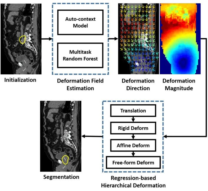
Fig. 3.1 shows the flowchart of the proposed method for planning-CT segmentation, which consists of three major components: for deformation field estimation, 1) the auto-context model; 2) the multitask random forest; and 3) for organ segmentation, regression-based hierarchical deformation. Each step will be detailed in the following sections.
3.1 Deformation Regression and Auto-context
3.1.1 Deformation and Deformation Regression
In RDM, as illustrated in fig. 3.2, the deformation at one voxel is defined as the 3D displacement vector from this voxel to the nearest voxel on the organ boundary. Given a testing image with an unknown organ boundary, the deformation at any image location needs to be predicted based on local image appearance. Deformation regression aims to learn a mapping from local appearance features to the deformation based on a set of training images, where manual contours of the target organ are available. At runtime, the learned mapping is applied to predicting the deformations in the testing image, where no manual contour is available.
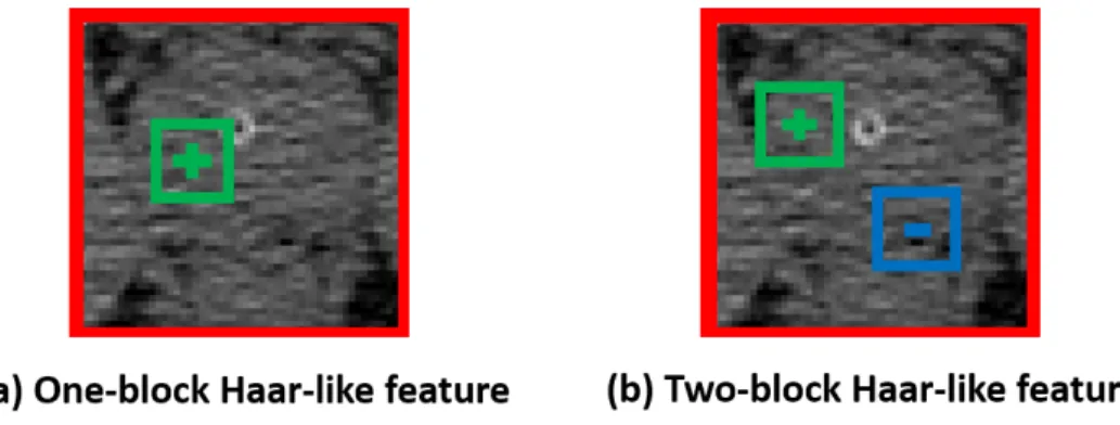
Figure 3.2: Illustration of deformations at several voxel positions. The blue arrows denote the deformations at several voxel positions (yellow crosses) toward the organ boundary (red). The green dashed boxes indicate the local image patches centered at these voxels, where appearance features are extracted.
appearance features (i.e., Haar-like features) and associated with the ground truth defor-mation calculated from the manual contour. These voxels serve as training samples to a random forest, and the random forest is able to learn a regression model that predicts the deformation at any voxel based on local appearance features. The learned random forest is named as “regression forest”, since it is specifically trained for deformation regression.
Given a learned regression forest, the deformation field of a testing image can be esti-mated by independently predicting the deformation at each voxel location. However, such an approach ignores the fact that deformations at neighboring voxels are highly correlated. As a result, the estimated deformation field is often noisy and spatially inconsistent, as shown in the first row of fig. 3.3.
3.1.2 Auto-context Model
To overcome this drawback, deformations predicted at neighboring voxels need to be considered during the voxel-wise estimation of a deformation field. In this work, the auto-context model [Tu and Bai, 2010] is used for this purpose.
The auto-context model was originally proposed in [Tu and Bai, 2010] as an iterative approach for refining the likelihood map from voxel-wise classification. The idea is to consider not only local image appearance but also neighboring classification results during voxel-wise classification. By combining these two pieces of information, the auto-context model is shown to be effective in improving classification results. It is not difficult to see that the same idea can also be borrowed to refine the deformation field from voxel-wise regression. To be specific, the following paragraphs describe the training and testing of the auto-context model when it is applied to refining the deformation field.
• Auto-context Training. The training of the auto-context model typically takes several iterations, e.g., 2-3 iterations. A regressor (e.g., regression forest) is trained at each iteration. In the first iteration, appearance features (i.e., Haar-like features) are extracted from CT image to train the first regressor. Once the first regressor is trained, it is applied back to each training image to generate a tentative deformation field.
Figure 3.4: Schematic diagram of auto-context with n iterations.
estimated deformations at neighboring voxels, it often leads to a better deformation field, as shown in the second row of fig. 3.3.
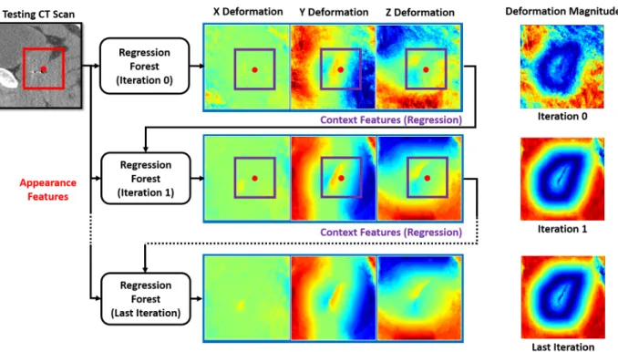
Given a refined deformation field by the second regressor, the context features are updated and can be used together with the appearance features to train the third classifier. The same procedure is repeated until the final iteration is reached. Because each iteration involves voxel-wise classification of all training images, more iterations take longer training time. In practice, 2-3 iterations are often used.
• Auto-context Application. Given a testing CT image, the learned regressors are sequentially applied, as illustrated in fig. 3.3. In the first iteration, the first learned regressor is applied voxel-wise on the testing image to generate a deformation field by using only appearance features. In the second iteration, the second learned regressor is used to predict a new deformation field by combining appearance features from the CT image with context features from the deformation field estimated in the previous iteration. This procedure is repeated until all learned regressors have been applied. The deformation field output by the last regressor is the output of the auto-context model. Fig. 3.4 provides the schematic diagram.
defor-mation field compared to conventional methods that consider only local image appearance (comparing the first and third rows of fig. 3.3).
3.1.3 Understanding the Auto-context Model
The auto-context model differs from conventional voxel-wise prediction methods only in the existence of context features. In this section, it is shown that context features capture neighborhood structured information from training images. This structured information can be enforced by the auto-context model in the prediction map of a testing image.
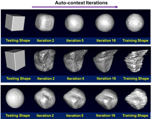
To justify this statement, a synthetic experiment was designed under voxel-wise classifi-cation. In this experiment, given a binary training image that represents a shape, a sequence of random forest classifiers was trained in the same manner as the auto-context model. Then, the learned classifiers were sequentially applied to a testing image with a different shape. The hypothesis is that if the classifiers learn the neighborhood structured information of the training shape the testing shape would generally evolve to be the training shape under the iterative classification. Fig. 3.5 gives the results for three cases, where the training shapes are the sphere, prostate and bladder, respectively. It can be seen that the testing shapes refined by the auto-context model eventually become almost identical to the respective train-ing shapes. This observation indicates that the structured information learned from traintrain-ing images can be enforced in the testing image by the auto-context model. A large number of iterations was used in this experiment to facilitate large shape refinements for the purpose of demonstration. In practice, the refinement won’t be this great since only 2-3 iterations are often used.
Sim-Figure 3.5: Shape refinements by the auto-context model (AC). Upper: sphere. Middle: prostate. Lower: bladder.
ilarly, if the context features were extracted from estimated deformation fields, the auto-context model would learn structured deformation information. The learned structured in-formation is the key ingredient that makes the auto-context model outperform conventional voxel-wise prediction models.
3.2 Multitask Random Forest
are mis-predicted in the spatial neighborhood, the auto-context model would lead to wrong refinements. To relieve this problem, a multitask random forest2 is proposed to replace the
standard regression forest used in the auto-context model. In the multitask random forest, deformation regression is jointly learned with another task, i.e., organ classification, in a single random forest. Organ classification refers to the classification task that uses local appearance features to distinguish voxels inside the organ from those outside.
Compared to the standard regression forest, the multitask random forest has two ad-vantages: 1) through joint learning the multitask random forest is forced to exploit the commonality between deformation regression and organ classification. The exploited com-monality is helpful to reduce the risk of overfitting; 2) by integrating the multitask random forest with the auto-context model, organ classification provides additional context features, i.e., estimated class information in the spatial neighborhood. They are useful to improve the estimated deformation field near the organ boundary when deformations are not well predicted from local appearance features.
3.2.1 Mathematical Definition
To adapt a random forest for multitask learning, the purity of a training setS is modified as follows in order to consider multiple tasks in the learning process.
P(S) = X
i
wi
Pi(S)
Zi , (3.1)
where wi is the weight for the i-th task, Pi(S) is the purity definition for the i-th task, and
{Zi} are coefficients that normalize the purity across different tasks. For each task, Zi is
defined as the task-specific purity of the entire training set, i.e., the purity at the root node. In this work since only two tasks, i.e., deformation regression and organ classification, are considered, the purity definition can be further specialized as follows:
P(S) =wV
DR(S)
ZDR + (1−w)
EOC(S)
ZOC , (3.2)
wherew∈[0,1] is the weight coefficient,VDR is the purity definition for deformation
regres-sion that measures the variation of deformations in a training set S, and EDR is the purity
definition for organ classification that measures the consistency of class labels in a training setS. Their mathematical definitions are given below:
VDR(S) = − 1
|S|tr
X
x∈S
(dx−d)(d¯ x−d)¯ T
, (3.3)
EOC(S) =p
+logp++p−logp−, (3.4)
where tr is the trace operator, dx is the deformation at a training voxel x, ¯d is the mean
deformation in the training setS, andp+andp−are the percentages of positive and negative
and organ likelihood map.
3.2.2 A Better Model for Deformation Regression
As deformation regression and organ classification are jointly learned in a single random forest, the multitask random forest is optimized to select common features and thresholds that are informative to both tasks. As pointed in [Caruana, 1997], sharing the same model among related tasks could improve the generalization. Moreover, it is found in my work that joint learning of deformation regression and organ classification clarifies the ambiguity that exists in the training of the regression forest.
Fig. 3.6 illustrates the ambiguity where two voxels (yellow crosses), i.e., one inside and one outside the organ, have the same deformation toward the organ boundary but have different image appearances. In the regression forest, which is trained only for deformation regression, the training of random forest tries to find image features that group these two voxels in the same leaf node, since they have the same deformation. However, due to dramatic appearance difference, generally it is infeasible to find such features. In the end, the random forest may find meaningless features that happen to well fit the training set but cannot generalize well in the testing. Thus, a risk of overfitting is imposed.
Figure 3.6: Ambiguity in the training of random forest when deformation is used as the only supervised guidance for splitting. The green contour indicates the bladder boundary. Yellow crosses indicate two voxels with the same deformation toward the organ boundary but with different image appearances.
3.2.3 Integration with the Auto-context Model
is useful to deformation field refinement, especially when deformations are not well predicted from local appearance features at the first iteration of the auto-context model.
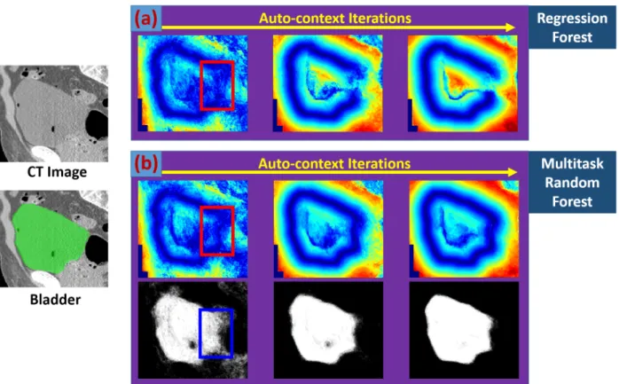
Figure 3.7: Flowchart of the auto-context model with the multitask random forest. The red point indicates a voxel. The red, blue and purple rectangles are the local patches of this voxel on the CT image, estimated organ likelihood maps and deformation fields, respectively.
Fig. 3.8 gives a typical example to illustrate the importance of estimated class information in deformation field refinement. As shown in fig. 3.8(a), if many deformations are mis-predicted in a small region at the first iteration of the auto-context model (red rectangle), the auto-context model is not able to correct them by using context features only from estimated deformation field, since deformations predicted in the neighborhood are also inaccurate. As a result, the deformation field is often generated with missing parts of organ boundaries (fig. 3.8(a)). This problem is called “the missing boundary problem”, which is common if the auto-context model is used with the regression forest.