RECOGNIZING FINE-GRAINED OBJECT INSTANCES FOR ROBOTICS APPLICATIONS
Phil Ammirato
A thesis submitted to the faculty at the University of North Carolina at Chapel Hill in partial fulfillment of the requirements for the degree of Doctor of Philosophy in the Computer Science.
Chapel Hill 2019
ABSTRACT
Phil Ammirato: Recognizing Fine-Grained Object Instances for Robotics Applications (Under the direction of Alexander C. Berg)
State-of-the-art object recognition systems, and computer vision methods in general, are getting better and better at a variety of tasks. Many of these techniques focus on general object categories, like person or bottle, and use many hundreds or thousands of training examples per category. Some domains, such as robotics, require recognition of fine-grained object instances, such as a 16oz. bottle of Coke, and only have access to limited training data.
ACKNOWLEDGEMENTS
I would first like to thank my advisor, Alexander C. Berg, for helping to guide me through my PhD. None of this work would have been possible, especially the data collection, without his encouragement. To Jana Koˇseck´a, thank you for making yourself and your students at George Mason University available for very helpful collaboration. I would also like to thank the other members of my committee, Tamara Berg, Jan-Michael Frahm, and Marc Niethammer, each of which have offered lots of advice and had direct impacts on my research.
My advisors at NVIDIA Research, Jonathan Tremblay, Ming-Yu Liu, and Dieter Fox gave great advice and research ideas throught my time there. My lab mates Adam Aji, Akash Bapat, Marc Eder, Cheng-Yang Fu, Rohit Gupta, Xufeng Han, Dinghuang Ji, Hadi Kiapour, Hyo Jin Kim, John Lim, Wei Liu, Eunbyung Park, Ric Poirson, Johannes Schonberger, Misha Shvets, Sirion Vittayakorn, Thanh Vu, Ke Wang, Zhen Wei, Yi Xu, Licheng Yu, Dongxu Zhao, Enliang Zheng, and Yipin Zhou have all been great to work with, and have made my time at UNC more fun and rewarding. Thank you to all of my other collaborators, including the multiple undergradu-ate groups who built some amazing tools for both my research and their course projects.
I would never have made it through my five plus years here without the amazing staff at UNC, Murray Anderegg, Bil Hays, John Sopko, Missy Wood, Jody Gregoritsch, Denise Kenney, Mike Stone, Mike Carter, Jim Mahaney, and many others.
TABLE OF CONTENTS
LIST OF TABLES . . . ix
LIST OF FIGURES . . . xi
LIST OF ABBREVIATIONS . . . xvii
CHAPTER 1: INTRODUCTION . . . 1
1.1 Thesis Statement . . . 3
1.2 Outline of Contributions . . . 4
CHAPTER 2: TECHNICAL INTRODUCTION . . . 6
2.1 Task Definitions . . . 6
2.2 Neural Networks . . . 8
2.2.1 Basic Overview of a Training Simple Net . . . 9
2.2.2 Convolutional Neural Networks . . . 10
2.3 Object Detection . . . 11
2.4 Generative Adverserial Networks . . . 13
CHAPTER 3: RELATED WORKS . . . 15
3.1 Datasets in Computer Vision . . . 15
3.1.1 Object Pose Datasets . . . 16
3.1.2 Active Focused Datasets . . . 17
3.2 Object Classification. . . 18
3.3 Object Detection . . . 19
3.4 Tracking . . . 20
3.6 Generative Adverserial Networks . . . 22
3.7 Domain Randomization . . . 23
3.8 Active Vision . . . 23
CHAPTER 4: BUILDING A DATASET FOR VISION AND ROBOTICS . . . 25
4.1 Introduction . . . 25
4.2 Simulating Motion for Robotic Vision . . . 27
4.3 Data Collection Process. . . 29
4.4 Data Labeling Process . . . 30
4.5 Detection Performance . . . 32
4.5.1 Instance Detection . . . 33
4.5.1.1 Qualitative Results . . . 34
4.6 How Motion Affects Detection . . . 34
4.7 Active Vision Experiments . . . 36
4.8 Formalizing Tasks . . . 41
4.8.1 Task: Active Object Search . . . 41
4.8.1.1 Known Environment . . . 42
4.8.1.2 Unknown Environment . . . 42
4.8.1.3 Transfer Learning . . . 42
4.8.2 Task: Class-incremental Learning . . . 43
4.9 Conclusion . . . 44
CHAPTER 5: IMPROVING DETECTION FOR FINE-GRAINED OBJECT INSTANCES 46 5.1 Introduction . . . 46
5.2 Method . . . 48
5.2.1 Problem Formulation . . . 48
5.2.2 Network Architecture . . . 50
5.2.2.2 Box Detection Head . . . 53
5.2.3 Ablation Study . . . 54
5.3 Experiments . . . 55
5.3.1 Object Instance Detection . . . 56
5.3.1.1 Active Vision Dataset . . . 57
5.3.1.2 GMU Kitchens to AVD . . . 58
5.3.2 One-Shot Instance Classification . . . 60
5.3.3 Few Shot Instance Detection . . . 61
5.4 Feature Visualization . . . 64
5.5 Analysis, Limitations, and Future Work . . . 65
CHAPTER 6: OBJECT POSE ESTIMATION . . . 66
6.1 Introduction . . . 66
6.2 General Class 3D pose . . . 66
6.2.1 Model . . . 67
6.2.1.1 Pose Estimation Formulation . . . 69
6.2.1.2 Training . . . 70
6.2.2 Experiments . . . 71
6.2.2.1 Pascal 3D+ Dataset . . . 71
6.2.2.2 Comparison to state-of-the-art . . . 75
6.2.3 Household Dataset . . . 75
6.2.3.1 Experiments on Household Dataset . . . 77
6.2.4 Conclusion . . . 77
6.3 SymGAN: Orientation Estimation without Annotation for Symmetric Objects . . . 79
6.3.1 Object Pose and Symmetry . . . 80
6.3.2 SymGan Method Overview: 2D . . . 82
6.3.4 Dataset & Training . . . 90
6.3.5 Results . . . 91
6.3.6 Extension to 3D . . . 93
6.3.7 Training Details . . . 96
6.3.8 Experiments in 3D: T-LESS . . . 97
6.3.8.1 Model Details . . . 97
6.3.8.2 Evaluation . . . 99
6.3.8.3 Results . . . 99
6.3.8.4 Results on Symmetric Views . . . 101
6.4 Discussion & Conclusion . . . 104
CHAPTER 7: DISCUSSION AND FUTURE WORK . . . 105
7.1 Future Work . . . 106
LIST OF TABLES
Table 4.1 – MAP detection results. Since small boxes are challenging for detection systems to reproduce, we train/test our detector first using only boxes of
size at least100x75, and then re-train/test on all boxes at least50x30. . . 33
Table 4.2 – Active vision results for different splits. Columns represent number of moves. Numbers are accuracy of the classifier, averaged across all instances in all test scenes. The goal of our system is to move in the scene to increase classification accuracy for a particular instance. . . 40
Table 5.1 – Ablation study of features in TDID-RPN embedding on various object sizes in AVD split 2 (Ammirato et al. (2017)). IMG==scene image features, CC==cross-correlation, DIFF==difference. mAP reported. . . 53
Table 5.2 – Speed of various object detectors. Faster-RCNN (Ren et al. (2015)) and SSD (Liu et al. (2016)) speeds are reported in their respective papers. . . 56
Table 5.3 – How the inference speed of TDID-RPN changes when detecting multiple instances in a single scene image, on a TITAN X GPU. . . 56
Table 5.4 – Instance detection results (mAP) on the AVD dataset, with VGG16 backbone. . . . 58
Table 5.5 – Detection performance (Average Precision) when training on GMU Kitchens and testing on AVD. *Synthetic images used in Dwibedi et al. (2017) and ours are slightly different. . . 59
Table 5.6 – One-shot instance classification in a scene. . . 59
Table 5.7 – Few-shot detection mAP on GMU Kitchens. Instances were not seen as targets during training. We train the methods with variable numbers of tar-get images, and fix the number during testing. . . 61
Table 6.1 – Share vs Separate. . . 72
Table 6.2 – Training with vs. without ImageNet annotations. . . 73
Table 6.3 – 24 view model tested on other binnings. . . 73
Table 6.4 – Speed comparison. . . 74
Table 6.5 – Category specific results on Pascal 3D+. . . 74
Table 6.7 – Results on T-LESS Dataset T-LESS: Object recall forerrvsd <0.3on
all Primesense test scenes. The italic number depict the objects with axes
of symmetries. . . 98 Table 6.8 – Object recall forerrvsd < 0.3on restricted set of views from the test
set. The objects and selected views are exactly those visualized in Figure 6.19. SymGAN is able to outperform the direct regression baseline on these sym-metric views by a greater margin than on all test views, illustrating
LIST OF FIGURES
Figure 2.1 – Examples of classic object recognition problems in computer vision. . . 6 Figure 2.2 – Examples of a fine-grained object instances, general object categories,
and general fine-grained classes. Images from Ammirato et al. (2017);
Everingham et al. (2012); Wah et al. (2011). . . 8 Figure 2.3 – Example basic neural networks. . . 9 Figure 2.4 – Example application of a convolution filter. The input is first padded with
zeros (for convenience) and then the filter is applied to each location to
form the output feature map. . . 10 Figure 2.5 – Visualization of anchor boxes. . . 12 Figure 2.6 – Overview of GAN for image generation. Solid lines indicate forward pass,
dashed lines where the loss is back-propagated. . . 13
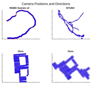
Figure 4.1 – Visualization of camera locations (red) and viewing directions (blue) from our collections (bottom) and previous datasets (top). We collect densely sampled RGB-D images of scenes for use in training and benchmarking active vision systems. The dense sampling allows “virtually” moving a camera through a scene. While other datasets do sample multiple images per scene, they often sample either from just a few positions or along only a few paths through the environment (Lai et al. (2014); Silberman et al.
(2012)). Note that the physical scale is different in each plot. . . 27 Figure 4.2 – How sensitive our detection system is to change in camera position. As
the distance between two images of an instance increases(x-axis), the change in detection score(y-axis) tends to increase. Each line represents one in-stance. The vertical blue line shows our chosen sampling resolution of
30cm. . . 28 Figure 4.3 – A comparison between an initial depth image(left) and the improved depth
image(right). The improved depth images allow us to better handle oc-clusion when projecting point cloud labels from the dense reconstruction
to bounding boxes in the RGB images. . . 30 Figure 4.4 – Four dense reconstructions of scenes from our collected data. We label
objects in 3D using the dense reconstructions then project to each cam-era image to obtain 2D bounding boxes. (Reconstruction tool from
Figure 4.5 – Example of how motion is possible through a scene in AVD via our
move-ment pointers. . . 32 Figure 4.6 – Detection scores for four different instances in various scenes. Dots are
camera position, color indicates score. Only cameras that see the instance (purple diamond) are shown. Notice certain viewpoints consistently yield higher scores. It would be advantageous for a robot to move from green
views to red ones. . . 34 Figure 4.7 – Example of how movement affects detection output for a single instance.
The proposed box with highest score> .1for the crystal hot sauce bot-tle instance is shown in each image. Object instance and scene correspond
to the bottom left plot in Figure 4.6 . . . 35 Figure 4.8 – Example paths taken by our active vision system. The arrow indicates
the action chosen by the action network. . . 36 Figure 4.9 – Overall architecture of our active recognition system. It consists of three
components. A CNN for extracting image features from the entire im-age given the current view, an instance classifier for classifying the cropped object, and an action network for selecting the next action in order to
im-prove classification. . . 38 Figure 4.10 –The relative improvement in classification accuracy for different active
vision policies. As the system makes more virtual moves through the scene(T increases), our method is able to move to a position that increases clas-sification performance. Making random moves, or just moving forward,
does not improve performance much. . . 40 Figure 4.11 –Example “target images”. . . 43 Figure 4.12 –Some examples of labeled images. . . 44 Figure 4.13 –Camera locations (red) and directions (blue) from AVD scenes. The dense
sampling of images allows benchmarking active navigation tasks using
visual input. . . 45 Figure 4.14 –Camera locations (red) and directions (blue) from AVD scenes. The dense
sampling of images allows benchmarking active navigation tasks using
visual input. . . 45
Figure 5.1 – Example of target images (front and back view of the object), and an in-put “scene image” that contains the target object in a different pose, par-tially occluded, at small scale. The object’s bounding box (in red) is
Figure 5.2 – The proposed architecture. The bottom box represents the RPN stage of Faster R-CNN. The top box is our TDID-RPN model. We enrich the fea-ture representation with a joint embedding for scene-target pair. TDID first extracts features from scene and target image (feature extractor weights are shared), then combines those with a novel TDID-RPN embedding module, and finally applies the detection prediction head. The detailed structure of the TDID-RPN embedding module is shown in Figure 5.3
and described in Section 5.2. . . 49 Figure 5.3 – TDID-RPN embedding: given scene (gray) features, and a set of target
(red) features, makes a joint tensor embedding. Target features are pooled across all views and then depth-wise correlated with (*) and subtracted from (-) scene features. In final model scene features (IMG in Table 5.1, dotted line and white box in this figure) are not used. Features for three target images are shown, but in general any number of views can be used.
. . . 50 Figure 5.4 – Visualization of the CC and DIFF features. The images are1xC, where
C is the number of feature channels, picked from a random location of the respective feature map. TheCC features give sparse but clear sig-nals of presence or absence of certain features. DIF F feature provide more complex information, complementing the sparsity of theCC fea-tures. Note the images are not at the same scale for easier visualization, theCC features have much higher raw values than theDIF F features
by the nature of the operations. . . 52 Figure 5.5 – TDID Box Detection Head (BDH) architecture. For each target image,
first pool to a2x2region of interest, then stack along the feature dimen-sion. Compute the cross correlation as in the RPN module, but for each view individually. Then max-pool over all views. Convolution layers for class prediction and bounding box regression not shown. In general any
number of target views can be inputted. . . 54 Figure 5.6 – Example target images. . . 62 Figure 5.7 – From Left: target images, scene image, VGG activations, our joint
rep-resentation activations. The top row shows an example where the target was used in the train set, bottom row shows a novel target. The model was successful in detection both objects. Ground truth bounding box in
Figure 6.1 – Default Box Predictions. At each of a fixed set of locations, indicated by solid boxes, predictions are made for a collection of “default” boxes of different aspect ratios. In the SSD detector, for each default box a score for each object categery (Conf) is predicted, as is an offset in the posi-tioning of the box (Loc). This work adds a prediction for the pose of an object in the default box, represented by one of a fixed set of possible poses,
P1. . . Pn. . . 67 Figure 6.2 – Two-stage vs. Proposed.(a) The two-stage approach separates the
de-tection and pose estimation steps. After object dede-tection, the detected ob-jects are cropped and then processed by a separate network for pose es-timation. This requires re-sampling the image at least three times: once for region proposals, once for detection, and once for pose estimation. (b) The proposed method, in contrast, requires no re-sampling of the im-age and instead relies on convolutions for detecting the object and its pose in a single forward pass. This offers a large speed up because the image is not re-sampled, and computation for detection and pose estimation is
shared. . . 68 Figure 6.3 – Our Model Architecture. Detection and pose estimation network for
the “Share 300” model that shares a single pose prediction across all cat-egories at each location and resizes images to 300x300 before using them as input to the network. Feature maps are added in place of the final lay-ers of a VGG-16 network and small convolutional filtlay-ers produce esti-mates for class, pose, and bounding box offsets that are processed through non-max suppression to make the final detections and pose estimates. Red
indicates additions to the architecture of SSD (Liu et al. (2016)) . . . 69 Figure 6.4 – Pascal 3D+ Qualitative Results. Results on 8 bin detection and pose
estimation on the Pascal 3D+ dataset. Each image has a corresponding detection class confidence, pose confidence, predicted pose label, and ground truth pose label, respectively. Columns one and two show cor-rect pose predictions with high and low detection scores; column three shows pose predictions that are off by one bin; and column four shows
some difficult examples where our system fails. . . 78 Figure 6.5 – Method overview: The generator, composed of both a pose regressor and
a non differentiable renderer, makes a 3D pose prediction and renders the predetermined object at the predicted pose. The discriminator scores how visually similar the poses depicted in the images are. This score is
Figure 6.7 – Examples of ‘symmetric’ objects in the T-LESS (Hodaˇn et al. (2017)) dataset. The symmetries range from mostly identical (a), to shape but not texture (b), to very small texture differences (c). This can lead to
am-biguities when trying to label data or train a pose estimator. . . 82
Figure 6.8 – Garchitecture. . . 83
Figure 6.9 – Darchitecture. . . 84
Figure 6.10 –Dtraining input. . . 85
Figure 6.11 –Generating a ’fake‘ training pair forD. . . 86
Figure 6.12 –Output fromDfor 2D square with reference pose of20°. . . 87
Figure 6.13 –Possible training technique forG. . . 87
Figure 6.14 –Estimating the gradient for trainingG. . . 89
Figure 6.15 –How we use the output surface of the discriminator to estimate a gradi-ent for training the pose prediction network. . . 89
Figure 6.16 –Inputs (first column), outputs from generator (second column), and out-puts from discriminator (third column) for our experiments on 2D shapes. . . . 92
Figure 6.17 –Overview for training the discriminator, training ‘fake’ images are gen-erated using the generator and shown in dark orange, whereas training ‘real’ images is depicted in dark blue. . . 93
Figure 6.18 –Overview for training the generator 1) we generate a pose, and 2) we sam-ple multisam-ple perturbed poses to find the most valuable as target training. . . . 95
Figure 6.19 –How different models’ (SymGAN, our baseline) output change as an ob-ject is rotated in a plane (approximately). The arrow depicts the orien-tation of the example image in the center, the object is then rotated 360 degrees around an axis coming out of the page, and the models’ 3D pose outputs are project to a plane and plotted. GT means ground truth pose. . . . 100
Figure 6.21 –Qualitative results of our viewpoint predictor on scene 1 from T-LESS dataset. The scene is composed of object id. 02, 25, 29, and 30 shown
LIST OF ABBREVIATIONS
CNN Convolutional Neural Network
R-CNN Region Convolutional Neural Network GAN Generative Adversarial Network
GT Ground Truth
CHAPTER 1: INTRODUCTION
Humans can use visual input as a rich source of information for interacting with their environ-ment. The ubiquity of cameras in modern society have made them a cheap and readily available sensor, enabling robots to make use of perception as well. There is a long way to go, however, from capturing images with cameras to using that data to inform a robot’s actions. Enter com-puter vision. A broad field, comcom-puter vision studies how to solve problems like understanding underlying geometry—distance or location of observed entities—higher-level semantic informa-tion, such as what objects are present.
Object recognition involves identifying objects in images and videos. This includes the pop-ular tasks of image classification, object detection, and segmentation. There are many problems in robotics that are obvious applications of object recognition work, in industrial settings such as the Amazon Picking Challenge, autonomous cars, and assistive robots in the home (Zeng et al. (2018); Wang and Wong (2019); Geiger et al. (2013)). Most robots outside of extremely struc-tured assembly line environments could make use of computer vision and object recognition to better understand and interact with the world.
Image classification in particular has been a driving force behind many of the recent advances in computer vision. Krizhevsky et al. (2012) revolutionized the recognition field, and computer vision in general, with their deep-learning based AlexNet submission to the ImageNet Challenge (Russakovsky et al. (2015)). AlexNet significantly outperformed other methods and in recent years neural networks, in particularly convolutional neural networks (CNNs), have been a part of state-of-the-art methods for most object recognition tasks.
large and complex environment, breaking down which objects are where can be an important step in performing successful actions. Girshick (2015) designed the Faster R-CNN object detector, built on top of other region based CNN (R-CNN) detectors and other works on classification. The general pipeline is to first detect where objects are in an image, and then for each possible object identify its type. Recent methods have combined both steps in one, (Redmon et al. (2016); Liu et al. (2016)) improving speed but sacrificing some accuracy. The speed/accuracy trade-off is especially interesting in robotics where the vision module will likely be only one part of a complex system expected to run in real-time.
Perhaps more than anything else, besides the advancement of specialized hardware like the GPU, large datasets have enabled the application and development of deep-learning and neu-ral networks for computer vision tasks. Russakovsky et al. (2015) created ImageNet, the first large scale dataset for image classification containing over 1 million images. Everingham et al. (2012) and Lin et al. (2014a) collected and released the PASCAL and MSCOCO object detection datasets respectively, containing tens of thousands of images, enabling research on using CNNs for object detection. These deep-learning scale datasets usually focus on labeling objects into a fixed set of general categories such as chair or bottle. This is very useful for many applications and general computer vision research, but often robots find themselves in more specific situations. A robot set in a factory or a home will have a relatively small set of distinct individual objects it interacts with. It is likely important to discriminate between a dining chair and an office chair, or a bottle of water vs. a bottle of soda, or even a bottle of Pepsi vs. a bottle of Coke. New cat-egories might also be introduced frequently, when a new product is introduced at the factory or a new brand of cereal is brought home from the grocery store. Song et al. (2015) envision a sce-nario where a robot lives in a home and sends images of new objects brought home to the cloud to be annotated. To enable these kinds of functionalities, we need datasets more suited to robotics applications.
to complete its task, and so a system must be able to use visual input to inform the robot’s ac-tions. The robot also has thecapacityto move, and so a system may be able to use movement to improve its visual understanding of the environment, for example moving around an occluding object. A major roadblock of introducing motion in a research setting is the difficulty of repro-ducing work done on a robot in the real world. It is usually impossible to duplicate the exact experimental environment in different locations, not least because of simple factors like lighting changes.
Once a robot recognizes an object, and possibly moves to it, more information is required for the robot to have a successful interaction. Object pose, a measure of the location and ori-entation of an object in 3D space, can be useful for multiple downstream robotic tasks such as grasping. Hodan et al. (2018) organize a benchmark on estimating object pose on objects rele-vant to robotics applications. Many recent techniques have advanced the state-of-the-art using deep-learning techniques (Xiang et al. (2018); Sundermeyer et al. (2018); Deng et al. (2019). An inherent issue of all pose estimation work is the ambiguity of object symmetries. Two views of an object, two visual inputs to a system, can be identical but have different labels for pose. Find-ing a robust and elegant solution to this problem is an important component of a robotic vision pipeline.
In this work we build computer vision tools useful to specific applications in robotics. We start with data that enables research on a variety of robotic tasks. This includes simulation of motion in a reproducible way usingreal imagesin real environments. General object detection methods are then extended to improve performance on fine-grained (individual) object instances. Once these objects are detected, we design a robust training algorithm for deep-learning pose estimation methods that elegantly handles object symmetries. We detail each contribution below.
1.1 Thesis Statement
1.2 Outline of Contributions
This thesis contributes to the intersection of computer vision and robotics communities with the following works:
A dataset for active vision and fine-grained object instances. We build a dataset with two goals in mind: enabling the simulation of motion using real imagery, and deep-learning scale examples of fine-grained object instances for object detection (Ammirato et al. (2017)). Using a robot mounted with a Kinect v2 sensor, we capture data in a regular pattern in indoor environ-ments, placing a consistent set of grocery store objects in each scene. Using 3D computer vision techniques, we are able to expedite the labeling process, avoiding crowd-sourcing and producing high quality labels. We show our capture method is useful for simulation of motion for object recognition, and that we can learn to improve recognition using active vision.
2D Object Detection for Fine-Grained Object Instances. Using the newly available data, we design a new object detection method for fine-grained object instances. We adapt methods like Faster R-CNN (Ren et al. (2015)) designed for general objects, taking advantage of the speci-ficity of our problem to improve accuracy. In addition to classic object detection on a fixed set of objects, the ability to recognize new types of objects is of great interest to robotics. We apply our method to multiple few-shot recognition tasks, recognizing objects from few examples without retraining our system at all. Our Target Driven Instance Detection method shows state-of-the-art results on a variety of object detection tasks.
Pose Estimation and DetectionWe first design a method to combine object detection with pose estimation into a singular efficient framework, keeping in mind the restraints of robotic sys-tems in terms of computational resources and time (Poirson et al. (2016)). Our method employs a binning technique, where we discretize the pose space into coarse intervals (bins), leading to a less accurate but simpler and faster system. We see our method as a useful first step towards solving the pose problem with deep-learning techniques, as well as an effective pre-processing tool to enable a finer-grained pose estimation downstream.
CHAPTER 2: TECHNICAL INTRODUCTION
Computer Vision is a diverse and popular field with many sub-problems studied by many researchers. We first will define some of these sub-problems, and a few other terms, so their use is clear in the remainder of the text. Following these definitions we will delve into some technical details behind deep-learning techniques for object recognition.
2.1 Task Definitions
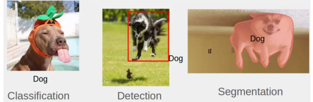
Object ClassificationObject classification is the task of assigning single labels to an image. Usually the input is a cropped image so that there is one foreground object visible, and the output is a label for that image. See the left column of Figure 2.1.
Object DetectionObject detection can be thought of as object classification, plus localization. The input is an image, containing any number of objects at any scale, and the output is a set of bounding boxes. Each bounding box defines a region in the image, and also gives a label to indicate the class (or type) of object in the box. There is work on both 2D object detection, where the bounding box is defined only in the image plane, and 3D object detection, where the bounding box attempts to define the object’s full location in 3D space. In this work, we focus
solely on 2D object detection, and so will refer to it simply as (object) detection. See the middle column of Figure 2.1 for an example input image and bounding box output for the ‘dog’ class.
Object SegmentationObject segmentation is similar to object detection but outputs a finer grained labeling of the image. The input is the same as in detection, but the output is a class label for every pixel of the input image. See the right column of Figure 2.1 for an example. In this case, the pixels on the dog are labeled as being in the ‘dog’ class, and every other pixel is ‘background’. A very important and interesting problem in computer vision, segmentation is not covered in this thesis.
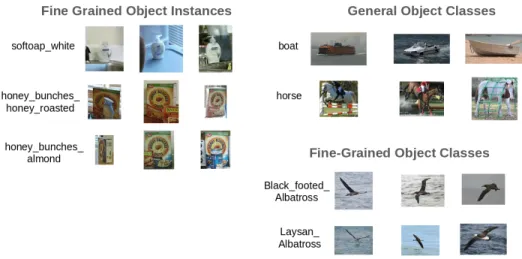
Fine Grained Object InstancesIn object recognition, there are many terms for describing the classes of objects being recognized. We are particularly interested in two attributes classes of objects can have: intra-class variation and inter-class variation. Arguably the most popular tasks, like ImageNet classification or MSCOCO detection, operate on what we callgeneral object categorieswith large intra-class variation and large inter-class variation. This usually includes classes like boat, person, cow, etc. Fine-Grained Visual Categorizationis another popular task, in which the classes have small inter-class variation, but there is not much restriction on intra-class variation. A relatively newly popular task,instance segmentation, requires systems to segment objects from general object categories, but also distinguish between each occurrence of each ob-ject category. An instance segmentation input may be an image with three boats visible, and the goal would be to label each boat as belonging to the general ‘boat’ class, as well as an identifier distinguishing which boat is which. So the system may output labels for ’boat-1‘, ‘boat-2’, and ‘boat-3’. The term‘instance’is also used in many classic computer vision and robotics works to
describe classes of objects with little to no intra-class variation. We definefine-grained object instancessimilarly to the classic definition of instances, but add the fine-grained descriptor to distinguish frominstance segmentation, and to indicate that in many cases there is very small inter-class variation. See Figure 2.2 for examples of each term.
Figure 2.2: Examples of a fine-grained object instances, general object categories, and general fine-grained classes. Images from Ammirato et al. (2017); Everingham et al. (2012); Wah et al. (2011).
We define the full object pose as the six degrees of freedom pose of an object in space, in-cluding 3D translation (x,y,z position) and 3D orientation (roll, pitch, yaw angles). A variety of work has studied different parts of this problem. Object detection only deals with the two trans-lation parameters in the image plane, and ignores the third transtrans-lation parameter and orientation. Depth estimation methods output the third out-of-plane translation parameter. Many recent works have focused on the full 6D problem, as we will discuss below, and some focus only on the 3D orientation.
Active Vision
Active Vision, not to be confused with Active Learning, is a broad set of problems where the system has control to move the camera, in a closed loop. This includes tasks such as moving to the next best view to improve recognition, or actively searching for objects in an environment.
2.2 Neural Networks
Figure 2.3: Example basic neural networks.
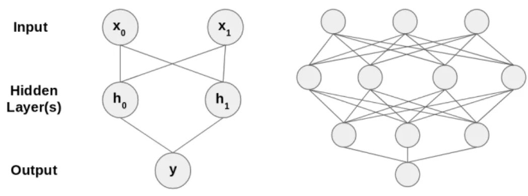
2.2.1 Basic Overview of a Training Simple Net
See Figure 2.3 for two examples of simple fully connected feed forward neural nets. On the left example,{x0, x1}are the scalar inputs,{h0, h1}are the feature values in the ‘hidden’ layer, andyis the final output. Each edge in the graph represents a scalar weight,w, and each collection of edges between nodes forms a ‘layer’,l. We apply the weights as follows:
hlj =X i
(wi,jl ) +blj
wherewl
i,j connectsh l−1
i andhlj andblj is a scalar bias term. In Figure 2.3 the inputs are at layerl = 0, and the output is at layerl = 1. Our goal is to train the weights to produce the de-sired output given some input values. In supervised learning, which is the focus of this thesis, we make use of ground truth labelsyGT. Using the ground truth target we can compute a met-ric, scoring how close the networks output is the GT, commonly called a loss function, denoted
L(y, yGT).
Ideally we would like to change the weights to minimize the loss function, but it is not im-mediately clear how to accomplish this. If, however, our loss function is differentiable, we can easily find how to change the output value to lower the loss by moving in the direction of the gradient, ∂L∂y. Now consider a weight in the output layer,w10,0, that connects{h0, y}in Figure 2.3. We would like to find ∂w∂L1
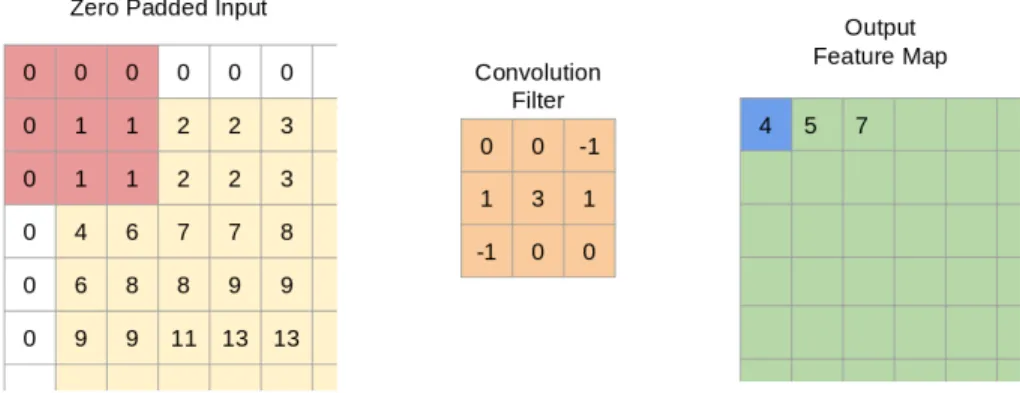
Figure 2.4: Example application of a convolution filter. The input is first padded with zeros (for convenience) and then the filter is applied to each location to form the output feature map.
∂L ∂w1 0,0
= ∂y
∂w1 0,0
· ∂L
∂y =h
1 1 ·
∂L ∂y
We can continue using chain rule to push the gradient back through every layer of the net-work, getting equations for how to update every weight and bias. In practice neural nets will also make use of non-linear activation functions after applying the weights, but these functions can be seamlessly incorporated into back-propagation as long as they are differentiable. An optimiza-tion technique such as stochastic gradient descent (SGD) or the Adam optimizer (Kingma and Ba (2014)) is used to make small updates in the gradient direction in an iterative fashion, as the inputs to the network cycle through the training dataset.
The requirement that each element of a network be differentiable is an integral requirement for back-propagation. This will become important when we look at training our SymGAN pose estimation technique later.
2.2.2 Convolutional Neural Networks
2.4 for an example of applying a filter to an input. In practice the input is often padded with zeros around the boarders so the output is of the same size, but this is not strictly necessary. The convolution filter is applied centered at each location of the input, in Figure 2.4 we see it centered on the top-leftmost entry. We get a value in the output from the equation:
Oi,j = m=2 X 0
n=2 X 0
Ii−m−1,j−n−1∗fm,n
Where{i, j}are indices into the input,I, and{m, n}or indices into the convolution filter,f. This operation produces what is referred to as afeature map,O, where each element inOis a featureextracted by the filter. These features could represent things likes the presence of edges or blobs of color, or higher-level concepts like the presence of eyes or legs, or things that are not easily interpreted by humans but useful for the network.
Though the example above maintains spatial dimensions when extracting a feature map from an input, in practice CNNs require some method of down-sampling to reduce the feature map resolution. Generally it is useful to expand the channel dimension, or number of features (filters), to get a better semantic representation of the image, and reduce the spatial dimension for effi-ciency. This down-sampling can be accomplished with convolution filters, namely by increasing thestride, but is most commonly implemented with pooling layers. These layers behave similarly to a convolution filter, moving in a sliding window fashion over an input feature map.
2.3 Object Detection
Figure 2.5: Visualization of anchor boxes.
Faster R-CNN is often referred to as a two-stage object detector, though for our discussion we will consider three steps. Feature extraction via a backbone network is step zero, converting the input image to a feature map. Region proposals are generated as step one, via a hand-crafted method like Selective Search (Uijlings et al. (2013)) in older methods, Faster R-CNN uses a learned Region Proposal Network (RPN) . The region proposal outputs a set of ROIs (regions of interest), locations in the image that are likely objects. The ROIs can be pooled to a common size, resembling classification-style inputs, and then processed by the second-stage network. Generally this is done at the feature level, after the backbone feature extraction. So the inputs to the second stage are not crops from the original input image, but are instead crops of the extracted feature map from step zero. The second-stage network classifies each ROI into one of the pre-defined set of classes, or background, and outputs location parameters to refine the bounding box location of the ROI in the original input image.
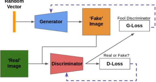
Figure 2.6: Overview of GAN for image generation. Solid lines indicate forward pass, dashed lines where the loss is back-propagated.
of three anchor boxes overlaid on one location of a feature map. The RPN classifies each box as object or background, and predicts offsets for modifying the bounding box defined by the anchor boxes scale, aspect ratio, and location in the feature map. At training time each anchor box is matched to a ground truth box if it has high intersection over union (IOU), or to background otherwise.
2.4 Generative Adverserial Networks
GANs Goodfellow et al. (2014) have become a popular technique for a variety of tasks. The method was originally used for image generation (Zhu et al. (2017a); Wang et al. (2018)) but since has been applied to new domains such as reinforcement learning (Ho and Ermon (2016)). Our work, SymGAN, uses the GAN framework for object pose estimation. We can, however, gain useful intuition about the GANs from understanding the original image generation applica-tion.
control the content of the output image (Mirza and Osindero (2014)) but that is outside the scope of this discussion. The goal of the discriminator is to classify an input image as either ‘real’ or ‘fake’. Fake images are those output by the generator, and real images are sampled from some
dataset of actual images from a camera, such as ImageNet. The discriminator loss, D-Loss in Figure 2.6, is usually a simple classification loss such as cross entropy, though other work has explored other methods to stabilize training Arjovsky et al. (2017). The generator loss, G-Loss, is essentially the inverse of D-Loss on the fake images. Intuitively the generator is trying to fool the discriminator by generating images that look as if they come from the the real image distribu-tion. More formally, from Goodfellow et al. (2014), the generator,Gand discriminator,D, play a minimax game with value functionV:
min
G maxD V(G, D) =Ex∼pdata(x)[logD(x)] +Ez∼pz(z)[log(1−D(G(z)))]
CHAPTER 3: RELATED WORKS
We now explore many related works on a variety of topics relevant to this thesis.
3.1 Datasets in Computer Vision
General Object CategoriesThe datasets that have been a driving force in pushing the deep learning revolution in object recognition, Pascal VOC (Everingham et al. (2010)), the ImageNet Challenge (Russakovsky et al. (2015)) , and MS COCO (Lin et al. (2014b)) are all collected from web images (usually from Flickr) using web search based on keywords. These image collections introduce biases from the human photographer, the human tagging, and the web search engine. As a result objects are usually of medium to large size in images and are usually frontal views with small amounts of occlusion. In addition these datasets focus on general object category recognition. The state of the art for object classification and recognition in these datasets is based on either object proposals and feature pooling following (Uijlings et al. (2013)) with advanced deep networks (Girshick et al. (2014); He et al. (2016)) or on fully convolutional networks imple-menting a modern take on sliding windows (Liu et al. (2016); Redmon et al. (2016); Poirson et al. (2016)) that provide frame-rate or faster performance on high-end hardware for some reduction in accuracy.
There are many RGB-D datasets available today, but none with a focus on simulating robotic motion through an environment, or with deep-learning scale real-world examples of fine-grained object instances. Firman (2016) gives a fairly comprehensive list of various RGB-D datasets, including some that focus on fine-grained object instances. We categorize these datasets into two sets: ‘table-top’ data and ‘scene-focused’ data. Singh et al. (2014); Lai et al. (2011) are two pop-ular examples of ‘table-top’ style data. This type of data, especially the data in BigBIRD (Singh et al. (2014)), is similar to what manufactures may provide for robots in the future. BigBIRD consists of 125 objects, each placed on a turn-table with a plain white background. Each object is then rotated 360°, stopping every three degrees to capture photos from five different elevations, resulting in six-hundred images per object. Lai et al. (2011) perform a similar capture procedure, gathering data for 300 fine-grained object instances. While not capturing real-world scenes, the number of views and detail for each instance in this data can provide valuable training data for instance recognition systems.
‘Scene-focused’ datasets (Silberman et al. (2012), S. et al. (2015),Lai et al. (2014), and Geor-gakis et al. (2016)) do explore environments beyond ‘table-top’ data but do not have a dense set of views to simulate robot motion and can often be simple/staged compared to real-world scenes. These data-sets often have only one or two paths through the scene. An actual robot in the real-world has many choices of where to move, and the controller has to be able to pick a good path.
3.1.1 Object Pose Datasets
3.1.2 Active Focused Datasets
There has been a recent influx of datasets focusing on active vision tasks, where visual ob-servations are considered jointly with some control/action authority. The existing datasets vary in the level of visual realism they provide, their scale, the type of modalities they can simulate and ability of agents to interact in the world. They can be broadly partitioned into CG synthetic worlds derived from the original SUNCG (Song et al. (2017)) dataset or datasets derived from scans of the real world (Chang et al. (2017)).
Matterport3D (Chang et al. (2017)) is a large-scale RGB-D dataset containing 10,800 panoramic views about 1-1.5m apart with surface reconstructions, camera poses, and 2D and 3D semantic segmentation annotations. The scale and visual realism of the data is impressive, but the poses where high resolution panoramas are available are quite sparse. Views generated outside of the panorama grid are obtained by rendering mesh reconstructions and have notable artifacts.
The MINOS (Savva et al. (2017)) environment is a synthetic environment which contains both synthetic scenes from SUNCG (with over 45,000 scenes) and meshes of reconstructed scenes from the Matterport3D dataset (with 90 multi-floor houses). While the scale of the dataset is appealing, the quality of the visual observations is limited to either synthetic renderings of SUNCG scenes or renderings of reconstructed meshes, which suffer from many reconstruction artifacts affecting the visual observations. Additional sensing modalities of depth, plane normals and semantic segmentation and capability of arbitrary viewpoints and continuous motion are enabled by the dataset. House3D (Wu et al. (2017)) is also a fully simulated large scale environ-ment derived from SUNCG and enables visual observations as rendered views along with depth and semantic segmentation.
Efforts to eliminate some of the reconstruction artifacts have been tackled recently by Xia et al. (2018), using a novel image-based rendering approach to eliminate some of the visual arti-facts. The resulting rendered views while free of some artifacts are still quite blurry.
The API for this environment does not provide access to other modalities and the initial scale of the environments is smaller than other synthetic datasets (2-3 bedroom houses compared to multi-story buildings provided by Matterport3D and SUNCG). Another effort at a simulated world is from Weichao Qiu (2017).
The tasks studied in the context of these datasets and environments include navigation (Gupta et al. (2017)), target driven navigation (Zhu et al. (2017b)), visual question answering (Das et al. (2017)), and planning (Anderson et al. (2017)). While it can make sense to study each of these in both completely artificial environments as well as real scenes, using real imagery allows probing aspects of visual perception that might over-fit or otherwise yield unrealistic performance on CG data.
3.2 Object Classification
3.3 Object Detection
Pre-Deep LearningTraditional methods for object detection in cluttered scenes follow the sliding window based pipelines using hand crafted features such as HOG (histogram of gradients) (Dalal and Triggs (2005)). Efficient methods for feature computation and classifier evaluation were developed such as Deformable Parts Model (DPM) (Felzenszwalb et al. (2010)). Examples of using these models in the table top setting include (Lai et al. (2011); Song et al. (2012)). Ob-ject detection and recognition systems that deal with textured household obOb-jects such as Collet et al. (2011) and Tang et al. (2012) take advantage of the discriminative nature of local descrip-tors. A disadvantage of these local descriptors is that they usually perform poorly in the presence of non-textured objects. Some of these issues were tackled by Hinterstoisser et al. (2011) which used template based methods to deal with such texture-less objects. Hand engineered features typically work well in table top settings that contain a relatively small number of objects at rela-tively large scale (Zeng et al. (2018)).
Deep LearningState-of-the-art object category detectors have been improved significantly over the last few years in both accuracy and speed. These detectors generally rely on a backbone architecture, such as the popular classification networks VGG (Simonyan and Zisserman (2015)) or ResNet (He et al. (2016)), to extract features from the image and then add a detection module on top of these features.
Two-stage detectors, such as the R-CNN family of detectors (Girshick et al. (2014); Girshick (2015); Ren et al. (2015); He et al. (2017)), and R-FCN (Dai et al. (2016)), rely on an initial region proposal method followed by a classification and location regression of the proposed regions.
et al. (2017); Shrivastava et al. (2016)), which can borrow rich semantic information from deeper layers and improve in accuracy for small objects, though usually at reduced speed.
Deep Learning and Fine-Grained Instance DetectionClassic approaches to detecting fine-grained object instances often attempt to match low-level hand-crafted features such as SIFT (Lowe (2004)), in a sliding window manner. Applying deep learning to fine-grained object in-stances is often a challenge due to the limited amount of training data. The recent release of the AVD, a contribution of this thesis, and the GMU Kitchens dataset has mitigated this somewhat, but there is still a gap in scale between instance datasets and those for general object categories.
Dwibedi et al. (2017); Georgakis et al. (2017) attack the problem of limited training exam-ples by synthesizing new examexam-ples with different background images, enabling the use of deep-learning based detectors. In both of these works general object category detectors such as SSD (Liu et al. (2016)) or Faster R-CNN (Ren et al. (2015)) are still used to solve the instance detec-tion problem. One contribudetec-tion of this thesis is to build a detector using CNNs that is tailored specifically to the fine-grained instance detection problem.
3.4 Tracking
The tracking problem is, in one popular formulation, related to object detection, in particular fine-grained object instance detection. Given an initial bounding box of an object, one tracking task is to localize (detect) the same object appearing in each subsequent video frame. Most recent approaches in tracking attempt to compute some similarity measure between the target object crop and a patch in the current query frame, (Bertinetto et al. (2016a) Henriques et al. (2015) Danelljan et al. (2014)). Held et al. (2016a) combine the features of crops from previous and current frames to regress the location directly. Valmadre et al. (2017) interpret the correlation filter learner as a differentiable layer and enables learning deep features that are tightly coupled to the correlation filter.
Siamese network to be fully convolutional. There have been a recent line of Siamese RPN style networks for tracking released (Li et al. (2018a); Zhu et al. (2018); Wang et al. (2019); Zhang et al. (2019); Bo et al. (2019)) that are similar to a contribution of this thesis, Target Driven In-stance Detection, though have important differences. Strong priors on the appearance and loca-tion of target object and background exist in tracking, namely that neither changes much frame to frame. These priors include scale, location, illumination, orientation and viewpoint. The fine-grained object instance detection setting requires robustness to larger changes between target and query image.
3.5 Object Pose Estimation
Object pose estimation is a popular problem in the robotics and computer vision communi-ties, and usually consists of 3D localization and 3D orientation estimates to form a full 6D pose. This problem has been addressed by many works using classic computer vision algorithms, such as Hinterstoisser et al. (2012); Wohlhart and Lepetit (2015). Pauwels et al. (2016); Tjaden et al. (2017) use forms of template or feature matching. Tan et al. (2017); Brachmann et al. (2016, 2014) have applied classic machine learning techniques. Wohlhart and Lepetit (2015) introduce an effective approach to feature learning for simultaneous categorization and pose estimation for single objects on uniform backgrounds. Recently many works using deep learning and convo-lution neural networks (CNN) have been proposed (Kehl et al. (2017); Mousavian et al. (2017); Xiang et al. (2018); Tremblay et al. (2018c); Manhardt et al. (2018); Tekin et al. (2018)).
Most of these methods need specific handling for symmetrical objects, such as special la-belling (Tremblay et al. (2018b)). Kehl et al. (2017) added a classifier for pseudo symmetric objects, but it still requires hand labeling information about the object . Xiang et al. (2018) de-fined a loss function similar to the average distance metric (ADI) . This approach excels under objects with very symmetrical shape, the metric matches each point on the 3D model in the pre-dicted pose with the closest point on from the ground truth pose. Hodan et al. (2016) showed that using ADI can break under self-occlusion, when the object looks symmetric in two views but some hidden part has moved,e.g., the handle of a mug . Moreover the loss does not take into ac-count visual queues,e.g.,given an object that is visually dissimilar, but the shape does not change such as a texture cylinder would get label as symmetrical under the ADI loss.
Sundermeyer et al. (2018) implicitly learn a representation from rendered 3D model views us-ing an auto-encoder . At test time a crop of the object is encoded and then compared via nearest neighbor search to a dictionary of encoded poses to retrieve the final orientation. Their method is limited by the discretization of the object poses, whereas our is technically continuous and outputs a pose directly.
3.6 Generative Adverserial Networks
3.7 Domain Randomization
Our SymGAN work is also part of a larger effort to accomplish training on simulated data while running inference on real data, this is also known as the reality gap problem. As such our method is trained on rendered images while tested on real images and only necessitates a 3D CAD model of the object of interest, which is often easier to obtain than hand labelling real-world training data. A popular approach to solve this problem is the usage of domain randomiza-tion Tobin et al. (2017); Tremblay et al. (2018a) as an inexpensive method to bridge that gap.
This method consists of training a model with extreme visual variety so that when presented with a real-world image the model treats it as another visual variation. It has been successfully applied – though usually needing fine tuning or more structure in the randomization to achieve state of the art results (Prakash et al. (2019); Tremblay et al. (2018c)) – to car detection (Trem-blay et al. (2018a); Prakash et al. (2019)), pose detection (Trem(Trem-blay et al. (2018c); Sundermeyer et al. (2018)), vision based robotics manipulation (Tobin et al. (2017); Tremblay et al. (2018b); James et al. (2017)), robotics control (Chebotar et al. (2018); Tan et al. (2018)), and more.
3.8 Active Vision
Active vision has a long history in robotics. Early work largely centered around view se-lection (Bajcsy (1988); Jia et al. (2011)). Others (Karasev et al. (2012); Atanasov et al. (2013); Velez et al. (2012)) have worked on the problem from a more theoretical perspective, but under many simplified settings for possible motions, or assumptions about known object models. Newer methods have investigated learning how to look around a scene (Jayaraman and Grauman (2018, 2016)).
images (Doumanoglou et al. (2016)). CAD models produce encouraging results, but leave out some real-world challenges in perception.
Doumanoglou et al. (2016) gives a system for object detection, pose estimation, and next best view prediction. They are able to test their detection and pose estimation system on existing real image datasets, but need to collect their own data to test their active vision framework. They collect a small scale dataset of only “table-top” style scenes with about 30-60 images each. This shows the need for a dataset for active vision, while also showing how difficult it can be to collect such data at a large scale.
CHAPTER 4: BUILDING A DATASET FOR VISION AND ROBOTICS
4.1 Introduction
The ability to recognize objects is a core functionality for robots operating in everyday human environments. While there has been amazing recent progress in computer vision on object clas-sification and detection, especially with deep models, these lines of work do not address some of the core needs of vision for robotics. Partly this is due to biases in the imagery considered and the fact that these recognition challenges are performed in isolation for each image. In robotic applications, the biases are different and recognition is performed over multiple images, often with active control of the sensing platform (active vision). We attempt to address part of this dis-connect by introducing a new approach to studying active vision for robotics by collecting very dense imagery of scenes in order to allow simulating a robot moving through an environment by sampling appropriate imagery.
The goals are two-fold, toprovide a research and development resource for computer vision
without requiring access to robots for experiments, and toprovide a way to benchmark and com-pare different approaches to active visionwithout the difficulty and expense of evaluating the algorithms on the same physical robotics test-bed.
Given this labeled data we adapt a state-of-the-art fast object category detector (Liu et al. (2016)) based on deep convolutional networks to the task of recognizing specific object instances in the dataset. While most deep-learning approaches have focused on category detection, instance detection can be practically useful for robotics. This distinction between recognizing a category of object, such as chair, versus a specific object, such as a particular 8.4oz Red Bull can is impor-tant. Our results show that the category detection framework can be adapted to instance detection, but does not completely solve the problem.
Where the detection framework has difficulty is in the range of scales, viewing directions, and occlusions present in everyday scenes (e.g. our data) that is different from the biases present in Internet collected datasets. While the detector performs well for large frontal views of objects its performance falls for other views. This is quantified in Section 4.5.1. This view-dependent variation in recognition performance motivates active-vision for object recognition, controlling the sensing platform to acquire imagery that improves recognition accuracy.
Our high-level goals are based on using the pre-collected dense imagery to develop and test active-vision algorithms. To validate this approach we begin by demonstrating that the imagery is sampled densely enough. In particular we care that the results and accuracy of recognition algorithms on samples of the densely collected imagery are close to the results that would be achieved if the robot moved continuously through the environment. This is explored in Section 4.2.
RGBD Scenes v2 NYUD2
Ours Ours
Camera Positions and Directions
Figure 4.1: Visualization of camera locations (red) and viewing directions (blue) from our col-lections (bottom) and previous datasets (top). We collect densely sampled RGB-D images of scenes for use in training and benchmarking active vision systems. The dense sampling allows “virtually” moving a camera through a scene. While other datasets do sample multiple images per
scene, they often sample either from just a few positions or along only a few paths through the environment (Lai et al. (2014); Silberman et al. (2012)). Note that the physical scale is different in each plot.
The collected dataset and labels are available athttp://cs.unc.edu/˜ammirato/
active_vision_dataset_website/, as well as a small toolbox for visualizations and
loading. Before collection of imagery, release forms were signed and collected allowing free and legal access to the collected data.
4.2 Simulating Motion for Robotic Vision
There are many parts of a robotic system that may be impacted by movement, but we are focused on the vision system, in particular object recognition. To find an appropriate sampling resolution for object recognition, we see how a vision system’s output changes as a function of camera movement. We need to find a sampling resolution that can simulate motion but is also practical for data collection purposes.
0 100 200 0
0.5 1
0 100 200
0 0.5 1
0 100 200
0 0.5 1
0 100 200
Distance Between Cameras (cm)
0 0.5 1
Absolute Difference in Detection Score
How detection changes with movement
Figure 4.2: How sensitive our detection system is to change in camera position. As the distance between two images of an instance increases(x-axis), the change in detection score(y-axis) tends to increase. Each line represents one instance. The vertical blue line shows our chosen sampling resolution of 30cm.
instance detector on each image. For each video, we calculate the difference in detection score for each instance in all pairs of images. For example, we take the fourth and tenth frame and plot the difference in score for an instance against the distance the camera moved between frames. We then plot the distance between the images against the difference in detection score, with results from four videos in Figure 4.2.
4.3 Data Collection Process
Our dataset covers a variety of scenes from office buildings and homes, often capturing more than one room. For example a kitchen, living room, and dining room may all be present in one scene. We capture a total of 9 unique scenes, but have a total of 17 scans since some scenes are scanned twice. Each scene has from 696-2,412 images, for a total of 20,916 images and 54,247 bounding boxes. We use the Kinect v2 sensor and code from Wiedemeyer (2015) for collection.
As stated, we aim to be able to simulate robotic motion through each scene with our scans. At first it may seem the best way to do this is to capture video as the camera moves around the scene. However, in order to get more than one view at any given point the camera must be rotated at that point. Itois not possible to visit the infinite number of points in each scene, so a discrete set of points must be chosen. In a video, even if a consistent frame rate and rotation speed are maintained, there will be images in between the points of rotation that still represent only a single view of a position in the scene. This is unnatural for movement. Imagine a robot arriving at a location and being unable to turn in place.
We choose to have the camera visit a set of discrete points throughout the scene in order to provide some consistency among the images and camera positions. A video could still be col-lected at each point of rotation, but this would increase the dataset size unnecessarily. We choose to sample every 30 degrees at each point of rotation, providing substantial overlap between im-ages while keeping the number of imim-ages in each scene manageable.
The set of points our robot visits in each scene is essentially a rectangular grid over the scene. We make our points 30 centimeters apart, and justify this in later experiments. Our scenes have between 58-201 points, which allow many choices of how to move.
from an initial scan, and then is tested on the same scene with moved or new objects, e.g. Song et al. (2015).
Figure 4.3: A comparison between an initial depth image(left) and the improved depth im-age(right). The improved depth images allow us to better handle occlusion when projecting point cloud labels from the dense reconstruction to bounding boxes in the RGB images.
Figure 4.4: Four dense reconstructions of scenes from our collected data. We label objects in 3D using the dense reconstructions then project to each camera image to obtain 2D bounding boxes. (Reconstruction tool from Furukawa and Ponce (2007).)
4.4 Data Labeling Process
We aim to collect 2D bounding boxes of our 33 common instances across all scenes. In ad-dition, we need to provide movement pointers from each image to allow movement through the scene. We provide pointers for rotation clock-wise and counter clock-wise, as well as translation forward, backward, left, and right.
Sch¨onberger et al. (2016)). From the reconstruction we get the camera position and orientation for each image. We don’t use depth information for the reconstruction because our sampling is so dense that we are rarely testing the limits of the RGB system. See Figure 4.1 for example reconstructed camera positions.
Using the camera positions and orientations we are able to calculate the movement pointers that allow navigation through each scene using natural robotic movements.
To label every object instance in each scan, we feed the output of COLMAP into the dense reconstruction system CMVS/PMVS (Furukawa and Ponce (2007); Furukawa et al. (2010)). This gives us a denser point cloud of the scene that makes it easy for humans to recognize objects. We then extract the point cloud of each instance from this dense reconstruction, and are able to get 2D bounding boxes in every image by projecting the point clouds for each object into each image. See Figure 4.4. Given that most of our scans include multiple rooms and lots of clutter, we must account for occlusion or the point clouds will project through walls and occluding ob-jects and give low quality 2D bounding boxes. We are able use the Kinect depth maps with the reconstructed point clouds and camera poses to account for some occlusion, but not all. Some occlusion is missed by the raw depth maps because they are sometimes noisy, giving wrong or no values for reflectiveshiny surfaces, and are not at the same resolution as the RGB images.
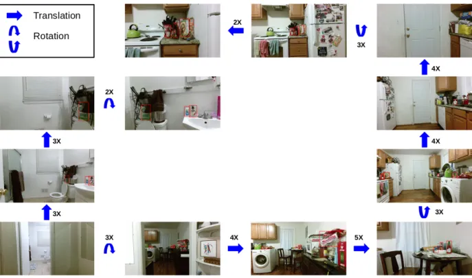
Figure 4.5: Example of how motion is possible through a scene in AVD via our movement pointers.
to fill in any holes of missing values that are left. See Figure 4.3 for a comparison of original to improved depth maps.
Though the improved depths are much better they are still not perfect. There is also noise in the dense reconstruction and noise in the labeled point clouds. Knowing this, we inspect every bounding box ourselves to make sure it contains the correct object, and is not of poor quality (too large or small for the object). We have labeled our scans for BigBIRD objects, yielding an average of over 3000 2D bounding boxes per scan. We provide some measure of difficulty for each bounding box based on its size, leaving adding a measure of occlusion for future work. For our experiments we only consider boxes with a size of at least50x30pixels.
4.5 Detection Performance
Box Size Split 1 Split 2 Split 3
Boxes >100x75 .39 .55 .53
Boxes >50x30 .26 .41 .42
Table 4.1: MAP detection results. Since small boxes are challenging for detection systems to reproduce, we train/test our detector first using only boxes of size at least100x75, and then re-train/test on all boxes at least50x30.
4.5.1 Instance Detection
We use a state-of-the-art class level object detector as a baseline for instance detection on our dataset. We choose the Single Shot Detection (SSD) network from Liu et al. (2016) because it offers both real time detection performance (72 FPS) while maintaining a high-level of accu-racy. This is exciting for robotics applications for which real time performance is crucial. The SSD network consists of a base network, in our case VGG (Simonyan and Zisserman (2015)), with additional feature maps added on top of the base network through a series of 1x1 and 3x3 convolutions.
We separate our dataset into three training and testing splits. Each split consists of eleven scans from seven scenes as training and three scans from two scenes for testing. Since small objects present a particularly difficult challenge for our detector, we first only consider boxes of size at least100x75pixels for training and testing. We then include all boxes of size at least 50x30, adding more training data but also a more difficult test scenario.
4.5.1.1 Qualitative Results
As our data has a wide variety of views of each object, varying pose and scale, we wanted to see how the detector fared with respect to different views. Figure 4.6 shows how detection score changed when camera position changed relative to an object instance. We can see there is a clear pattern showing the detector is more reliable in some camera positions than in others. Figure 4.7 shows how occlusion and object pose can greatly impact the detector even though there are training examples for both cases. We observed similar performance for many objects in all of our test scenes. This behavior motivates an active system that can move from a position with poor detection outputs to one with improved performance.
4.6 How Motion Affects Detection
Figure 4.6: Detection scores for four different instances in various scenes. Dots are camera position, color indicates score. Only cameras that see the instance (purple diamond) are shown. Notice certain viewpoints consistently yield higher scores. It would be advantageous for a robot to move from green views to red ones.
Figure 4.7: Example of how movement affects detection output for a single instance. The pro-posed box with highest score> .1for the crystal hot sauce bottle instance is shown in each image. Object instance and scene correspond to the bottom left plot in Figure 4.6
camera movement. We need to find a sampling resolution that can simulate motion but is also practical for data collection purposes.
We first drive our robot around some scenes, capturing video as if the robot is naturally mov-ing through the environment. We then label all BigBIRD instances in the videos, and run our instance detector on each image. For each video, we calculate the difference in detection score for each instance in all pairs of images. For example, we take the fourth and tenth frame and plot the difference in score for an instance against the distance the camera moved between frames. We plot the results from four videos in Figure 4.2.
Figure 4.8: Example paths taken by our active vision system. The arrow indicates the action chosen by the action network.
4.7 Active Vision Experiments
In this section we propose a baseline for an active instance classification task on our dataset. We envision a scenario where a robotic system is given an area of interest, and the system must classify the object instance at that location. We assume that given an initial area, localizing the same area in subsequent images is straight forward. Based on these assumptions, we propose the following problem setting. As input our agent receives an initial image with a bounding box for the target object. The agent can then choose an action at each timestep and will receive a new image and bounding box corresponding with the action. The goal is for the agent to learn an action policy which will increase the accuracy of the instance classifier.
our dataset contains numerous factors which make the classification task difficult in addition to occlusions, such as varying object scale and lighting conditions. Therefore, we choose to use classification score as the training signal for our active vision system. A new view of an instance can increase both the confidence and accuracy of our classifier. This leads our model to learn a policy which attempts to move the agent to views that improve recognition performance.
As a feature extractor, we used the first 9 convolutional layers of ResNet-18 models (He et al. (2016)), which recently showed compelling results on the 1000 way ImageNET classification task. We used pre-trained models written in the torch framework (Collobert et al. (2011)). The weights for the network are fixed for all experiments although our overall system is end-to-end trainable. The instance classifier and action network share the feature extractor. See Figure 4.9.
We first train an instance classifier for BigBIRD (Singh et al. (2014)) instances, which appear in our dataset. One natural choice might be to train the classifier and action network simultane-ously on our dataset. However, deep neural networks can easily achieve almost 100% classifica-tion accuracy on our training dataset. This type of over-fitting would prevent our acclassifica-tion network from learning a meaningful policy, and does not perform well on the test set.
Thus, we use images from the BigBIRD dataset for training our instance classifier. Even though the BigBIRD dataset provides many viewpoints of an instance, it can’t be directly used for training since it consists of objects against a plain white background. We instead use the provided object masks to crop the object and overlay it on a random background sampled from SUN397 dataset (Xiao et al. (2010); Su et al. (2015b)). In order to prevent our network from over-fitting, we aggressively applied various data augmentations. These included randomly cropping part of the image, performing color jittering, and sampling different lightening. Additionally, since our dataset consists of many small object instances, we randomly scaled the object by a factor ranging from 0.02 to 1.