The rigged monopoly game: Observer's attributions and reactions to unequal allocation of resources

(1)

Mirena Radulova Student number: 0793159

Master’s degree program: Social and Organizational Psychology Supervisor: Riël Vermunt, PhD

Institute of Psychology Leiden Universiteit MASTER THESIS

The Rigged Monopoly Game:

(2)

Abstract

(4)

(5)

1. Introduction

In this demanding era, the issue of unequal allocation of resources is becoming more salient each and every day. The distribution of limited resources exists worldwide in national economies, in courts, in politics and between people. On a broad scale, a resource is a source or supply from which benefit is produced. Foa and Foa (1974) defined a resource as anything that can be transmitted from one person to another. Given the complexity of uniting all resources possible, they further grouped them into six classes: love, status, information, money, goods, and services. In the Resource theory of Social Exchange Foa and Foa categorized: “Money as any coin, currency or token that has some standard unit of exchange value”. Money, however, is the most likely of all resources to retain the same value and meaning regardless of the relation between, or characteristics of, the reinforcing agent, the recipient or observer.” Foa and Foa (1971, p.346349)

Exchange between parties is described as a sequence of resource allocations: allocation of resources by one party is followed by or is simultaneous with allocation of resources by the other. An interaction in which resources are allocated is called an allocation event. An allocation event is instigated by an actor who has power to allocate a resource between himself and other(s) recipients. In addition, the role of the observer has an important role to the situation of the allocation. Observers focus on the allocation decision, on the recipients and on the total event as they maybe affected by the allocation decision. Vermunt, (2014,p.2).

The Observer

(6)

Nisbett research we also know, that actors attribute their actions to situational requirements, whereas observers tend to attribute the same actions to stable personal dispositions (1971, p.80). Furthermore, observers have interpersonal characteristics – beliefs, mood, selfesteem, experience, culture, cognitive style, thoughts, feelings and behaviors that affect perception. In addition, the characteristics that are prominent to this study and that are going to be measured are: their high or low belief in a just world and their attribution style. These characteristics are expected to affect their perception and interpretation when encountered with unequal allocation of resources (see hypotheses). It is therefore, becoming intriguing to understand What is then the observer's reaction to unequal distribution? Or more precisely, what are the reactions when resources are obviously allocated unfairly?

Plan of the study

The question that will be answered in the present study is how observers who read a scenario about an unfair event will attribute success or failure of the fictitious actor, and whether the attribution is dependent or not on characteristics of the event (winning/losing) and/or characteristics of the observer (BJW).

Attributions – External/Internal Locus of Control

(7)

are external factors that are hardly under control of the actor. Stable causes are assigned to ability and task difficulty, whereas the unstable are effort and luck.

BJW

The belief in a just world (BJW) concept is another wellknown model “where just world beliefs act as a perceptual bias in which individuals maintain a belief in a universal justice, even when evidence to that effect is lacking” (Cropanzano & Mitchell, 2005, p.877). Lerner, (1980, p.14) in his research on the “just world” perceptions has proposed, that individuals have a need to believe that they live in a just world; they believe in a world where people get what they deserve and where people deserve what they get. Individuals believe, for instance, that those among us who work hard or who perform good acts obtain rewards for their actions, while the sinners and the laggards receive punishments instead. Similarly, individuals want to believe that positive outcomes, whether money, success or happiness, are obtained only by good people and conversely, that negative outcomes only happen to bad persons. This belief in a just world is invoked by Lerner as a possible explanation for our society's willingness to tolerate the suffering of many disadvantaged individuals (Lerner, 1970, Lerner & Matthews, 1967; Lerner & Simmons, 1966). The operation of system justification motive is consistent with the psychological assumption that people want to believe in a just world (e.g., Hafer & Begue, 2005; Kluegel and Smith, 1986; Major et al 2003). These beliefs are passed from parents to children, from media specifically, or from one's social economic status. The more people favor members of higher status groups over lower status groups (e.g. Jost, Pelham, & Carvallo, 2002) and blame members of lower status groups for their relative disadvantage, the deeper these beliefs are going to be incorporated. (Cozzarelli, Wilkinson, & Tagler, 2001; Crandall, 1994; Katz & Hass, 1988). One of many examples for instance, is the study of McCoy and Major (2006), which proved the hypothesis that activating meritocracy beliefs increases the extend to which individuals justify status inequalities, even when those inequalities are disadvantageous to themselves.

The Rigged Monopoly Game: winning and losing

(8)

Paul Piff (2012, 2014 in press). The results of his sets of experiments in the study “Does money make you mean?” (in press) interestingly describe how the allocation of money is justified during a rigged Monopoly Game (MG). Instead of giving players an equal start, he randomly defined players as either rich or poor by flipping a coin. The rich player received two times the usual starting cash and rolled two dice instead of one dice. The poor player received half the usual starting cash, and had to roll one dice instead of the usual two. Obviously, in this circumstances the poor player loses quite quickly, except if the rich player is not interested in the game or the poor player has extreme luck, (1:1 000, e.g American Dream). What is both striking and interesting in Piff's experiment is that the rich player instantly develops sense of entitlement and meritocracy. Piff lets participants play the game and they develop a (unrealistic) view of their skills: “I win, thus I must have been a clever player, worked for it and deserved to win”. Conversely, the poor player believes he lost because “I did not play well and did not deserve it”. At the end of the fifteen minutes game, he asked the (“winning”) players to talk about their experience during the game. Their justification was that they had played the game smartly and strategically, implying they deserved to win the game, without taking into account their starting advantage. Participants also talked about what they had done to “buy” those different Monopoly properties. They became far less attuned to all those different features of the situation, including that flip of a coin that had randomly gotten them into that privileged position in the first place. None of them actually said it was because of the unequal given start. This experiment confirms the previously stated beliefs that people tend to justify in their favor in highly (un)favorable conditions assigning abilities and hard work to themselves without this necessarily being true.

(9)

Contribution to existing literature is expected as the observer's reaction to unequal allocation of resources is far less investigated in comparison to the allocator's reaction. Three decades ago, Feather and O'Driscoll (1980) logically concluded that it is easier for an observer to pinpoint un/equality than for the allocator who has the actual involvement in the task. Their study similarly predicted that observers will tend to assume that an allocator with ability will be preferred to one that lacks ability. Ability and personal beliefs on how just is the world, are characteristics that Piff did not take into account when he conducted his study. The present research tend to contribute to his research and aims to explain why he got such surprising results. Greenberg studies from 1979 are another example of similar research. He took the protestant work ethic scale (PWE) the belief that hard work leads to success into account in order to distinguish between subjects that allocated fairly or unfairly. The outcome showed that people scoring high on PWE scale had the tendency to keep more as opposed to people that did not believe that hard work inevitably leads to success. The latter subjects were more likely to distribute equally regardless of their success or failure. The present research will use belief in a just word scale (BJW) in an attempt to prove from an observational point of view, high believers in a just world allocate less fairly as well. They develop sense of entitlement and deservingness along with construction of justification in order to defend their decision. In addition, the set of ideas behind the American dream suggests, that both poor and rich have equal chances to win and succeed, through effort and hard work, despite their given unequal start in life (social class), different environment, valuable access to resources and diverse forms of knowledge.

Golden Ratio Model – Donated money

(10)

receive 61.8%. It is assumed that a deviation from this proportion will cause a cascade of moral, psychological and physiological reactions: various attributions, construction of justifications, feelings of guilt, shame and stress. The model differs from excising literature showing that equal division is considered fair with regard to division where sense of deservingness is involved (e.g. in a task where people believe they have worked hard to win.) When a person in allocating money, allocates money fairly, s/he will lose money compared to allocating money egoistically. Usually people try to avoid losses as they are as twice as powerful psychologically as gains (Tversky and Kahneman, 1991). What are people's reactions to unequal allocation of money when they are the actors and what are their reactions when they are observers? How would they respond when allocating and receiving more or less of a resource (money)? These are central questions that will be investigated in this study.

Hypothesis

What Piff did not do is to previously determine what were the beliefs in a just world (BJW) of its participants, in order to deepen the surprising outcome of the experiment. Therefore, the proposition of this research is to previously assess through BJW test and a questionnaire in order to find out its effects on attitudes and behavior of observers.

We assume that BJW (Lerner, 1980) will show effect on observer’s evaluation of an actor’s success or failure. BJW states that the world is a just place where everyone gets what s/he deserves. Success of an actor will then be attributed to the positive deeds of the actor. Specifically, high believers in a just world will show this tendency as compared to low believers. Thus, despite the fact that the actor receives an advantageous starting position from the experiment, actor’s success will be attributed to his/her personal qualities s/he has under control.

(11)

Low believers in a just world in the poor condition attribute actor’s loss to several factors in equal amounts: mood, luck, ability, effort (Hypothesis 2b).

Another interesting research question is how observers of Monopoly Game players will allocate the money they (fictitiously) receive between themselves and a charity institution. High BJW observers are convinced that the actor has won the money with showing ability and/or effort, thus deserves to keep the money for his/her own./ Low believers in a just world are not convinced that the actor deserves the money and will easier be prepared to allocate money to the charity institution. We state, therefore, that high BJW observers will donate less money to charity than low BJW observers (Hypothesis 3a). Respectively low believers in a just world concept would allocate more fairly (Hypothesis 3b). Allocating fairly or unfairly refers to the golden allocation ratio of 100% of Vermunt in which recipient receives 38.2% and the actor will receive 61.8%. The rich player will deviate more from the golden ratio in comparison to the poor player. Deviation means that the actor will keep more than 62% of the 100 euros and will donate less than 38%.

2. Methods Overview

Procedure/Measures/Questionnaire

The research was conducted via online questionnaire. The study used an experimental set up by two groups design with computerized assessment and was distributed electronically via the website thesis tools http://www.qualtrics.com , using the university account. Approval for the study was obtained from the “Commissie Ethiek Psychologie” at Leiden University. Online call for participation was placed at the online bulletin board for students http://studentenberichten.weblog.leidenuniv.nl/ at the faculty of Social and Behavioral Sciences as well as distributed randomly via the Social Media.

(12)

Subjects were given an Internet link to the experiment explaining they are at the start of it. Informed consent was included describing procedures and affirming their voluntary participation. In order to illustrate the MG and to make the scenario study more interactive, first subjects saw MG played by two players (Tim and Bob) for not more than 1 minute. Then participants imagined they observe the following interaction between two persons and were brought to read the scenario carefully.

The scenario

Both groups read the following instructions:

“Imagine now that Tim and Bob start playing a game of Monopoly as well. They agree to apply the following rules: The player who plays first is given more Monopoly euros in comparison to the other to start with, and may roll the dice twice throughout the game, while the other player rolls only once. Both players flip a coin to randomly select which of them will start first.

Thereafter, the two groups read a different text: Group A (n~52; Tim rich condition) read:

Tim tossed the coin and started first. In 15 minutes, Tim bought all major streets and won the game. He earned a prize of 100 . When asked about his success, Tim says that he played smart, strategically, and made use of his€

mathematical skills in order to outperform Bob.”

Group B (n~67; Bob poor condition) read:

Bob tossed the coin and started second. In 15 minutes, Bob could not buy major streets and lost the game. But he still earned a prize of 100 . When asked about his loss, Bob says that even though he tried to play smart€

and strategically, and to make use of his mathematical skills, he could not succeed.”

Thus, half of the participants received information about Tim who clearly receives an advantage starting position and wins the game. The other half of the participants received information about Bob who clearly receives a disadvantageous starting position from the start and loses. Subjects were expected to understand (or not) their (under) privileged situation according to the different rules in the scenarios.

(13)

fates (i.e., that the world is just). Although, Lipkus (1991) has created a new version (the Global Belief in a Just WorldScale), we used the original version of Rubin & Peplau (1975), which has been used more frequently. Responses to all items were made on sixpoint scales with endpoints ranging from 1 “Strongly disagree” to 6 “Strongly agree”. Continuing, the participants were turned into “actors” and asked to decide how much of their 100 euro prize will they donate (allocate) to a charitable association. Lastly, some demographic questions were filled in. The whole procedure did not take more than 10 min.

Scenario Manipulation check:

As a selection criteria, we included 3 manipulation questions to ensure the reliable subject's responses: “Who won/lost the game?”(1) and “Who played first/second?”(2). We also included the confirmatory question “Have you ever played Monopoly game”(3) to achieve optimal answers, respectively for both rich and poor condition. Further, we excluded questionnaires responses which were not finished or finished too quickly (181, <240 sec.) or showed signs of not reading carefully, being too extreme scores were additionally left out.

Participants/Demographics

(14)

3. Results

A statistical alpha of 0.05 (twotailed) was applied and partial eta square as estimates of effect sizes. SPSS 19.0 was used to carry out the analysis. To test the hypotheses, we conducted a 2 (BJW high/low) x 2 (Rich vs. Poor conditions) x 2 (Team vs. Individual) (not introduced previously) for multivariate analyses of variance (M)ANOVA with evaluation for skills, mood, luck, effort and task difficulty as dependent variables. Firstly, we tested the reliability of BJW test, following by calculating the means – low and high scores on BJW test. Afterwards, subjects were attributed to the high BJW group or the the low BJW group. The main objective was to determine if the response variables, are altered by the observer’s manipulation of the independent variables. There are several questions that may be answered: What are the main effects of the independent variables? What are the interactions among the independent variables and what is the importance of the dependent variables.

Reliability analysis of BJW

(15)

Reliability Statistics

Cronbach's Alpha Cronbach's Alpha Based on Standard-ized Items

N of Items

,664 ,650 20

Table 1:Reliability Statistics considering 20 items

When the reliability analysis was run on all the 20 items, we obtained a Cronbach’s alpha equal to 0.664. By deleting items 4 (”Careful drivers are just as likely to get hurt in traffic

accidents as careless ones”), 19 (”Crime doesn’t pay”), 20 (“Many people suffer through absolutely no fault of their own”), 16 (“American parents tend to overlook the things most to be admired m their children”) and 10 (“In professional sports. many fouls and infractions never get called by the referee”) we obtained a Cronbach’s alpha equal to 0.704. The deleted items were

chosen because they presented a low correlation with other items and a higher value of the Cronbach’s alpha if item deleted.

This leaves us 15 items on the BJW scale (see Table 2: Reliability statistics with 15 items.) The

Cronbach’s alpha based on standardized items was equal to 0.700 and this means that whether we increase the number of items, the Cronbach’s alpha will take the value of 0.700. Scale Sta tistics gives the scores that are related to the scale’s entirety, which presents a mean of the class of 55.27 and a standard deviation of the class of 8.688 units. The histogram of the BJW scale is shown in Figure 2.

(16)

From the item total Statistics of BJW test (Table 7 in the appendix) we can also notice that all these items correlate with the total scale to a good degree (higher than r = 0.2). The best item in terms of correlation with the rest of the items seems to be “By and large, people deserve what

they get” with an itemtotal correlation of r = 0.527. As indicated in the last column, the re

moval of any item, except number 18, would result in a lower Cronbach's alpha. Therefore, we would not want to remove this item because it will lead to a small improvement in Cronbach’s alpha (0.706). Moreover, if we look at the Corrected ItemTotal Correlation value for this item, we can see that it is low (0.150).

Once obtained the BJW scale we decided to turn it into a binary variable using as cutoff point its median (median = 54), so people who scored less than 54 were considered having a low BJW, while people scoring higher than 54 were considered to have a high BJW. We obtain in this way two groups of size: n_low=60 _, n_high=59 _.

Means of the dependent variables per independent variable

RichVSPoor

A. Skills B. Luck C. Mood D. Efforts E. Easy game * RichVSPoor

RichVSPoor A. Skills B. Luck C. Mood D. Efforts E. Easy game

,00

Mean 1,85 3,54 1,81 2,02 3,83

N 52 52 52 52 52

Std. Deviation 1,109 1,662 1,155 1,260 1,396

1,00

Mean 2,31 4,01 2,24 2,73 2,75

N 67 67 67 67 67

Std. Deviation 1,351 1,779 1,478 1,503 1,770

Total

Mean 2,11 3,81 2,05 2,42 3,22

N 119 119 119 119 119

Std. Deviation 1,268 1,738 1,358 1,441 1,698

(17)

From the table above we can note that the means assigned by the two groups (Rich VS Poor) to the dependent variables look quite similar. The rich group tend to underestimate Skills respect to the poor group (1,85 versus 2,31) as well as they tend to assign a lower score to Luck respect to the poor group (3,54 versus 4,01) as well as regarding the Mood variable (1,81 versus 2,24). The rich group tends to give a mean score of 3,83 (s.d. 1,396) to Easy game respect to the poor group that tends to on average give a score to Easy game equal to 2,75 (s.d. 1,770). Moreover it also seems that people in the Rich group tends to underestimate a bit Effort respect to the poor group people.

Team focus

A. Skills B. Luck C. Mood D. Efforts E. Easy game * Teamfocus (Binned)

Teamfocus (Binned) A. Skills B. Luck C. Mood D. Efforts E. Easy game

Individual focus

Mean 2,22 3,72 2,05 2,45 3,22

N 83 83 83 83 83

Std. Deviation 1,307 1,699 1,315 1,459 1,690

Team focus

Mean 1,86 4,00 2,06 2,36 3,22

N 36 36 36 36 36

Std. Deviation 1,150 1,836 1,472 1,417 1,742

Total Mean 2,11 3,81 2,05 2,42 3,22

N 119 119 119 119 119

Std. Deviation 1,268 1,738 1,358 1,441 1,698

Table 5: Team Focus: means of the dependent variables per independent variable

Also when we look at the means of the dependent variables according to the Team focus vs Individual focus, they seem to be very close. The group of individual focus tends to assign a higher score to Skills respect to the team focus group (2,22 versus 1,86) and a lower score to Luck (3,72 versus 4,00) but the two groups behave almost in the same way for the remaining dependent variables.

BJW

A. Skills B. Luck C. Mood D. Efforts E. Easy game * BJW_lowhigh

BJW_lowhigh A. Skills B. Luck C. Mood D. Efforts E. Easy game

(18)

N 60 60 60 60 60

Std. Deviation 1,312 1,686 1,419 1,451 1,589

1,00

Mean 2,02 3,68 1,86 2,12 3,31

N 59 59 59 59 59

Std. Deviation 1,225 1,795 1,279 1,378 1,812

Total

Mean 2,11 3,81 2,05 2,42 3,22

N 119 119 119 119 119

Std. Deviation 1,268 1,738 1,358 1,441 1,698High

Table 6: BWJ: means of the dependent variables per independent variable

High and Low BJW groups move quite similarly. The low BJW group tend to assign a higher score to all the dependent variables except from Easy Game with respect to the high BJW group.

Correlation analysis

According to the often cited publications by Cohen (1988) Pearson correlation values of r ± . 50 are considered strong, r ± .30 are considered moderate and r ± .10 logically are considered weak. Cohen's classification of a correlation of ± .50 as a strong comes from his assertion that “workers in personality social psychology both pure and applied, normally encounter correlation coefficients above the .50.60 range only when the correlations are measurement re liability coefficients”. Cohen, (1988, p.75).

Before we describe hypothesis testing results, some overall correlations between demographic variables and (in)dependent variables.

Age and Gender

The correlation results1_{suggested that there is a moderate positive correlation between the}

Age of the participants and their attribution to Luck towards the game. (Age – Luck r = 0.295 pvalue = 0.01). Therefore, older people tend to attribute success or failure more to Luck that

(19)

any other attribution. With regard to Age, a second positive relationship was observed for do nated money. Older people tend to donate more money in comparison to younger (r =0.239 p = 0.01 ). Concerning gender, more females happened to be in the rich condition (r =0.252 p = 0.01).

The team focused participants opt to modestly attribute to Skills (r = 0.221 p = 0.05). The more they indicated they are team players, the more they attributed success/failure to Skills. People who tend to believe it was an Easy game tend to donate more money: Easy game – Do nated money (r = 0.201 p = 0.05). An unexpected correlation was detected between the vari ables Skills and Mood (r =0.427 p = 0.01), meaning: the more participants attributed success/failure in the rigged Monopoly game to Skills, the more also s/he attributes it to Mood. Furthermore, the strong positive correlation between the internal traits Effort and Skill tends to show that observers who agreed with the fact that the game is won/lost by efforts also agreed with the fact that the game was won thanks to Skills. ( r= 0.423 p = 0.01).

In addition subjects showed preference to both attributes Effort and Luck when judging the sce nario game (r = 0.250 p = 0.01), suggesting that part of the people might have found out that

the game was won due to luck/chance (with the random flip of a coin), irrespective of the ef forts of the players. For more information see Discussion part. Another pair of variables that moved together were Mood and Effort (r = 0.385 p = 0.01), indicating that the more partici pants attributed success/failure to Effort the more they attributed it to Mood. Whilst the nega tive correlation of Mood and Fairness (r = 0.276 p = 0.01) implied that the more participants attributed success/failure to Mood the lower the perceived fairness.

The correlation between Effort and BJW appeared to be weaker than we expected yielding only significance of (r = 0.184 p = 0.05). It means that the more people believed in a just world the more they attributed success in the game to Effort. However, in the given sample success/failure was attributed more to Effort in the poor condition (Effort RichVSPoor r = 0.229 p = 0.05) as opposed to the rich. Lastly, participants attributing higher effort together with lower fairness towards the unfair game. (Effort – Fairness r = 0.184 p = 0.05)

(20)

mous): BJW, RichVSPoor, Team vs Ind and their 2way and 3way interactions, and, of course, the intercept. In this way, we can explore the multivariate effect (how the independent vari ables have an impact upon the (combination of dependent variables) and the univariate effect (how the mean score of each dependent variable varies across the independent variables groups). First we checked for correlations between the dependent variables: Skill, Luck, Mood, Effort and Easy game. Correlations, shown in Table 8, are within acceptable limits for MANOVA outcomes.

According to the Box’s M test we cannot reject the hypothesis that the observed covariance ma trices of the dependent variables across the groups are equal (F = 1.132, pvalue = .187). For this reason the homogeneity of variances assumption and the normality assumption of the MANOVA seem to be not violated.

Correlations

A. Skills B. Luck C. Mood D. Efforts E. Easy game

A. Skills

Pearson Correlation 1 ,164 ,597** _,527** _-,082

Sig. (2-tailed) ,076 ,000 ,000 ,375

N 119 119 119 119 119

B. Luck

Pearson Correlation ,164 1 ,216* _,314** _,126

Sig. (2-tailed) ,076 ,018 ,001 ,171

N 119 119 119 119 119

C. Mood

Pearson Correlation ,597** _,216* ₁ _,444** _-,108

Sig. (2-tailed) ,000 ,018 ,000 ,244

N 119 119 119 119 119

D. Efforts Pearson Correlation ,527

** _,314** _,444** ₁ _,111

Sig. (2-tailed) ,000 ,001 ,000 ,229

N 119 119 119 119 119

E. Easy game

Pearson Correlation -,082 ,126 -,108 ,111 1

Sig. (2-tailed) ,375 ,171 ,244 ,229

N 119 119 119 119 119

**. Correlation is significant at the 0.01 level (2-tailed). *. Correlation is significant at the 0.05 level (2-tailed).

Table 8: Correlations between dependent variables

(21)

Between-Subjects Factors

Value Label N

RichVSPoor ,00 52

1,00 67

Teamfocus (Binned) 1 Individual focus 83 2 Team focus 36

BJW_lowhigh ,00 60

1,00 59

Table 9: Description of the factors considered in the analysis

It should be noted that the groups are relatively small for MANOVA, resulting in small power. This implies that by repeating this analysis the results could be very different, as compared to a larger sample.

We have obtained a significant multivariate effect for the combined dependent variables (Skill, Luck, Mood, Effort and Easy game) with respect to the group the participant was included (Rich or Poor) : Wilk s'λ=0.797,F(5,111)=5.650,p<0.01 ,

Effect Value F Hypothesis df Error df Sig. Partial Eta Squared

I

n

t

e

r

c

e

p

t

Pillai's Trace ,891 182,396b _5,000 _111,000 _,000 _,891

Wilks' Lambda ,109 182,396b _5,000 _111,000 _,000 _,891

Hotelling's Trace 8,216 182,396b _5,000 _111,000 _,000 _,891

Roy's Largest Root

8,216 182,396b _5,000 _111,000 _,000 _,891

R

i

c

Pillai's Trace ,203 5,650b _5,000 _111,000 _,000 _,203

Wilks' Lambda ,797 5,650b _5,000 _111,000 _,000 _,203

(22)

h

V

S

P

Roy's Largest Root

,254 5,650b _5,000 _111,000 _,000 _,203

T e a m v s I n d v

Pillai's Trace ,048 1,125b _5,000 _111,000 _,351 _,048

Wilks' Lambda ,952 1,125b _5,000 _111,000 _,351 _,048

Hotelling's Trace ,051 1,125b _5,000 _111,000 _,351 _,048

Roy's Largest Root

,051 1,125b _5,000 _111,000 _,351 _,048

B J W _ l o w h i g h

Pillai's Trace ,058 1,363b _5,000 _111,000 _,244 _,058

Wilks' Lambda ,942 1,363b _5,000 _111,000 _,244 _,058

Hotelling's Trace ,061 1,363b _5,000 _111,000 _,244 _,058

Roy's Largest Root

,061 1,363b _5,000 _111,000 _,244 _,058

Table 10: Multivariate Tests

Since the correlations between the dependent variables were not too high we proceed with the univariate tests. Three of the dependent variables (Skill, Effort and Easy game) differ signifi cantly with respect to the independent variable RichVsPoor: Skills F(1, 115) = 5.164, p = 0.019, Effort – F(1, 115) = 8.080, p =0.005 Easy game: F(1, 115) = 13.434, p = 0.000. More over, it seems that the dependent variable Effort differs significantly between the high and low believers in a just world respect of the independent variable BJW F(1, 115) = 9.829, p = 0.025.

(23)

The estimated marginal means give us the mean response of the dependent variable for each factor, adjusted for any other variables in the model. The following table is useful to explore the differences between the mean scores per dependent variable.

Grand Mean

Dependent Variable Mean Std. Error 95% Confidence Interval

Lower Bound Upper Bound

A. Skills 1,977 ,126 1,727 2,227

B. Luck 3,812 ,177 3,461 4,163

C. Mood 2,001 ,137 1,729 2,272

D. Efforts 2,317 ,140 2,039 2,595

E. Easy game 3,343 ,166 3,015 3,671

Table 11: Grand Mean

From Table 11 above we can notice that it seems that Skills and Mood receive a lower mean score than the other dependent variables.

Estimates

Dependent Variable RichVSPoor Mean Std. Error 95% Confidence Interval

A. Skills ,00 1,699 ,189 1,325 2,073

1,00 2,255 ,154 1,949 2,560

B. Luck ,00 3,595 ,265 3,071 4,120

1,00 4,029 ,216 3,600 4,457

C. Mood ,00 1,782 ,205 1,376 2,188

1,00 2,219 ,167 1,888 2,551

D. Efforts ,00 1,946 ,210 1,530 2,362

1,00 2,688 ,172 2,348 3,028

E. Easy game ,00 3,907 ,248 3,416 4,397

1,00 2,779 ,202 2,379 3,180

Table 12: RichVSPoor

(24)

the poor group participants. The post hoc pairwise comparison (using the Bonferroni correction for multiple testing) seems to confirm this result as well as the univariate tests does. In general, this results led us to think that the people in rich condition tend think the actor won because the game was easy, contrary to what we hoped for.

Estimates

Dependent Variable Teamfocus (Binned) Mean Std. Error 95% Confidence Interval

A. Skills Individual focus 2,221 ,136 1,952 2,491

Team focus 1,733 ,213 1,311 2,155

B. Luck Individual focus 3,727 ,191 3,349 4,105

Team focus 3,897 ,299 3,305 4,489

C. Mood Individual focus 2,053 ,148 1,760 2,346

Team focus 1,949 ,231 1,490 2,407

D. Efforts Individual focus 2,454 ,151 2,154 2,754

Team focus 2,180 ,237 1,711 2,650

E. Easy game Individual focus 3,209 ,178 2,856 3,563

Team focus 3,476 ,279 2,923 4,030

Table 14: Teamfocus (Binned)

For Team focus all the estimated means look to be equal (the confidence intervals around the group means always overlap) and this is confirmed by the post hoc pairwise comparison.

Estimates

Dependent Variable BJW_lowhigh Mean Std. Error 95% Confidence Interval

A. Skills ,00 2,064 ,169 1,730 2,399

1,00 1,890 ,171 1,551 2,229

B. Luck ,00 3,928 ,237 3,459 4,398

1,00 3,696 ,240 3,221 4,171

C. Mood ,00 2,178 ,183 1,815 2,541

(25)

D. Efforts ,00 2,605 ,188 2,233 2,977

1,00 2,029 ,190 1,652 2,406

E. Easy game ,00 3,276 ,222 2,837 3,715

1,00 3,409 ,224 2,965 3,854

Table 16: BJW_lowhigh

From Table 16 we can see that there seems to be a difference for Effort in low BJW group and high BJW group (the 95% confidence intervals around the means partially overlap). The post hoc pairwise comparison confirm this since the Bonferroni adjusted pvalue for Effort is p=0.025 (that is < 0.05).

Source Dependent Variable Type III Sum of Squares df Mean Square F Sig. Partial Eta Squared

Corrected

Model

A. Skills 12,914a ₃ _4,305 _2,802 _,043 _,068

B. Luck 8,999b ₃ _3,000 _,993 _,399 _,025

C. Mood 9,379c ₃ _3,126 _1,726 _,166 _,043

D. Efforts 26,282d ₃ _8,761 _4,606 _,004 _,107

E. Easy game 36,386e ₃ _12,129 _4,589 _,005 _,107

Intercept

A. Skills 376,704 1 376,704 245,214 ,000 ,681

B. Luck 1400,534 1 1400,534 463,413 ,000 ,801

C. Mood 385,820 1 385,820 212,988 ,000 ,649

D. Efforts 517,406 1 517,406 272,057 ,000 ,703

E. Easy game 1076,991 1 1076,991 407,504 ,000 ,780

RichVSPoor

A. Skills 8,624 1 8,624 5,614 ,019 ,047

B. Luck 5,248 1 5,248 1,736 ,190 ,015

C. Mood 5,330 1 5,330 2,942 ,089 ,025

D. Efforts 15,366 1 15,366 8,080 ,005 ,066

E. Easy game 35,506 1 35,506 13,434 ,000 ,105

TeamvsIndv

A. Skills 5,720 1 5,720 3,724 ,056 ,031

B. Luck ,695 1 ,695 ,230 ,632 ,002

C. Mood ,261 1 ,261 ,144 ,705 ,001

D. Efforts 1,792 1 1,792 ,942 ,334 ,008

E. Easy game 1,712 1 1,712 ,648 ,423 ,006

BJW_lowhigh A. Skills ,901 1 ,901 ,587 ,445 ,005

B. Luck 1,608 1 1,608 ,532 ,467 ,005

(26)

D. Efforts 9,829 1 9,829 5,168 ,025 ,043

E. Easy game ,527 1 ,527 ,199 ,656 ,002

Error

A. Skills 176,666 115 1,536

B. Luck 347,555 115 3,022

C. Mood 208,318 115 1,811

D. Efforts 218,710 115 1,902

E. Easy game 303,933 115 2,643

Total

A. Skills 719,000 119

B. Luck 2081,000 119

C. Mood 718,000 119

D. Efforts 942,000 119

E. Easy game 1573,000 119

Corrected

To-tal

A. Skills 189,580 118

B. Luck 356,555 118

C. Mood 217,697 118

D. Efforts 244,992 118

E. Easy game 340,319 118

Table 19: Univariate outcome

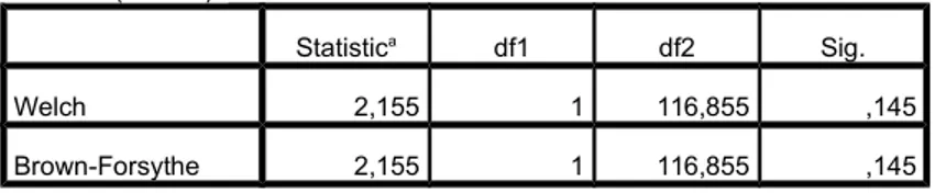
Since the assumption of homogeneity of betweengroup variance is rejected for Skills, Luck and Mood, we decided to use independent oneway ANOVA to explore the univariate outcome, by additionally employ Brown–Forsythe F and Welch’s F test.

Levene's Test of Equality of Error Variancesa

F df1 df2 Sig.

A. Skills 1,314 7 111 ,250

B. Luck ,642 7 111 ,721

C. Mood 1,643 7 111 ,131

D. Efforts 1,942 7 111 ,070

E. Easy game 3,170 7 111 ,004

Tests the null hypothesis that the error variance of the dependent variable is equal across groups.

(27)

Table 20: Leven's Test for equality of variances

Univariate ANOVA:

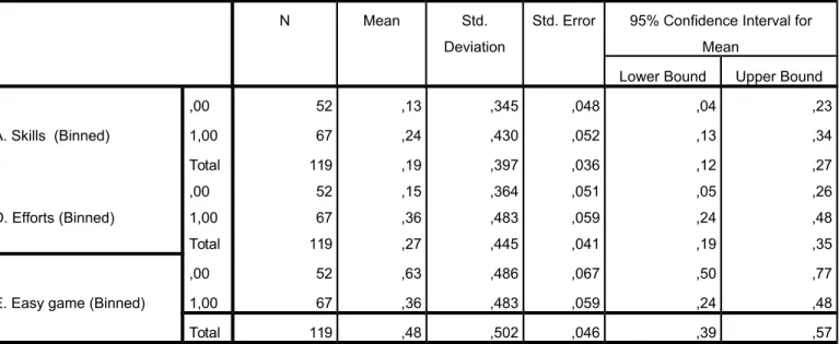
We performed separate analyses of variance (ANOVA) to check further relationships between independent and dependent variables. For the design was Skills x RichVsPoor, the analyses did not show significant difference for the dependent variable Skills per Rich and Poor groups. Welch: F (1, 166..885) = 2.155, p = 0.145. This is due to the fact that the violation of homogeneity hypotheses poses threat to the validity of the previous result. (See appendix VII). Regarding the analyses of ANOVA Effort x RichVsPoor, the results confirm that there is still a highly significant difference in Effort per Rich and Poor participants groups Welch: F(1, 166.920) = 6.919, p = 0.010.

ANOVA means

N Mean Std.

Deviation

Std. Error 95% Confidence Interval for Mean

A. Skills (Binned)

,00 52 ,13 ,345 ,048 ,04 ,23

1,00 67 ,24 ,430 ,052 ,13 ,34

Total 119 ,19 ,397 ,036 ,12 ,27

D. Efforts (Binned)

,00 52 ,15 ,364 ,051 ,05 ,26

1,00 67 ,36 ,483 ,059 ,24 ,48

Total 119 ,27 ,445 ,041 ,19 ,35

E. Easy game (Binned)

,00 52 ,63 ,486 ,067 ,50 ,77

1,00 67 ,36 ,483 ,059 ,24 ,48

Total 119 ,48 ,502 ,046 ,39 ,57

Table 21: RichVSPoor

(28)

N Mean Std. Deviation Std. Error 95% Confidence Interval for Mean

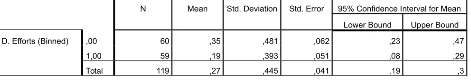
D. Efforts (Binned) ,00 60 ,35 ,481 ,062 ,23 ,47

1,00 59 ,19 ,393 ,051 ,08 ,29

Total 119 ,27 ,445 ,041 ,19 ,3

Table 26: BJW_lowhigh

The table above shows the ANOVA means for Effort and the independent variable BJW_lowghigh. From Table 21 we notice that people in the low BJW group assign a higher score to Efforts respect to people in the high BJW group, even if the 95% confidence intervals overlap a little bit.

Continuing, Easy game x RichVsPoor confirm that there is a significant difference in Easy game per Rich and Poor participants groups Welch: F(1, 102.961) = 3.859, p = 0.052. (see Appendix VIII, table 15 and 16). When considering Effort x BJW Table 17 and Table 18 confirm that there is still a highly significant difference in Effort per BJW (low and high) groups. Welch: F(1, 113.201) = 4.134, p = 0.044.

Donated Money

(29)

BJW_lowhigh * Donated Money (Binned) Crosstabulation

Donated Money (Binned) Total

No donated money Less than 32.7 between 32.8 and 66.4 more than 66.5 BJW_lowhigh ,00

Count 13 15 21 10 59

% within BJW_lowhigh 22,0% 25,4% 35,6% 16,9% 100,0%

% within Donated Money (Binned)

37,1% 50,0% 61,8% 52,6% 50,0%

% of Total 11,0% 12,7% 17,8% 8,5% 50,0%

1,00

Count 22 15 13 9 59

62,9% 50,0% 38,2% 47,4% 50,0%

% of Total 18,6% 12,7% 11,0% 7,6% 50,0%

Total

Count 35 30 34 19 118

100,0% 100,0% 100,0% 100,0% 100,0%

% of Total 29,7% 25,4% 28,8% 16,1% 100,0%

Table 27: Crosstabulation Donated money and BJW

Table 27 allows us to understand that low believers tend to donate an amount of money be tween 32.8 and 66.4, while high believers tend to do not donate any money.

Symmetric Measures

Value Approx. Sig.

Nominal by Nominal Phi ,190 ,236 Cramer's V ,190 ,236

N of Valid Cases 118

Table 28: Symmetric measure

Chi-Square Tests

Value df Asymp. Sig. (2-sided)

(30)

Linear-by-Linear Association 2,683 1 ,101

N of Valid Cases 118

a. 0 cells (0,0%) have expected count less than 5. The minimum ex-pected count is 9,50.

Table 29: Chisquare test

Table 27 shows us that there is no statistically significant association between Donated Money and BJW, \chi^2 = 4.249, p = 0.236

(31)

As can we notice from Figure 3 and the bar chart even if it seems that low believers prefer to donate a particular amount of money while high believers prefer to do not allocate any money, since we have no statistically significant association between these 2 variables, we expect that by repeating the experiment the results may vary a lot.

4. Discussion

In the present study observer's reactions (attributions of success/failure/donated money) of winning and losing in a rigged Monopoly scenario were examined as they are affected by observer's BJW and advantage and disadvantage in players starting position.

We expected that high believers in a just world will be convinced that the actor's success is due to Skills and Effort, more than other attributes like Luck, Easy Game or Mood. Specifically, we hypothesized that this will happen in the rich (advantage condition), where the actor was in advantageous position (started with 100€). In addition, observers in both conditions were

turned into actors and asked to donate the won money to a charity institution of their choice: we predicted that high believers in a just world would allocate less fairly. In regards to the low believers in the rich condition, we assumed that subjects will not believe the player deserved to win and therefore would allocate success to the factors of Mood, Luck and Easy game and less to Skills and Effort.

Rich people believed more in effort; High on BJW people believed more in effort

(32)

that observer's attribution to Effort, to explain success or failure was high in comparison to the rest of the attributions. Furthermore, the strong positive correlation between the internal traits  Effort and Skill tends to show that observers who agreed with the fact that the game is won/lost by efforts also agreed with the fact that the game was won thanks to Skills. Consistent with the present study Weiner (1994), also found that although there may be an almost infinite number of determinants of academic success and failure, perceived causes

among students are mostly attributed to ability and effort and commonly to task difficulty and luck. (Weiner,1994).

In our examined sample, observers that scored high on belief in a just world attributed actor's behavior to the internal/unstable cause of Effort. Effort is more variable and can change from situation to situation. As expected our subjects tended to attribute Effort to success in an obviously unfair Monopoly game. In fact, results are congruent with the early study made by Lerner in 1965, where he explained to observers that the fairest way of selecting one worker for payment is by chance and that the workers had to drawn numbers from a hat to decide whether they belonged to the paid or the unpaid group. Next, the observers listened how the workers solved anagrams, and then they rated the performance and personal characteristics of both workers. Consistent with a belief in a just world, observers rated the performance of the paid worker as superior to that of the unpaid worker. In the present study a new element was introduced. Observers did not rate actors performance, but they “judged” their attribution of success and failure, attributing it to different causes. In Lerner's study, subjects imposed justice on the situation by persuading themselves that the paid worker deserved to be rewarded — “he must have contributed more than the unpaid worker”. Similar happened in our study: observers tend to believe that thanks to their Effort, actors in the rich, but unfair condition, won the game.

(33)

justifying beliefs. It seems that in his research the perceptions of actor's own behavior were influenced by situational outcomes, while in our study observers perceived behavioral outcomes – their Effort. In our sample, we provide some evidence for Effort attribution, when observers score high on BJW and starting unfairly the game (rich condition). Further, Jones and Nisbett's (1971) gave an answer in their analysis of the perception of the causes of behavior. They contend that observers watching an actor focused primarily on the actor's behavior, while the actor's attention focuses on his environment. An observer attending closely to a recipient's behavior, for instance, may miss situational cues involving the arbitrary nature

of a chance outcome and, instead, "see" an explanation for the outcome within the recipient. As predicted, the low BJW group tend to assign a higher equal score to all the dependent variables except from Easy Game with respect to the high BJW group. Participants did not attribute Mood, Skill, Luck differently in the experimental conditions (starting rich or poor:, high or low in BJW) to explain success or failure. The effects of the interaction between these independent variables on attribution and donation were not significant and were deleted in order not to lose analysis power. The negative correlation between Fairness and Skill implicates that probably participants who evaluated the game as being won/lost thanks to high

Skills evaluated the game to be less fair. One reasonable and probable answer would be that

subjects understood the unfair rules with which the game started and that a better scenario set up must be examined.

Rich/Poor did not differentiate between Skills. Observers in both conditions attributed success as well as failure in even amounts to Skills or the lack of skill. It might be that participants evaluated the game as more unfair the more they thought that Skills mostly out of control of the actor – was so important to win/loose the game.

(34)

focused people opt to organize more donating initiatives and are aware of greater number of charity organizations and causes. (e.g., Erez & Earley, 1987; Hofstede 2001; Wagner,1995). Moreover, from the correlation analyses we can see that people who tend to believe it was an Easy game showed tendency to donate more money in general. This could lead us to believe that individuals who do not perceive high Effort are more prone to donate in comparison to people who really believed they deserved the money because of their high effort. Consistent with Piff, people who believe they perform better and involve more effort develop entitlement believing they deserve it and have the right to it. They are more likely to believe that greed and selfinterest is a moral and good thing, therefore less prone to donate.

Finally, there are many errors that can occur while making attributions of success or failure. And many aspects of this study could have been done better. Our participants are not excluded from the possibility of being biased by actorobserver effect for instance. Past achievements also contribute to the mind set of deservningness and achievement regardless the given culture of the situation, so its possible that subjects got biased. The work of McClelland, Clark, Lowell and Atkinson (1953) working primarily with adults, suggests that people who are high on the need for achievement, have some belief in their own ability or skill to determine the outcome of their efforts.

A number of limitations should be considered when interpreting the results. Most notably, the nature of the sample used in such an investigation may limit the extent to which these findings can be generalized. The application of the study was only applied to a certain self chosen group. The study among mostly students must be replicated among individuals sampled from a wider population group. We also assume that if we were to include a mood scale in order to determine the positive or negative mood, our participants could have revealed different results, as substantial amount of literature states that mood influences attributions. (see Bower, 1981). Likewise, the scale of selfesteem would have probably yield more detailed outcome to complete the picture of allocation, attribution and justifications. Lastly, post examination of feelings about money allocation should be included too to check people's satisfaction when allocating money to their favorable charity cause.

(35)

to give affirmative responses; negative responses; extreme responses; uncertain responses or socially desirable responses. It has been found, for example, that blacks are more likely than whites to give extreme responses in Likerttype questionnaires (Bachman & O'Malley, 1984). Furthermore, although all the subjects of the study had a good command of English, some do not have English as their native language, and certain expressions may have different connotations for different language groups. Especially, when filling in the BJW scale where American expressions were predominant. It is important to note, the subjects of the study were not remunerated or given credits, and it is therefore possible that the most unmotivated members of the population may have been elected. Moreover, the sample size was too small, future studies should include bigger samples. Given the fact of marginal significance, we reckon that if all 332 participants filled in the questionnaire correctly, we would have obtained

more significant results.

The present paper is the first step to study a newly developed scenario of rigged Monopoly game and how observers deal with inequality during allocation processes. We are aware that a deeper examination of this question requires additional avenues of research. A possible approach to our experiment and strongly recommended one is to execute it with a bigger randomly selected sample as well as executing it in lab settings, rather than online.

(36)

R E F E R E N C E S:

•

Bachman, J.G., & O'Malley, P.M (1984). Blackwhite differences in selfesteem. Are they different in response style. American Journal of Sociaology, 90, 624639

•

Bower, G. H. (1981). Mood and memory. American Psychologist, 36(2), 129148

 Cohen, J. (1988) Statistical power analysis for the behavioral sciences (2nd ed.).

Hillsdale, NJ: Erlbaum, 98

 Cortina, Jose M. (1993) "What is coefficient alpha? An examination of theory and appli cations." Journal of applied psychology Vol. 78. N: 1, 98.

 Cozzarelli, C., Wilkinson , A., Tagler, J. (2001) Attitudes Toward the Poor and Attribu tions for Poverty , Journal of Social Issues, Vol. 57, No. 2, pp. 207–227

 Cropanzano, R., Mitchell, M. S. (2005) Social Exchange Theory: An Interdisciplinary Re view,Journal of Management, Vol. 31 No. 6, December 2005 874900

 Crandall, C. S. (1994). Prejudice against fat people: Ideology and selfinterest. Journal of Personality and Social Psychology, 66, 882894

 Erez, M. & Earley, P.C. (1987) Comparative analysis of goalsetting strategies across cultures. Journal of Applied Psychology, Vol. 72: 658665

(37)

 Foa, U.G (1971) Interpersonal and Economic Resources, Science Vol. 71, 346349

 Foa. Ugriel G. and Edna Foa (1974). Societal Structures of the Mind, Springfield, IL:

Charles C Thomas. 452

 Greenberg, J, (1979). Protestant ethic endorsement ad the fairness of equity inputs. Journal of Research in Personality, Vol. 13, 819

 Hafer, C.L., Belgue, L. (2005) Experimental Research on JustWorld Theory: Problems, Developments, Psychological Bulletin Vol. 131, No. 1, 128 –167

 Hofstede, G. (2001) Culture's Consequences: Comparing Values, Behaviors, Institutions and Organizations Across Nations. 2nd Edition, Thousand Oaks CA: Sage Publications

 Heider, F. (1958). The psychology of interpersonal relations. New York: Wiley, 1958. 322.

 Jones, E. & Nisbett, R. (1971) The actor and the observer: Divergent perceptions of the causes of behavior . New York: General Learning Press, 7994

 Jost & Pelham & Carvallo (2002) Nonconscious forms of system justification: Implicit and behavioral preferences for higher status groups. Journal of Experimental Social

Psychology , Vol 38, 586602

 Kahneman, D and Tversky, A. (1991) Loss aversion in a rickless choice: A reference dependent model. The quarterly Journal of Economics, Vol. 106, N: 4, 10391061

 Katz, I., Hass, R. (1988) Racial ambivalence and American value conflict: Correlational and priming studies of dual cognitive structures. Journal of Personality and Social

(38)

 Kelley, H., (1967) Attribution theory in social psychology. In D. Levine (Ed.), Nebraska

Symposium on Motivation Vol. 15, 129–238. Lincoln: University of Nebraska Press

 Kelley, H., (1973) The Processes of Causal Attribution University of California, Los

Angeles, American Psychologists 107128

 Kline, P. (1999). The handbook of psychological testing (2nd ed.). London and New York: Routledge

 Kluegel, R. Eliot R. (1986) Beliefs about Inequality: Americans' View on What is and What Ought to be. Rutgers The State University, New Jersey, 332

 Lerner, M. J. (1980). The belief in a just world. A fundamental delusion New York: Plenum Press

 Lerner, M. J. (1965). Evaluation of performance as a function of performer's reward and attractiveness. Journal of Personality and Social Psychology, 1(4), 355360

 Lerner, M. J. (1970) The desire for justice and reactions to victims. In J. Macaulay and S. L. Berkowitz (Eds.), Altruism and helping behavior. New York: Academic Press

 Lerner, M. J., & Simmons, C. H. (1966) The observer’s reaction to the “innocent victim”: Compassion or rejection? Journal of Personality and Social Psychology, Vol. 4, 203210.

 Lerner, M. J., & Matthews, (1967) G. Reactions to suffering of others under conditions of indirect responsibility. Journal of Personality and Social Psychology, Vol. 5, 319325.

(39)

scale. Personality and Individual Differences, Vol. 12, 11711178

 Major, B. Cheryl, R., Shannon, K.,McCoy, K, (2003) It’s Not My Fault: When and Why Attributions to Prejudice Protect SelfEsteem, Personality and Social Psychology Bulletin

Vol. 29 No. 6, 77278

 McClelland, D. C., Atkinson, J. W., Clark, R. A., & Lowell, E. L. (1953). Century psychology series. The achievement motive. East Norwalk, CT, US: AppletonCentury

Crofts.

 McCoy & Major (2006) Priming meritocracy and the psychological justification of inequality, Journal of Experimental and Social Psychology,Vol. 43, 341351

 Piff, Stancato, Côté, MendozaDenton, Keltner (2012) Social class predicts increased unethical behavior, PNAS Vol. 109, N: 11, ,4086–4091

 Piff, P. (2014) in press “Does Money make you mean”

http://tedsummaries.com/2014/09/05/paul-piff-does-money-make-you-mean/ retrieved from ted.com on September 5th_, 2014

 Rotter, J . B. (1966). Generalized expectancies for internal versus external control of reinforcement. Psychological Monographs: General and Applied , Vol. 80 , N 1 – 609

 Rubin, Z., & Peplau, L. A. (1975). Who believes in a just world? Journal of Social

Issues,Vol. 31(3), 65–89

 Vermunt, (2014) The Good the bad and the just: How modern man shape their world, London: Ashgate.

(40)

cooperation in group. Academy of Management Journal Vol.38, 152172

 Weiner B, Nierenberg R. & Goldstein, M (1974) Social learning (locus of control) versus attributional (causal stability) interpretations of expectancy of success, Journal of Personality Vol 44,1, 52–68

(41)

(42)

APPENDICES I

BJW Scale:

1. Just World Scale by Z. Rubin & L. A. Peplau Just world scale (1975)

Instructions:

Indicate your degree of agreement or disagreement with each of the following statements in the blank space next to each item. Respond to every statement by using the following code.2

5 = strongly agree 4 = moderately agree 3 = slightly agree 2 = slightly disagree 1 = moderately disagree 0 = strongly disagree

1 . I’ve found that a person rarely deserves the reputation he has. 2. Basically, the world is a just place.

3. People who get “breaks” have usually earned their good fortune.

4. Careful drivers are just as likely to get hurt in traffic accidents as careless ones. 5. It is a common occurrence for a guilty person to get off free American courts. 6. Students almost always deserve the grades they receive in school.

7 Men who keep in shape have little chance of suffering a heart attack. 8. The political candidate who sticks up for his principles rarely gets elected. 9. It is rare for an innocent man to be wrongly sent to jail.

10. In professional sports. many fouls and infractions never get called by the referee. 11. By and large, people deserve what they get

12. When parents punish their children. it is almost always for good reasons. 13. Good deeds often go unnoticed and unrewarded.

14.Although evil men may hold political power for a while in the course of history, good wins out 15. In almost any business or profession. people who do their job well rise to the top.

16. American parents tend to overlook the things most to be admired m their children. 17. It is often impossible for a person to receive a fair trial in the USÆ

18. People who meet with misfortune have often brought it on themselves. 19. Crime doesn’t pay.

20. Many people suffer through absolutely no fault of their own.

(43)

APENDIX II

Table 1:Reliability Statistics considering 20 items

Reliability Statistics

Cronbach's Alpha Cronbach's Alpha Based on Standard-ized Items

N of Items

,664 ,650 20

(44)

(45)

(46)