BAS: A Perceptual Shape Descriptor Based on the Beam Angle Statistics

BAS: A Perceptual Shape Descriptor Based on the Beam Angle Statistics Nafiz Arica and Fatos T. Yarman Vural

Computer Engineering Department,

Middle East Technical University, Ankara / Turkey {nafiz,vural}@ceng.metu.edu.tr

Abstract

The proposed shape descriptor is based on the beams originated from a boundary point, which are defined as lines connecting that point with the rest of the points on the boundary. At each point, the angle between a pair of beams is calculated to extract the topological structure of the boundary. Then, a shape descriptor is defined by using the third order statistics of all the beam angles in a set of neighborhood systems. It is shown that Beam Angle Statistics (BAS) is invariant to translation, rotation, scale and is insensitive to distortions. Experiments are done on the dataset of MPEG 7 Core Experiments Shape-1. It is observed that BAS outperforms the MPEG 7 shape descriptors.

Keywords: Shape Representation, Shape Description, Beam Angle Statistics (BAS), Optimal Correspondence

1. Introduction

The advances in MPEG-7 activities for content-based description of images come to a point to represent the shape information in a standard format, which allows searching and browsing images in a database with respect to the shape information. The goal of the shape descriptors is to uniquely characterize the object shape. The shape descriptor is expected to be affine-invariant and insensitive to noise. It should contain sufficient information to resolve distinct images and compact enough to ignore the redundancies in the shapes. Additionally, the descriptors should give results consistent to human visual system. Therefore, it is desirable to find a shape descriptor, which represents the perceptual shape information in a simple function.

The shape description methods can be divided into three main categories, (Latecki 2000); contour based (Mokhtarian 1997), (Latecki 2000.1), (Chuang 1996), image based (Khotanzan 1990) and skeleton based descriptors (Lin 1996). In the Core Experiment CE-Shape-1 for the MPEG-7 standard, the performance of above referenced shape descriptors are evaluated. Among them, the descriptors proposed in (Mokhtarian 1997) and (Latecki 2000.1) outperform the others in most of the experiments. In (Mokhtarian 1997), the scale space approach is applied to shape boundary. The simplified contours are obtained by the scale-space curve evolution, based on contour smoothing with a Gauss function. The scale space image of the curvature function is then used as hierarchical shape descriptor. In (Latecki 2000.1), the scale of shapes are reduced by a process of curve evolution and represented in tangent space. To compute the similarity measure, the best possible correspondence of visual parts is established. However, none of the available techniques extract the shape information independent of context and has limited performance under noise. Therefore, in order to fully utilize the shape information with its full power, more research is required.

The motivation of this paper is to find a representation of the two-dimensional shape information without a predefined context-dependent scale. This requires a mapping, which transforms the 2-D

shape information into 1-D function, which is consistent with the human visual system. In other words, this function should represent all the convexities and concavities of the shape with minimal distortion.

The proposed descriptor is based on the beams, which are the lines connecting the reference point with the rest of the points on the boundary. The characteristics of each boundary point can be extracted by using the beams at a set of neighborhood systems. The angle between each pair of beams is taken as the random variable at each point on the boundary. Then, the moment theorem provides all the statistical information, which is used to obtain the desired function where each valley and hill corresponds to a concave and convex visual part of the object shape respectively. After the representation of 2-D shape boundary as a 1-D function, the optimal correspondence algorithm is employed for similarity measurement.

The main contribution of this study is to eliminate the use of any heuristic rule or empirical threshold value in representation of shape boundaries in a predefined scale. The proposed method also gives globally discriminative features to each boundary point by using all other boundary points. Another advantage of this representation is its simplicity yet consistency with human perception through preserving the concave and convex parts of the shapes. It provides and compact representation of shapes, which is insensitive to noise and affine transform and is invariant to size, orientation and position of the object.

After giving the previous relevant study in section 2, section 3 introduces the proposed shape descriptor. The similarity measurement is described briefly in section 4. The similarity tests, performed on a data set of MPEG Core Experiments, is explained in section 5. Finally, section 6 concludes the paper and directs the future studies.

2. K-Curvature Function

The significance of curvature information at object boundaries has been an inspiration of many studies related to shape analysis (Loncaric 1998). A variety of algorithms use high curvature points as corners and approximate the shape by a polygon (Latecki 2000.1). Another curve approximation scheme is based on splines, which posses the beneficial property of minimizing curvature (Cohen 1995). In some studies, the shape is decomposed into parts at points of high negative curvature (Siddigi 1996). Scale space techniques are applied to shape boundary by filtering with Gaussian kernels of increasing width to obtain a multi-scale representation of curvature (Mokhtarian 1986). The curvature function is directly used to represent the shape boundary in (Urdiales 2002).

The curvature function basically describes how much a curve bends at each point of shape boundary and is defined as the rate of change of the curve slope θ (s) with respect to its length s. The slope angle of a curve, Γ(s)=(x(s),y(s)), is given by

( )

dx dy s = − θ

( )

( )

( ) ( ) ( ) ( )

( )

( )

(

)

The above calculation of curvature requires second derivatives, which is not practical for discrete curves. For this purpose, curvature based shape description methods use some heuristics. In (Mokhtarian 1986), the shape boundary is filtered by Gaussian function and the curvature is calculated directly along the smoothed curve definition. Another study uses the edge gradient at each point by the arctangent of its Sobel difference, in a 3x3 neighborhood (Liu 1990).

The curvature function can be computed as the derivative of the contour’s slope function. In order to prevent noise in the slope function caused by fluctuations on the boundary, some smoothing is introduced into the slope evaluation. This can be performed by K-slope method. K-slope at a boundary point is defined as the slope of a line connecting that point with its Kth right neighbor. Then, the K-curvature at a boundary point is defined as the difference between the K-slope at that pixel and the K-slope of its Kth left neighbor.

The K-curvature function may be exploited to form an appropriate shape descriptor, if one could identify an optimal value for the parameter K. Because; for a fixed K, the plot of K-curvature function represents a one-dimensional function, which extracts the concavities and convexities of the shape at a predefined scale settled by K.

At this point, we need a rigorous technique to identify the scale parameter K, which discriminates a wide range of shapes in large image databases. In (Agam 1997), the curvature function is obtained by using a fixed K value and then it is filtered in order to stress the main features. Another study (Urdiales 2002) uses an adaptive K value by changing it according to the distance between relevant points. It is also possible to estimate an “optimum” value for K using the popular training methods. However, choosing a single K value cannot capture the exact curvature information for all varieties of shapes in the database. In addition, the heuristics used in estimation of K may not be valid for some shapes.

3. BAS: A Shape Descriptor with Beam Angles Statistics

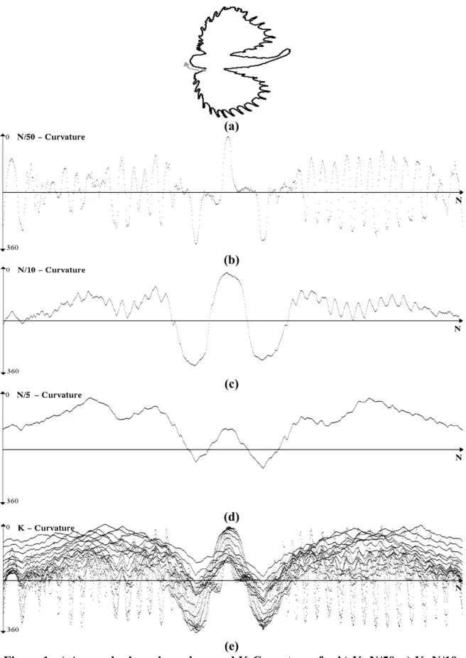
Let us start by investigating the effect of the parameter K on the resolution of the K-curvature representation. Figure 1 b, c and d indicate the plot of K-curvature function for a sample shape with various K values. Note that the plots for small K capture fine details. By increasing K, it is possible to plot fine to curse representation of a closed boundary as a one-dimensional function. Examining these figures shows that each peak and valley of the curvature function plot corresponds to a convexity, and a concavity of the shape. For this particular example, the shape information is preserved in the peaks corresponding to the head, tail and fins. The remaining peaks and valleys of the curvature plot are rather redundant details, that result from the noise in the shape, leading mismatches in the image database. Therefore, one needs to select an appropriate K to avoid this redundant information.

(a) (b) (c) (d) (e)

Figure 1. a) A sample shape boundary and K-Curvatures for b) K=N/50, c) K=N/10, d) K=N/5 and e) the superposition of K = N/50…N/5 from top to bottom respectively.

Visual inspection of Figure 1, indicates that in order to capture the perceptually meaningful concavities and convexities, K= N/10 may be an appropriate choice to represent the silhouette of the fish. As we decrease the value of K to N/50, we obtain too many spurious peaks, whereas increasing the K value to N/5 yields a representation, which lacks the peaks and valleys corresponding to important perceptual information. Therefore, selection of K defines the amount of smoothing of the shape and highly depends on the context of the image. If K smoothes the ripples corresponding to some context information, this will result in important information loss. On the other hand, if the ripples correspond to noise, keeping them will increase the number of convexities and concavities, which may carry superfluous shape information. As a result, the problem of selecting a generic K, which resolves the necessary and sufficient information for all the images, has practically no solution, due to the diversity of the shape context in large databases.

The above discussion leads us to somehow find a representation, which employs the information in K-curvature function for all values of K. This representation should be compact enough to yield a shape descriptor. Superposition of the plots of K-curvature function for all K, yields impractically large data with no formal way of representation, as indicated in figure 1.e.

In this study, we attack this problem by modeling the shape as the outcomes of a stochastic process, which is generated by the same source at different scales. In this model, Figure 1.e shows the possible outcomes of the shape curvature plot, which generates the fish shape. At a given boundary point p(i), the value of K-curvature function is assumed to be a function of a random variable K and may take one of the values indicated in the figure, depending on the values of K. Therefore, K-curvature function can be considered as the output of a stochastic process. In the following formalism, we introduce the beam angle which is closely related to the curvature slope.

Mathematically speaking, let the shape boundary B = { p(1),...,p(N)} is represented by a connected sequence of points,

(

)

)

(i xi y i i N

p = =

where N is the number of boundary points and p(i) = p(i+N). For each point p(i), the beams of p(i) is defined as the set of vectors

( )

(

)

{

}

L = + −

where Vi+j and Vi-j are the forward and backward vectors connecting p(i) with the points, p(i+j) and p(i-j) in the boundary, for j=1,…N/2 .Figure 2.a indicates the beams of a point p(i).

Also, the Kth _{order neighborhood system is defined as}

p(i±K)∈η_K (p(i)) ∀p(i), i=1...N, K =1...N/2 (5)

Note that, for each neighborhood system K, there is only one pair of beams, connecting p(i) to p(i+K) and p(i-K). Figure 2.b indicates the pixels in different neighborhood systems.

(a) (b) Figure 2. a)The beams of point p(i), b) the neighborhood systems. The slope of each beam , Vi+k is then calculated as,

) 6 ( , tan 1 l k x y l i l i Vi l ∆ =± ∆ = + + − + θ

For the point p(i), the beam angle between the forward and backward beam vectors in the kth _order

neighborhood system, is then computed as (see figure 3).

(

)

)

( _{Vi k Vi k}

K i

C = θ ₋ −θ ₊

Note that, beam angle at a neighborhood system K is nothing but the K-curvature function. (which takes values between 0 and 2π).

Figure 3. The 5-Curvature and the beam angle at the neighborhood system 5 for the boundary point p(i) .

Now, for each boundary point p(i) of the curve Γ, the beam angle CK(i) in the neighborhood

system ηK can be taken as a random variable with the probability density function PK(CK(i)) and

different scales. Therefore, Beam Angle Statistics BAS, may provide a compact representation for a shape descriptor. For this purpose, mth moment of the random variable CK(i) is defined as follows:

[ ]

∑

In the above formula E indicates the expected value operator and PK(CK(i)) is the probability density

function of CK(i). Note that the maximum value of K is N/2, where N represents the total number of

boundary points. Note also that, the value of CK(i) approaches to 0 as K approaches to N/2. During

the implementations, PK(CK(i)) is approximated by the histogram of CK(i) at each point p(i).

The moments describe the statistical behavior of the beam angle at the boundary point p(i). Each boundary point is then represented by a vector whose components are the moments of the beam angles:

[

]

)

(i = ΕC1 i ΕC2 i

Γ

The shape boundary is finally represented by plotting the moments of CK(i)’s for all the boundary

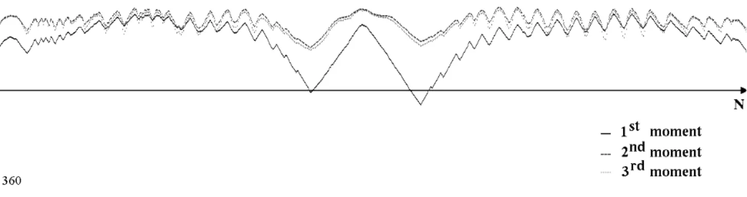
points. In the proposed representation, the first moment preserves the most significant information of the object. Figure 4, indicates the first three moments of boundary points for the sample shape of figure 1.a. For this particular example, it should be noted that the first moment suffice to represent the convexities and concavities of the shape. The second moment increases the discriminative power of the representation. The third moment on the other hand, does not bring any additional significant information to the representation. The order of the statistics naturally depends on the characteristics of the probability density function, PK(CK(i)). Central limit theorem provides us a strong theoretical basis to assume Gaussian distribution for each point p(i) for large N. This implies that second order statistics is sufficient for representing most shapes provided that we have enough samples on shape boundary.

Figure 4) Third order statistics of Beam Angle for the shape in figure 1.a.

The representation, explained above, allows us to compare any shapes as long as they are specified by simple closed curves. It is invariant to size, orientation and position of the object and is insensitive to distortions and shear transform.

4. Similarity Measurement

The similarity between the features, extracted from the BAS moment functions of shape boundaries, is measured by Optimal Correspondent Subsequence (OCS) algorithm (Wang 1990). The OCS method was developed for infinite alphabet string matching problem. The objective in similarity measurement is to minimize the distance between two vectors by allowing deformations. This is achieved by first solving the correspondence problem between items in feature vectors and then computing the distance as a sum of matching errors between corresponding items.

The similarity measurement of the proposed shape descriptor considers each feature vector extracted from BAS function as an integer number string. For this purpose, equal length feature vectors are generated by sampling the BAS functions. The distance between two number strings is then calculated by the OCS algorithm. In minimization of total distance between corresponding items, the dynamic programming technique is employed by building a minimum distance table which accumulates the information of correspondence.

Mathematically speaking, let Γ and Π be two feature vectors with N and M points respectively. A matching is defined by a function, t(i), so that the point Γ(i) is mapped to the point Π(t(i)). Then, the minimization of total matching cost can be formalized as

) 10 ( )) ( ( ), ( ( ) , (

min

∑

where dist(Γ(i), Π(t(i)) represents the distance between individual points Γ(i) and Π(t(i)). It is defined by ( (), ( )) ( (), ( )) (11) 2

∑

where l represents the moment order. The distance function given above is not a Euclidean distance but the square of the Euclidean distance. Euclidean distance is not used in order to save computations. Losing the linearity of the Euclidean distance is acceptable, considering the serious impact in the reduction of computation time.

The minimization problem in (10) can be solved efficiently and optimally by using the below recurrence relation (Wang 1990),

[

] [

] [

]

{

}

In the above formula, D(i,j) is the cumulative distance to point Γ(i)and Π(j) and t is a constant. Starting with D(0,0) = 0, the cumulative distance recurrence relation is used to obtain the optimal correspondence of points. The three terms of the above relation can be explained as follows; the first term matches Γ(i) with Π(j), the second term leaves the Γ(i) unmatched and the third term skips Π(j) without matching any item from Γ.

By iterating over i and j, D(N,M) which equals the total cost of matching COST(Γ, Π) , is computed. The algorithm for the correspondence problem in the similarity measurement is given below:

OPTIMAL CORRESPONDENCE ALGORITHM

[

]

[

]

[

] [

] [

]

{

(

)

In the above algorithm , t is taken as the distance between the individual points instead of a constant. Note also that the time complexity of this algorithm is quadratic. This method is more efficient than relaxation (Davis 1979) and elastic matching (DelBimbo 1997) for one-dimensional problems.

5. Experiments

The performance of BAS descriptor is evaluated by comparing it with the other studies in the literature using the data set of MPEG 7 Core Experiments Shape-1. It is, then, tested to investigate the stability under noise, affine transformation and smoothing by polygonal approximation.

The boundaries of objects are represented by the BAS descriptor using the third order statistics. Then, the optimal correspondence algorithm is employed for similarity measurement.

The goal of the MPEG 7 CE-Shape-1 is to evaluate the performance of 2D shape descriptors under the below conditions (Latecki 2000),

• change of a view point with respect to the objects,

• non-rigid object motion

• noise.

The shapes are restricted to the simple pre-segmented shapes defined by their outer closed contour. The main requirement is that the shape descriptors should be robust to small non-rigid deformations and scale and rotation invariant. The core experiment is divided into three parts with the following objectives:

PART A: Robustness to Scaling and Rotation

A-1 Robustness to Scaling: The database contains 420 shapes; 70 basic shapes and 5 derived shapes from each basic shape by scaling digital images with factors 2, 0.3, 0.25, 0.2 and 0.1. Each of the 420 images was used as a query image. A number of correct matches was computed in the top 6 retrieved images. Thus the best possible result is 2520 matches.

A-2 Robustness to Rotation: The database contains 420 shapes; the 70 basic shapes are the same as in part A-1 and 5 derived shapes from each basic shape by rotation with angles 9, 36, 45, 90 and 150 degrees. Each of 420 images was used as a query image. A number of correct matches was computed in the top 6 retrieved images. Thus the best result is 2520 matches.

PART B: Similarity-based Retrieval

This is the main part of the Core Experiment CE-Shape-1. The total number of images in the database is 1400; 70 classes of various shapes, each class with 20 images. Each image was used as query and the number of similar images, which belong to the same class was counted in the top 40 matches. Since the maximum number of correct matches for a single query image is 20, the total number of correct matches is 28000.

PART C: Motion and Non-Rigid Deformations

Part C add a single retrieval experiment to part B. The database for part C is composed of 200 frames of a short video clip with a bream fish swimming plus a database of marine animals with 1100 shapes. Fish bream-000 used as query and the number of bream shapes in the top 200 shapes was counted. Thus, the maximum number of possible matches was 200.

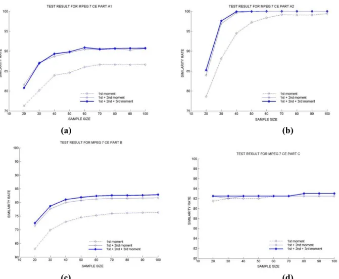
BAS moment functions are sampled with equal distance to extract the feature vector. Various sample sizes between 20 and 100 are tested to see the stability of the proposed descriptor to the sampling rate. Figure 5 a, b, c and d indicate the similarity rate of the BAS descriptor with respect to the size of the feature vector for MPEG 7 Core Experiment Shape 1 part A1, A2, B and C. The similarity rate in each experiment is calculated by taking the ratio of correct matches in the maximum number of possible matches. As it is seen from the figure while the similarity rate remains almost unchanged after size 60 for Part A1 and C, it is constant after 40 samples in Part A2 and same for all values for Part C. Note that the sampling process is not applied on the original shape, but just on the moment functions. Therefore, the sampling rate does not directly affect the scale if it is above the Nyquist rate.

The shape descriptors to be evaluated by the above test data, can be divided into three main categories:

• Contour-based descriptors; P320 which uses the curvature scale-space (Mokhtarian 1997), P567 which uses the wavelet representation (Chuang 1996), P298 which uses tangent space and the best possible correspondence of visual parts (Latecki 2000.1) and recent study called shape context (Belongie 2002).

• Image-based descriptors; P687, which uses the Zernike moments (Khotanzan 1990), P517 which uses the multiplayer eigenvectors.

(a) (b)

(c) (d)

Figure 5: Similarity rates in MPEG CE Shape-1 data, as a function of the sample size, a) Part A1, b) Part A2, c) Part B, d) Part C.

Table 1 indicates the comparison of the proposed descriptor with the reported results of the recent studies. Note that the BAS descriptor has a better performance in most of the experiments, especially in Part B, which is the most difficult part of the MPEG CE Shape-1. Note that Part B, contains classes with significantly different shapes and distinct classes with similar shapes. Therefore, one does not expect to reach a retrieval rate of 100% (see figure 6.).

TABLE 1. COMPARISON OF BAS WITH THE RECENT STUDIES Data Set Shape Context Tangent Space Curvature Scale Space Zernika Moments

Wavelet DAG BAS With 40 Samples BAS with 60 samples PartA1 - 88.65 89.76 92.54 88.04 85 89.32 90.87 PartA2 - 100 99.37 99.60 97.46 85 99.82 100 PartB 76.51 76.45 75.44 70.22 67.76 60 81.04 82.37 PartC - 92 96 94.5 93 83 93 93.5

(a)

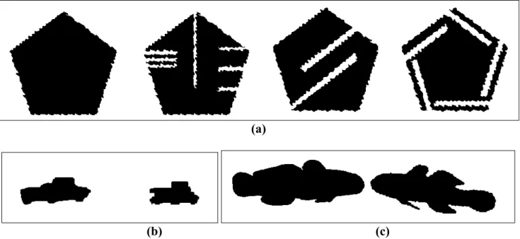
(b) (c) Figure 6: Sample shapes from MPEG CE Shape-1 Part B. a) Shapes from the same class

device6, Shapes from the different classes b) car and truck classes, c) fish and imfish classes. Average performance with the average over three parts (Total Score 1) and the average over the number of queries (Total Score 2) is given in Table 2. In terms of both of the performance criteria, BAS outperforms all the studies.

TABLE 2. COMPARISON OF AVERAGE PERFORMANCES Tangent Space Curvature Scale Space Zernika Moments

Wavelet DAG BAS With 40 Samples

BAS with 60 samples

Total Score 1 87.59 88.62 86.93 84.50 76 90.80 91.69

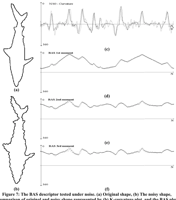
Total Score 2 83.16 82.62 79.92 77.14 69.38 86.12 87.27 One of the powers of the BAS descriptor comes from its insensitivity to noise. The behavior of the BAS descriptor under additive noise is investigated and compared to the K- curvature function plot. Figure 7 indicates the fish example distorted by additive noise. Note that the ripples appeared in the shape due to the noise, add additional peaks and valleys in the K-curvature function, if K is taken small enough to capture the ripples of the noise. The value of K should be large enough to smooth the noise and small enough to preserve the convexities and concavities of the context. On the other hand, the BAS descriptor smoothes the noise in the first order statistics, yielding almost the same plots for both the original and noisy images. The changes in the second and third moments are rather insignificant.

In most of the practical problems the noise deforms only a portion of the shape boundary. Since the BAS descriptor uses all other boundary points in calculation of beam angle statistics of each point, the additive noise applied to any part of the shape only slightly changes the beam angle statistics of the points.

(c)

(d)

(e) (a)

(b) (f)

Figure 7: The BAS descriptor tested under noise. (a) Original shape, (b) The noisy shape, Comparison of original and noisy shape represented by (b) K-curvature plot, and the BAS plot

(c) 1st moment (d) 2nd moment (e) 3rd moment.

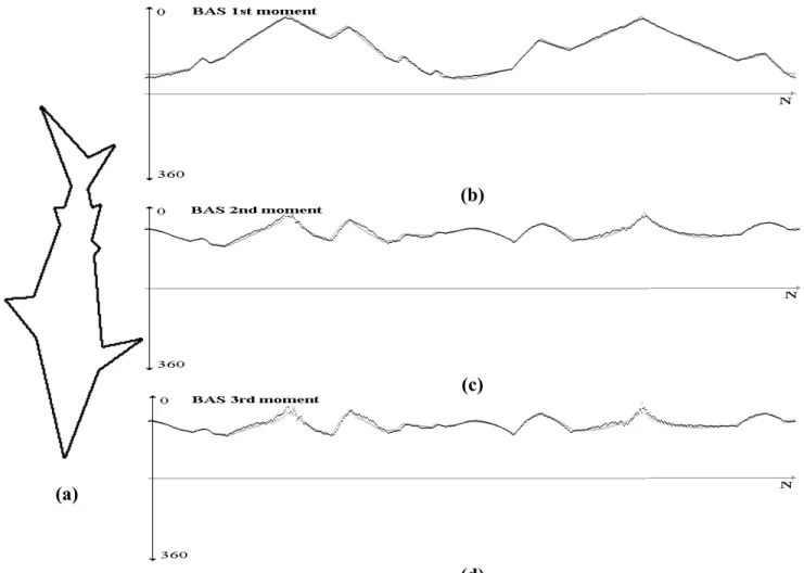
Conversely, the BAS descriptor is tested under smoothing effects. Curve evolution method (Latecki 2000.1) is used for smoothing and the BAS descriptor of the original shape and evolved shape is compared in figure 8. The degree of smoothing is decided by visual inspection, which preserves the maximal amount of context information. Note that, the BAS descriptor yields very similar first, second and third moments, indicating the scale independence of the proposed descriptor.

(b)

(c)

(a)

(d)

Figure 8: The BAS descriptor tested under smoothing effect. (a) The smoothed version of shape in Figure 7.a and its BAS plot (b) 1st moment (c) 2nd moment (d) 3rd moment.

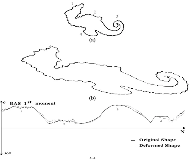
The experiments are performed in order to test the insensitivity of the BAS descriptor under shear and scale. Figure 9 shows the fish example distorted by shear. Note that the BAS descriptor is quite insensitive to shear transform, yielding almost the same first moment. Figure 9.c indicates the correspondence of each convex parts with the 2-D shape information (1st moment plot) yielding a consistent representation to the human visual system.

An important measure for the similarity based retrieval systems in large databases, is the time complexity of the overall algorithm. Time complexity of the proposed shape description scheme can be analyzed in two parts. The first part is the BAS representation, which requires the calculation of beam angle statistics for each boundary point. Since all the boundary points are used in BAS representation of each point, the time complexity of this algorithm is O(N2), where N is the number of boundary points. The second part is the similarity measurement, which finds the optimal correspondence of items in feature vectors. The time complexity of this algorithm is O(M2), where M is the number of entries in feature vectors. Since the starting point in boundary extraction is different for each shape, one of the feature vectors must be shifted in order to find the minimum distance between two shapes. This requires the computation of similarity distance for each shifted version of one feature vector. The overall time complexity of similarity measurement algorithm is O(M3).

(a)

(b)

(c)

Figure 9. a) A sample shape with major perceptual parts indicated by numbers 1 through 4 (b) the sheared and rescaled version c) The correspondence of visual parts and comparison of

two representations. 6. Conclusion

This study introduces a robust shape descriptor for identifying the similar objects in an image database. The two-dimensional object silhouettes are represented by one-dimensional BAS moment functions, which capture the perceptual information using the statistical information based on the beams of individual points. At each point, the angle between a pair of beams is calculated to extract the topological structure of the boundary. The representation avoids smoothing, in order to preserve all the available information in the shape. It also avoids the selection of a threshold value to represent the resolution of the boundary, thus eliminates the context-dependency of the representation to the data set. Therefore, rather than using a single representation of the boundary, at a predefined scale, the proposed descriptor uses the statistics of the representations at all scales. It gives globally discriminative features to each boundary point by using all other boundary points. It is simple and consistent with human perception through preserving the concave and convex parts of the shapes.

The experiments are done on the dataset of MPEG 7 Core Experiments Shape-1. The tests indicate that BAS descriptor is quite stable under distortions. It is insensitive to translation, rotation and scale. It is observed that the proposed shape descriptor outperforms the MPEG 7 shape descriptor.

In the proposed method, the BAS descriptor employs samples of the moment functions for the first three moments. This requires a feature vector with length of 3M, where M is the number of samples taken on the moment functions. The size of the feature vector can be reduced further if we can use only the points corresponding to only maxima and minima of the moments. The future work will be directed towards decreasing the space complexity of the BAS descriptor by finding more compact representation of the moment functions.

References

Agam, G., Dinstein, I., 1997. Geometric Separation Of Partially Overlapping Nonrigid Objects Applied to Automatic Choromosome Classification. IEEE Trans. PAMI, 19, 1212-1222.

Arica, N., Yarman-Vural F. T., 2002, A Perceptual Shape Descriptor. Proc. ICPR-2002 , 3, 375-378. Belongie, S., Malik, J., Puzicha, J., 2002. Shape Matching and Object Recognition Using Shape Contexts. IEEE Trans. PAMI, 24, 4, 509-522.

Chuang, G., Kuo, C. –C., 1996. Wavelet Descriptor of Planar Curves: Theory and Applications. IEEE Trans. Image Processing, 5, 56-70.

Cohen, F. S., Huang, Z., Yang, Z., 1995. Invariant Matching and Identification of Curves Using B-Splines Curve Representation. IEEE Trans. Image Processing, 4, 1-10.

Davis L. S., 1979. Shape Matching Using Relaxation Techniques. IEEE Trans. PAMI, 1, 60-72. Del Bimbo A., Pala, P., 1997. Visual Image Retrieval By Elastic Matching Of User Sketches. IEEE Trans. PAMI, 19, 121-132.

Khotanzan, A., Hong, Y. H., 1990. Invariant Image Recognition By Zernike Moments. IEEE Trans. PAMI, 12, 489-497.

Latecki, L. J., Lakamper, R., Eckhardt, U., 2000. Shape Descriptors for Nonrigid Shapes with a Single Closed Contour. Proc. IEEE Conf. CVPR, South Carolina.

Latecki, L. J., Lakamper, R., 2000.1. Shape Similarity Measure Based on Correspondence of Visual Parts. IEEE Trans. PAMI, 22, 10, 1185-1190.

Lin, L. –J., Kung, S. Y., 1996. Coding and Comparison of Dags as a Novel Neural Structure With Application To Online Handwritten Recognition. IEEE Trans. Signal Processing, .

Liu, H., Srinath, D., 1990. Partial Shape Classification Using Contour Matching in Distance Transformation. IEEE Trans. PAMI, 12, 1072-1079.

Loncaric, S., 1998. A survey of Shape Analysis Techniques. Pattern Recognition, 31, 983-1001. Mokhtarian, F., Mackworth, A., 1986. Scale Based Description and Recognition of Planar Curves and Two-Dimensional Shapes. IEEE Trans. PAMI, 8, 2-14.

Mokhtarian, F., Abbasi, S., Kittler, J., 1997. Efficient and Robust Retrieval By Shape Content Through Curvature Scale Space. Image Databases and Multimedia Search, A. W. M. smeulders and R. Jain ed., 51-58 World Scientific Publication.

Siddigi, K. Tresness, K. J., Kimia, B. B., 1996. Parts of Visual Form : Psychophysical Aspects. Perception, 25, 399-424.

Urdiales, C., Bandera, A., Sandoval, F., 2002. Non-parametric Planar Shape Representation Based on Adaptive Curvature Functions. Pattern Recognition, 35, 43-53.

Wang Y. P., Pavlidis T., 1990. Optimal Correspondence of String Subsequences. IEEE Trans. PAMI, 12, 1080-1087.