THE INVARIATOR DESIGN: AN UPDATE
L
UISM. C
RUZ-O
RIVE1 ANDX
IMOG
UAL-A
RNAUB
,21Department of Mathematics, Statistics and Computation, Faculty of Sciences, University of Cantabria, E-39005
Santander, Spain;2Department of Mathematics-INIT, University Jaume I, E-12071 Castell´o, Spain. e-mail: [email protected], [email protected]
(Received April 30, 2015; revised July 23, 2015; accepted September 21, 2015)
ABSTRACT
The invariator is a method to generate a test line within an isotropically oriented plane through a fixed point, in such a way that the test line is effectively motion invariant in three dimensional space. Generalizations exist for non Euclidean spaces. The invariator design is convenient to estimate surface area and volume simultaneously. In recent years a number of new results have appeared which call for an updated survey. We include two new estimators, namely the a posteriori weighting estimator for surface area and volume, and the peak-and-valley formula for surface area.
Keywords: invariator, peak-and-valley formula, stereology, surface area, test line weighting, volume.
INTRODUCTION
Since the publication of the invariator design (Cruz-Orive, 2005, although the name ‘invariator’ was first coined in Cruz-Orive, 2009b), a number of related papers have appeared with additional results – hence we thought that an update would now be opportune.
Briefly, the invariator design consists of two stages. In the first stage a randomly oriented plane, called the pivotal plane, is taken through a fixed point O, called the pivotal point. In the second stage a randomly oriented test line is sampled in the pivotal plane with a weight proportional to its distancer fromO. This test line is effectively equipped with the motion invariant density in space, whereby surface area and volume, for instance, can be estimated unbiasedly by design. The advantage of the invariator is that the necessary observations can be made solely in a pivotal plane which has to be randomly oriented, but not randomly located.
In the original paper the aforementioned r-weighting was made a priori, namely it was implicit in the design: each test line was drawn through a point from a UR grid on the pivotal plane, with a direction perpendicular to the axis joining the point withO. Here a new, more natural procedure, based on a posteriori r-weighting, is proposed which requires only a system of parallel test lines (SectionTest lines with a posteriori weighting).
In Cruz-Orive (2005) a method was also proposed to estimate the surface area of a convex object by measuring Feret rays emanating from O in a pivotal section. Recently, Th´orisd´ottir and Kiderlen (2014) have generalized the result to non convex objects, see
also Th´orisd´ottir et al. (2014). Following a different approach, Gual-Arnau and Cruz-Orive (2015) have obtained a simplified version of the relevant estimator, see Section Case of a general object: the peak-and-valley formula.
To make the survey widely accessible, an informal description of concepts like ‘invariant density’ is given in the next section. For completeness, elementary proofs of relevant stereological results are given in the appendixes.
PREREQUISITES AND NOTATION
Here we introduce basic tools of integral geometry (Santal´o, 1976; De-Lin, 1994) for geometric sampling. We concentrate on points, straight lines and planes to be used as test probes, namely on geometric elements equipped with a well defined mechanism of randomness, used to probe (namely to hit, or intersect, with a sampling purpose) a target subset in Euclidean space.
µ(Y) = Z
Y
µ(dx) (1)
does not depend on the choice of the origin of abscissas. The preceding integral may be interpreted as the measure of points inY. Here we consider a measure element µ(dx) associated with the length element dx which may be expressed as µ(dx) =w(x)dx, where w(x)is a non negative weight function. The problem is to findw(x)such that, for any translation vectorz∈R1, the identity
Z
Y
w(x)dx=
Z
Y+z
w(x)dx (2)
holds, where Y +z represents the translate of the intervalY by the vectorz. In the left hand side integral make the change of variablex=y−z. Then,
Z
Y
w(x)dx=
Z
Y+z
w(y−z)dy. (3)
The right hand sides of the preceding two identities must coincide for all z∈R1. Thus, for each x ∈R1 we must have thatw(x) =w(x−z)for allz∈R1, (up to a set of points of zero length), which implies that w(x) =constant. The constant is a scale factor that may be taken to be equal to 1, and therefore the translation invariant element of measure for points in R1 is the length element,
µ(dx) =dx. (4) In integral geometry, a motion invariant measure element such as the preceding one is usually called a motion invariant density. Any such density is always taken in absolute value because it must be non negative.
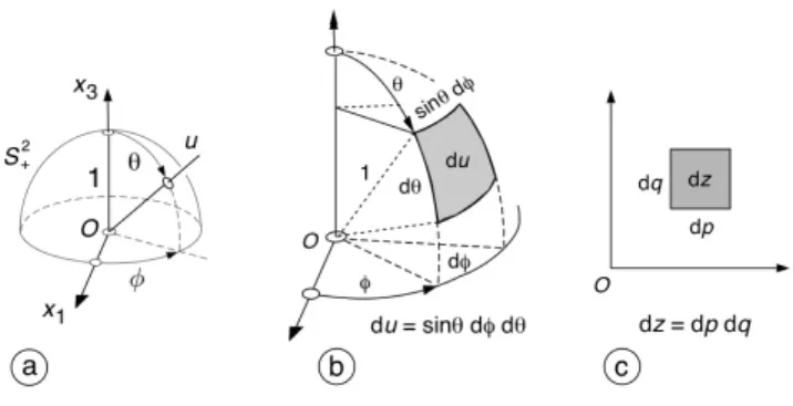
Similarly, the translation invariant density of a point in Rd is the d-dimensional volume element (namely the Lebesgue measure element) in Rd, see Fig. 1a and Fig. 2c. Hence, in this case µ(Y) is the volume of Y, which does clearly not depend on the location and orientation ofY.
A test probe equipped with the motion invariant density is called an invariant probe, for short. Henceforth the pertinent invariant densities are given without proof, which can be found for instance in the aforementioned books.
For coherence with the sequel a point of abscissa p on an arbitrary axis (i.e. onR1) may be denoted by L10≡L10(p). Its translation invariant density is
dL10=dp, (5)
as we have seen. From a statistical viewpoint, the probability that a point endowed with the preceding
invariant density belongs to an interval of length dx, given that the pointxbelongs to an interval of length h > 0, is equal to the ratio of the corresponding measures, namely dx/h. This is the probability element of a uniform random (UR) variable in an interval of length h >0. Therefore, a point endowed with the invariant density, and belonging to any bounded interval of the real axis, is UR in that interval.
Fix a rectangular frame with originOin the plane R2. An axisL21[0]of directionφ∈[0,π)is a unoriented straight line through O (hence the subscript ’[0]’) making an angle φ with the positive half axis of abscissas. This is equivalent to joiningOwith a pointφ of the unit semicircleS1+. The rotation invariant density
of an axis is,
dL21[0]=dφ, (6)
namely the length element in S1+, see Fig. 1b. Thus, φ is uniform random (UR) in any interval of the semicircle. In geometric sampling, an axis equipped with the rotation invariant density is said to be isotropic random (IR).
A straight line L21 ≡L21(p,φ) in R2 is normal to an axis L21[0] of direction φ, called the orthogonal complement of the line, at a signed distance p ∈ (−∞,∞)fromO. The pair(p,φ)are called the normal coordinates of L21, see Fig. 1c. The motion invariant density ofL21, namely the density invariant with respect to rotations and translations, is,
dL21=dpdφ. (7)
It is equivalent to takep∈[0,∞)andφ∈[0,2π).
Because the orientation of an invariant line is IR, and its translation parameter pis UR in any bounded interval of the orthogonal complement of the line, an invariant test line hitting a bounded subset of the plane is said to be isotropic uniform random (IUR) hitting the subset (Miles and Davy, 1976). The latter term applies to any invariant probe hitting a target subset in any dimension.
Fix a rectangular trihedron with originOin space R3. An axisL31[0]≡L31(0,u)of directionu≡u(φ,θ)∈ S2+ is a unoriented straight line joining O with a
point u of the unit hemisphere S2+, see Fig. 2a. The
angles(φ,θ) are the spherical polar coordinates ofu, namely the longitude φ ∈[0,2π), and the colatitude θ ∈[0,π/2]. The rotation invariant density of an IR axis is,
dL31[0]=du=sinθdφdθ, (8)
namely the area element inS2+, see Fig. 2b. Thus,uis
UR in any region of the hemisphere.
The rotation invariant density of an IR plane L32[0] ≡L32(0,u) through O is equal to du, namely the same as the invariant density of its normal axis L31(0,u).
The plane L32 ≡ L32(p,u) is parallel to L32(0,u) at a distance p ∈ (−∞,∞) from O, see Fig. 3a.
Equivalently, L32(p,u) is a translate of the plane L32(0,u) by a distance p along the orthogonal complementL31(0,u). The motion invariant density of L32is,
dL32=dpdu. (9)
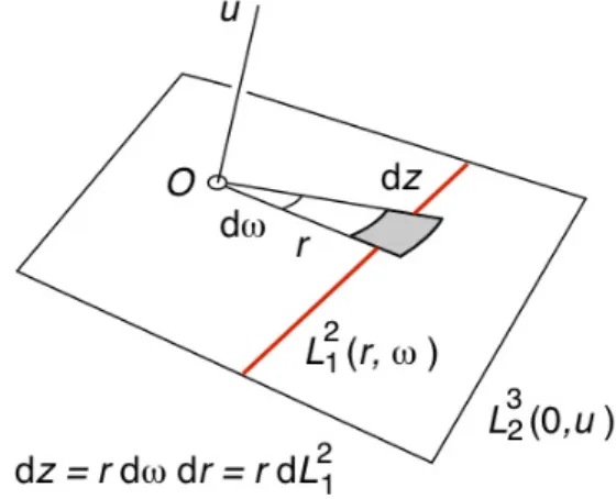
A straight line L31≡L31(z,u) in R3 is a translate of the axis L31(0,u) to a point z in the orthogonal complement of the line, namely in the perpendicular plane L32(0,u), see Fig. 3b. The motion invariant density ofL31is,
dL31=dzdu. (10)
In turn, if (p,q) denote the Cartesian coordinates ofzinL32(0,u), then,
dz=dpdq, (11)
(Fig. 2c), namely the motion invariant density for points in L32(0,u). Thus the point z is UR in any bounded region of the latter plane.
Fig. 2. (a) Axial direction through a point u of the unit hemisphere. (b) The rotation invariant density for a direction u in three dimensional space is the area element du on the unit hemisphere. (c) The motion invariant density for a point z in the plane is the area elementdz.
Fig. 3. (a) Parametrization of a plane. (b) Parametrization of a straight line.
THE INVARIATOR DESIGN
CLASSICAL CROFTON INTERSECTION FORMULAE FOR SURFACE AREA AND VOLUME
The object of interest is a fixed, bounded, nonvoid subset Y of three dimensional Euclidean space R3, (often said ‘in 3D’), with piecewise smooth boundary ∂Y. The target parameters are the volumeV ofY, and the surface areaSof∂Y.
The geometric probe adopted here to estimate S andV is an IUR test lineL31≡L31(z,u)hittingY. The classical representations of S and V in terms of the intersection measure of an IUR test line hittingY are given by the following Crofton formulae (for a cursory derivation see Appendix I):
S= 1 π
Z
V = 1 2π
Z
L(Y∩L31)dL31, (13)
where the density dL13 is given by Eq. 10, and I(·), L(·) denote intersection number and intercept length, respectively, with I(/0) =L(/0) =0. The integrals are extended to the following set,
{(z,u) : z∈L32(0,u),u∈S2+}, (14)
whereL32(0,u) denotes the orthogonal complement of the test lineL31(z,u).
The preceding identities underlie the classical isotropic sampling designs. An invariant line L31 is normal to an IR planeL32[0]≡L32(0,u) at an invariant point z in that plane. This principle leads to the fakir probe, see for instance Fig. 1a from Cruz-Orive et al. (2010). It can be shown that an equivalent procedure is to take an invariant plane L32 (not just an IR plane L32[0]), and then an invariant test line withinL32. This leads to the isotropic Cavalieri design with test lines, see for instance Fig. 3 from the latter paper. Both designs therefore require translating test lines in 3D. The invariator principle, however, establishes that an invariant test line L31 can be effectively generated within an isotropic plane L2[0]3 . This requires translating test lines in 2D, which constitutes a practical advantage.
THE INVARIATOR PRINCIPLE
The ensuing approach, and the mathematical derivations given in the appendixes, are somewhat informal – for a more rigorous treatment see Gual-Arnau and Cruz-Orive (2009), Auneau and Jensen (2010), Gual-Arnauet al.(2010), and Th´orisd´ottir and Kiderlen (2014). The idea was first developed in Cruz-Orive (2005), and it was inspired by a result of Varga (1935, Eq. 10). It is noteworthy that the key density decomposition – see Eq. 16 below – appeared in Jensen and Gundersen (1989, Eq. 5.35), but its potential was not exploited further. Schneider and Weil (2008, p. 285) indicate that the mentioned decomposition is related with a general result of Petkantschin (1936). In any case, the relevance of the invariator lies mainly in the practical ramifications of a simple principle.
Recall that the invariant density dL31of a test lineL31 in 3D is given by Eq. 10 as the product of the invariant density dzof a pointzin the planeL32[0]orthogonal to the line, times the invariant density du of that plane. In the invariator context the IR planeL32[0] is called the ‘pivotal plane’, because it is a plane through a fixed pointOand free to rotate or ‘pivot’ in space aroundO.
The density dzmay be expressed in polar coordinates (r,ω)as follows,
dz=rdrdω r∈[0,∞),ω∈[0,2π). (15) Thus, dL31may be decomposed as follows,
dL31=rdrdωdu=rdL21du, (16) where dL12 = drdω is the invariant density of a straight line in the plane (Eq. 7). The preceding decomposition is valid provided that the orthogonality of the geometric elements involved is preserved, that is, the distance r must be measured along an axis perpendicular to L21 within the pivotal plane L32[0] (Fig. 4). Moreover, the angle ω is measured in the pivotal plane, and therefore the line L21 must also be contained in the pivotal plane at a distancer fromO. The preceding construction is the invariator principle.
Fig. 4.Scheme of the invariator principle.
With the invariator principle the classical Eqs. 12, 13 become the invariator equations,
S= 1 π
Z
dL32[0]
Z
r·I
n
∂Y∩L32[0]
∩L21
o
dL21,
(17)
V = 1 2π
Z
dL32[0]
Z
r·L
n
Y∩L32[0]
∩L21
o
dL21,
(18)
respectively. The outer integral is extended over the unit hemisphereS2+, whereas, for each directionu of
the pivotal planeL32[0] ≡L32(0,u), the inner integral is extended to the parameter space
{(r,ω) : r∈[0,∞),ω∈[0,2π)} (19)
test line directly in 3D, as it was the case for Eqs. 12, 13, with the invariator designY is first hit by a pivotal plane, and then the pivotal section is in turn hit by an invariant test line in the pivotal plane. Note also that the distance factor ‘r’ appears in the integrand.
Eq. 18 may be written,
V = 1 2π
Z α
Y∩L32[0]
dL32[0], (20)
where
α(Y∩L32[0]) =
Z
r·L
n
Y∩L32[0]
∩L21
o
dL21 (21)
is a functional depending on the pivotal sectionY ∩ L32[0]only – and similarly for Eq. 17.
As explained in the following sections, conditional on a given IR direction u∈S2+ of the pivotal plane,
Eqs. 17, 18 give rise to a variety of different unbiased estimators ofSandV. Translated to the present special cases, however, Conjecture 4.1 from Gual-Arnau et al. (2010) says that, conditional on a given pivotal section, the averages of all possible estimators of V will always boil down to Eq. 21 up to a constant factor, and analogously forS. In other words, ifψ1(u),ψ2(u)
are the averages of any two unbiased estimators ofV defined on a pivotal planeL32(0,u), namely if
1 2π
Z
ψ1(u)du=
1 2π
Z
ψ2(u)du=V , (22)
then the conjecture implies thatψ1(u) =ψ2(u)for all
u∈S2+, and similarly for S. (Note that, in general, if
two integrals coincide, the corresponding integrands do not need to coincide).
In Cruz-Orive (2012) the preceding conjecture was proved on the one hand for the different invariator estimators given below for the volume V of an arbitrarily shaped objectY, and on the other hand for the surfactor estimator of the surface areaSof a convex bodyY, (Jensen and Gundersen 1987, 1989). (Recall thatY is convex if the straight line segment joining any two points ofY, lies entirely in Y). The general conjecture remains open, however, partly because the examined estimators need not be the only possible ones.
It should be stressed that for a finite number of linear probes generated in a pivotal section, the volume estimators given below are different, even though their means will always coincide for any given pivotal section, and similarly for the surface area estimators. Consequently, the estimators will generally have different variances under similar sampling intensities - for an illustration of this see Cruz-Orive (2008).
INVARIATOR ESTIMATORS OF
SURFACE AREA AND VOLUME
USING TEST LINES
The estimators given in the next subsection emerge directly from Eqs. 17, 18. A pivotal section is hit by an invariant test line with density dL21in the pivotal plane, and the pertinent measures (I(·), orL(·), respectively) are weighted a posteriori for each test line, namely multiplied by the distancer from the pivotal pointO to the test line.
On the other hand, the estimators given in the second subsection below use the fact that the factor rdL21 in the integrand of the mentioned equations is the invariant density dz of a point in the pivotal plane (Eq. 15). Thus, a UR grid of points may be generated in the pivotal plane and then a test line is drawn through each grid point perpendicular to the axis joining the pivotal pointOwith the grid point. In this way the factor r is implicit in the UR generation of the grid, which means that each test line is weighted automatically by the sampling design. Such test line, which we denote by L21[·] ≡L21[·](z) may be called a pivotal test line and, as indicated above, its invariant density
dL21[·](z) =rdL21(r,ω) =dz, (23)
is that of the pointz. The corresponding grid may be called a pivotal grid, see Cruz-Orive (2009a). Thus, for the a priori weighted design the invariator Eqs. 17, 18 take the following form,
S= 1 π
Z
dL32[0]
Z
I
n
∂Y∩L2[0]3
∩L21[·]
o
dL21[·],
(24)
V = 1 2π
Z
dL32[0]
Z
L
n
Y∩L32[0]
∩L21[·]
o
dL21[·].
(25)
TEST LINES WITH A POSTERIORI WEIGHTING
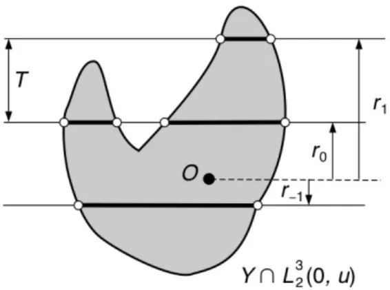
On a pivotal plane L32(0,u) generate a UR grid of parallel test lines a distance T >0 apart with IR orientationω ∈[0,π), namely,
L21(rk,ω),k∈Z , (26) where
rk= (U1+k)T, ω =U2π, (27) denote the signed distance from the pivotal pointOto thekth test line of the grid, and the orientation of the normal to the test line, respectively, whereas U1, U2
are two independent UR numbers in the interval[0,1), (Fig. 5). Set,
Ik=I
∂Y∩L32(0,u)
∩L21(rk,ω) ,
Lk=L
Y∩L32(0,u)∩L12(rk,ω) .
(28)
Then, (Appendix II),
b
S=2πT
∑
k∈Z
|rk|Ik, (29)
b
V =πT
∑
k∈Z
|rk|Lk, (30)
are unbiased estimators (UE) ofSandV, respectively.
To increase precision two mutually perpendicular IUR grids of parallel test lines may be generated on the pivotal plane, whereby the summations in the right hand sides of the preceding two equations should be replaced with their corresponding averages.
Fig. 5. Illustration of the a posteriori weighting method to estimate S and V using Eqs. 29 and 30 respectively. The parallel test lines are IUR hitting the pivotal section – here they are shown horizontal for convenience. The relevant intersections are marked with white dots, the relevant intercepts with thick line segments. Here I−1 = 2, I0 = 4, I1 = 2. The
intercept lengths and their distances from a parallel axis through the pivotal point O have to be measured at the specimen scale.
TEST LINES WITH A PRIORI WEIGHTING
On the pivotal planeL32(0,u)generate a UR square grid of test points of sizeT >0, namely,
zi j= ((U1+i)T,(U2+j)T),i,j∈Z . (31)
LetL21[·](zi j)represent a pivotal line, namely a test
line through the point zi j in the pivotal plane, and
normal to the axis joining the pivotal pointOwithzi j,
see Fig. 6. Then
n
L21[·](zi j),i,j∈Z
o
(32)
a pivotal grid. Set,
I=
∑
i∈Zj
∑
∈ZI
n
∂Y∩L32(0,u)∩L21[·](zi j)
o
L=
∑
i∈Zj
∑
∈ZL
n
Y∩L32(0,u)∩L21[·](zi j)
o .
(33)
namely the total number of intersections and the total intercept length, respectively, determined by the pivotal grid in the pivotal section.
Then (Appendix III),
b
S=2aI, (34)
b
V =aL, (35)
wherea=T2, are unbiased estimators (UE) of Sand V, respectively (Cruz-Orive, 2005).
Recall that the invariant density of a pivotal line is that of a point. Therefore a pivotal line is not an invariant test line in the pivotal plane, but it is so in 3D by virtue of the invariator principle. Thus, not surprisingly the preceding estimators are identical to those corresponding to the isotropic fakir probe (Cruz-Orive, 2013, Section 5).
INVARIATOR ESTIMATORS OF
VOLUME ONLY
The estimators given below are not recent – for instance the integrated nucleator was already described in (Jensen, 1991; 1998) and applied in Hansen et al. (2011), whereas the nucleator was described in Gundersen (1988). They are included here, however, because they also emerge from Eq. 18, (for general accounts see Jensen and Rataj, 2008; Auneau and Jensen, 2010; Gual-Arnauet al., 2010).
The ordinary version of the integrated nucleator is defined on a pivotal section, and it is based on the following representation,
V = 1 π
Z
S2+ du
Z
Y∩L3 2(0,u)
ρ(z,u)dz, (36)
(Appendix IV), where ρ(z,u) denotes the absolute distance from the pivotal pointO to a point z of the pivotal section. It is assumed thatO∈Y. In the next subsection, the corresponding volume estimator based on a sample of points in the pivotal section is called the discretized nucleator.
The initial idea underlying the nucleator (Cruz-Orive, 1987, Appendix B), was based on a ray emanating from a fixed pointOdirectly in 3D space, namely in a direction u ∈ S2. If such ray hits the sampled objectY, then the corresponding intersection will in general consist of say m(u) ≥ 1 separate intercept segments. The distances of the end points of these intercepts fromO, arranged in increasing order of magnitude, may be denoted as follows,
{li−(u),li+(u);i=1,2, . . . ,m(u)} . (37)
Then the direct 3D nucleator estimator stems from the following integral,
V =1 3
Z
S2
m(u)
∑
i=1
li3+(u)−li3−(u)du. (38)
IfO∈Y, thenl1−(u) =0 for allu. If the objectY
is moreover star convex with respect toO∈Y, namely if the ray joiningOwith any point of the boundary∂Y is always simply connected, then
V= 1 3
Z
S2
l+3(u)du. (39)
where l+(u) ≡ l1+(u) is the intercept length
determined by a ray in the directionu.
The nucleator version stemming from the invariator Eq. 18, however, is a two stage one. In the first stage an IR pivotal plane is generated through the pivotal pointOand then, in the second stage an IR ray emanating fromOis generated within the pivotal plane making an IR angleϕin[0,2π)with a fixed half axis in the pivotal plane. Thus – assuming for the clarity of exposition thatY is star convex with respect toO∈Y – the relevant integral now is,
V = 1 3π
Z
S2+ du
Z 2π
0
l+3(ϕ;u)dϕ, (40)
(Appendix IV). As opposed to the direct nucleator (Eq. 39), the preceding version may be called the pivotal nucleator.
The two nucleator estimators stemming directly from Eqs. 39 and 40 will be clearly unbiased, but not identical, and they will generally not share the same precision for a fixed sample size of n rays, say. Note that in the direct nucleator thenrays may be sampled according to a pseudosystematic design directly on the unit sphere and they will not be coplanar in general (Gual-Arnau and Cruz-Orive, 2002), whereas in the pivotal nucleator the n rays will be sampled on the unit circle within a pivotal section. In practice, the nucleator has generally been applied as a two stage procedure, whereby a pivotal section (either isotropic, or vertical) is sampled first, and then the rays are sampled in that section (Gundersen, 1988).
THE DISCRETIZED NUCLEATOR
{z1,z2, . . . ,zn}. Let di ≥0 denote the distance of the
hitting grid pointzifromO(Fig. 7a). Then,
b
V =2a
n
∑
i=1
di, (41)
wherea=T2, is an UE ofV.
THE PIVOTAL SECTION NUCLEATOR
On the pivotal planeL32(0,u)generatensystematic rays an angle 2π/napart, emanating from the pivotal point O. Thus the angles made by the n rays with a fixed half axis in the pivotal plane are,
ϕk= (U+k)·
2π
n ,k=1,2, . . . ,n
, (42)
whereUis a UR number in the interval[0,1).
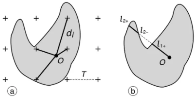
Fig. 7. (a) Illustration of the discretized nucleator, Eq. 41, (n=4 distances are generated). (b) Idem of the pivotal nucleator with a single ray,(n=1,m1=2),
Eq. 44.
If thek-th ray hits the sampled objectY, then the corresponding intersection will consist of saymk ≥1
separate intercepts. The distances of the end points of these intercepts from O, in increasing order of magnitude, are denoted as follows,
lk,i−,lk,i+; i=1,2, . . . ,mk , (43)
(Fig. 7b). If O ∈Y, then lk,1− = 0 for all k. The
nucleator estimator defined on a pivotal section Y∩ L32(0,u)reads
b
V =4π 3n
n
∑
k=1
mk
∑
i=1
lk3,i+−lk3,i−, (44)
and it is unbiased forV.
IfY is star convex with respect to a pivotal point O∈Y, namely if the intersection betweenY and any ray emanating fromOis always simply connected for any pivotal section, then
b
V =4π 3n
n
∑
k=1
lk3,+, (45)
wherelk,+≡lk,1+is the intercept length determined by
thekth ray in the pivotal section.
INVARIATOR ESTIMATORS OF
SURFACE AREA ONLY
CASE OF A CONVEX OBJECT: THE FLOWER FORMULA
In Cruz-Orive (2005) an invariator estimator of surface area, thereafter known as the flower estimator (Cruz-Orive, 2011; Dvoˇr´ak and Jensen, 2013), was obtained from Eq. 24 for the special case in which the object Y is a convex body. Clearly, in this case the intersection number I
n
∂Y∩L32[0]
∩L21[·](z)o is equal to 2 almost surely (namely with probability 1) whenever the pivotal test line L21[·](z) hits the pivotal section, and equal to 0 otherwise. Equivalently, the hitting event takes place whenever the pointzbelongs to a setHY∩L3
2[0]called the support set or ‘flower’ of the pivotal section with respect to the pivotal pointO. The boundary∂HKof the flowerHK of a convex setKwith
respect to a fixed point O, is the geometric locus of the intersection between a variable tangent to∂K and the normal to this tangent fromO, see Fig. 8. In other words,∂HKis the pedal curve of∂Kwith respect toO,
see for instance Lockwood (1961). Thus, in this case Eq. 24 becomes the flower formula:
S=4
Z
S2+ du 2π
Z
H
Y∩L3 2[0]
dz
=4Eu
A
HY∩L3 2[0]
,
(46)
Fig. 8.(a) Pivotal section (red boundary) of a convex body Y . (b) Flower of the pivotal section.
Leth(ω),(0≤ω<2π)denote the radial function of the flower with respect to an interior pivotal point O∈Y. Then the flower formula may be written,
S=4Eu
1 2
Z 2π
0
h2(ω)dω
. (47)
On the pivotal plane generate n systematic rays an angle 2π/n apart emanating from O, as in the pivotal nucleator design. Measure the corresponding radial lengths {hk+,k=1,2, . . . ,n} of the flower, or
equivalently the ‘Feret rays’ of the pivotal section. Then an UE of the surface area of a convex body is,
b
S= 4π n
n
∑
k=1
h2k+, (48)
which may be regarded as a companion of Eq. 45 when Y is convex. In Cruz-Orive (2005) the choice n=4 was recommended. Later, Dvoˇr´ak and Jensen (2013) discovered certain optimality properties of this choice as far as estimation precision is concerned.
CASE OF A GENERAL OBJECT: THE PEAK-AND-VALLEY FORMULA
For a non convex object Y an adaptation of the flower formula is possible starting from Eq. 17. Let C≡∂Y∩L32(0,u)represent the pivotal trace curve. The main task is to identify the number of intersections I(C∩L21(r,ω)) in terms of (r,ω). For each direction angle ω ∈[0,2π) consider a line L21(r,ω) sweeping the pivotal plane parallel to itself fromr= +∞down to r =0, in search of critical points of the height function restricted to the curveCin the given direction. In general, a critical point may be a local maximum, or minimum, with a tangent, or a local supremum, or infimum, without a tangent. To include all cases a local maximum, or supremum, will be called a peak,
whereas a local minimum, or infimum, will be called a valley. IfChas points above the axis L21(0,ω), then we assign an index εk = +1 if the kth critical point
encountered is a peak, and εk =−1 if it is a valley.
The first critical point is necessarily a peak, the second is also a peak if C is not convex. Thus, ε1 =ε2 =
+1. Thereafter the critical point may be a peak, or a valley. Immediately after a peak is met, two new intersections appear whereas, after a valley is met, two intersections are lost. Suppose thatmcritical points are met successively, and let h1>h2> . . .hm>hm+1 ≡
0 denote their corresponding distances from the axis L21(0,ω). Then,
I(C∩L21(r,ω)) =
0, r>h1,
2=2ε1, r∈(h2,h1],
4=2(ε1+ε2), r∈(h3,h2],
. . . , . . .
2∑mi=1εi, r∈(hm+1,hm].
(49) Naturally mand {(εk,hk),k=1,2, . . . ,m} depend on
(u,ω)in general. Now Eq. 17 yields (Gual-Arnau and Cruz-Orive, 2015),
S= 1 π Z
S2+ du
Z 2π
0 dω
m
∑
k=1 Z hk
hk+1
2
k
∑
i=1 εi
!
rdr
= 1 π Z
S2+ du
Z 2π
0
dω
m
∑
k=1
(h2k−h2k+1)
k
∑
i=1 εi
= 1 π Z
S2+ du
Z 2π
0
dω
m
∑
k=1 εkh2k .
(50)
From the preceding result a UE of S – called the peak-and-valley estimator – follows, namely,
b
S=4π
m
∑
k=1
εkh2k , (51)
(with Sb=0 if m=0) which is based on a single IR
direction angleω∈[0,2π)of the sweeping line in a IR pivotal plane of directionu∈S2+. To increase precision
a numbernof systematic orientations may be sampled on the pivotal plane, whereby the right hand side of Eq. 51 should be replaced with the corresponding average. If the target objectY is convex and O∈Y, then the preceding estimator reduces to Eq. 48. Note, however, that the general estimator is also valid for O∈/Y.
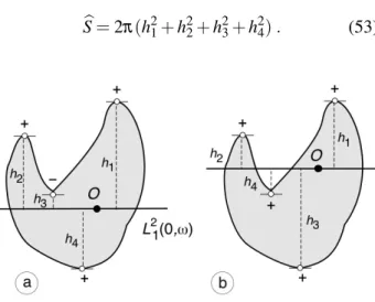
Example. Fig. 9a represents a pivotal trace C≡ ∂Y∩L32(0,u)determined in the boundary of the target object Y by a pivotal plane L32(0,u) through a fixed pivotal point O previously identifiable in Y, (e.g. a nucleolus of a neuron). The axisL21(0,ω)in the pivotal plane has been conveniently oriented as horizontal, but it is supposed to be isotropically oriented about O. In Fig. 9b the section is the same but, for the sake of illustration, the pivotal point has a different location relative toY. A sweeping lineL21(r,ω)moves parallel toL21(0,ω)from top to bottom. Instead of considering thatrvaries from+∞to 0 for eachω∈[0,2π), which was convenient to derive the result (50), in practice it is convenient to consider that r varies from+∞to
−∞ for each ω ∈[0,π). It then suffices to replace the factor 4 with 2 in the right hand side of Eq. 51. Thus the lineL21(r,ω)sweeps the traceCentirely from top to bottom for each sampled orientation angleω∈ [0,π). Below the axis L21(0,ω), however, it is useful to imagine the pivotal trace rotated by an angle of 180o and use the same criterion to identify peaks and valleys. In this mannerm=4 critical points are met in each case. In Fig. 9a the third critical point is a valley, wherebyε3=−1. The remaining three critical points
are peaks, henceε1=ε2=ε4= +1. Thus, in this case
an unbiased estimate ofSwould be,
b
S=2π(h21+h22−h23+h24). (52)
In Fig. 9b, however, the four critical points are all peaks, whereby, in this case,
b
S=2π(h21+h22+h23+h24). (53)
Fig. 9. Illustration of the peak-and-valley method to estimate S from a pivotal section. See text.
DISCUSSION
As mentioned in the SectionThe invariator design, the various estimators described here for volume
coincide in the mean for each pivotal section. For a finite sample of test lines, however, the estimators will have different variances in general. Apart from the empirical study carried out in Cruz-Orive et al. (2010) and the synthetic ones of Cruz-Orive (2008) and Dvoˇr´ak and Jensen (2013), little is known about the variance of the different estimators. Moreover, variance prediction formulae from a single sample will be precluded in practice whenever a single pivotal section is available. There is therefore scope for further research in this area. The same can be said for the invariator estimator of surface area, which coincides in the mean (for each pivotal section) with the surfactor at least for convex objects (Cruz-Orive, 2012).
The distinction between a priori and a posteriori weighting (SectionsThe invariator design,Invariator estimators of surface area and volume using test lines) deserves further comments.
(a) An a priori weighted test line L21[·] in a pivotal plane is effectively a motion invariant test line in 3D. On the contrary, a posteriori weighting uses a test lineL21 which is motion invariant in the pivotal plane, but not in 3D. For this reason, a factor ‘r’ has to be inserted in the integrand of Eqs. 17, 18 – this means “a posteriori weighting”.
(b) Because a weighted test lineL21[·] is effectively motion invariant in 3D, it will sample intercept lengths directly from the corresponding intercept length distribution of a given object. Since the latter distribution depends only on the object, the variance of the estimator given by Eq. 35 will not depend on the location of the pivotal point (Cruz-Orive, 2008). On the contrary the variance of the nucleator, for instance, will depend on that location. For an illustration of this fact see Fig. 7 from the latter paper.
Regarding the peak-and-valley formula to estimate surface area, it is noteworthy that the critical points of the pivotal trace do not need to have a tangent. Since we have supposed that∂Y is a piecewise smooth surface, the pivotal trace C might be a piecewise smooth curve, and therefore the critical points of its height function might not be defined for every direction. For instance, the third critical point in Fig. 9a is a valley with no tangent, but this is of no consequence for the estimator given by Eq. 51.
ACKNOWLEDGEMENTS
The second author acknowledges financial support from the UJI project P11B2012-24 and the PROMETEOII/2014/062 project.
REFERENCES
Auneau J, Jensen EBV (2010). Expressing intrinsic volumes as rotational integrals. Adv Appl Math 45:1–11. Cruz-Orive LM (1987). Particle number can be estimated
using a disector of unknown thickness: the selector. J Microsc 145:121–142.
Cruz-Orive LM (2002). Stereology: meeting point of integral geometry, probability, and statistics, Mathematicae Notae. In memory of Professor Luis A. Santal´o (1911–2001). 41:49–98.
Cruz-Orive LM (2005). A new stereological principle for test lines in 3D. J Microsc 219:18–28.
Cruz-Orive LM (2008). Comparative precision of the pivotal estimators of particle size. Image Anal Stereol 27:17– 22.
Cruz-Orive LM (2009a). The pivotal tessellation. Image Anal Stereol 28:101–05.
Cruz-Orive LM (2009b). Stereology: old and new, In: Capasso V, Aletti G, Micheletti A, eds. Proc 10th Eur Congr Stereol Image Anal. Bologna: Esculapio. Cruz-Orive LM (2011). Flowers and wedges for the
stereology of particles. J Microsc 243:86–102.
Cruz-Orive LM (2012). Uniqueness properties of the invariator, leading to simple computations. Image Anal Stereol 31:87–96.
Cruz-Orive LM (2013). Variance predictors for isotropic geometric sampling, with applications in forestry. Stat Methods Appl 22:3–31.
Cruz-Orive LM, Ramos-Herrera ML, Artacho-Perula E (2010). Stereology of isolated objects with the invariator. J Microsc 240:94–110.
De-Lin R (1994). Topics in integral geometry. Singapore: World Scientific.
Dvoˇr´ak J, Jensen EBV (2013). On semiautomatic estimation of surface area. J Microsc 250:142–57.
Gual-Arnau X, Cruz-Orive LM (2002). Variance prediction for pseudosystematic sampling on the sphere. Adv Appl Prob 34:469–83.
Gual-Arnau X, Cruz-Orive LM (2009). A new expression for the density of totally geodesic submanifolds in space forms, with stereological applications. Diff Geom Appl 27:124–28.
Gual-Arnau X, Cruz-Orive LM (2015). New rotational integrals in space forms, with an application to surface area estimation. Appl Math-Czech. To appear.
Gual-Arnau X, Cruz-Orive LM, Nu˜no-Ballesteros JJ (2010). A new rotational integral formula for intrinsic volumes in space forms. Adv Appl Math 44:298–308.
Gundersen HJG (1988). The nucleator. J Microsc 151:3–21. Hansen LV, Nyengaard JR, Andersen JB, Jensen EBV (2011). The semi-automatic nucleator. J Microsc 242:206–15.
Jensen EBV (1991). Recent developments in the stereological analysis of particles. Ann Inst Statist Math 43:455–68.
Jensen EBV(1998). Local stereology. Singapore: World Scientific.
Jensen EBV, Gundersen HJG (1987). Stereological estimation of surface area of arbitrary particles. Acta Stereol 6 (Suppl. III):25–30.
Jensen EBV, Gundersen HJG (1989). Fundamental stereological formulae based on isotropically orientated probes through fixed points with applications to particle analysis. J Microsc 153:249–67.
Jensen EBV, Rataj J (2008). A rotational integral formula for intrinsic volumes. Adv Appl Math 41:530–60. Lockwood EH (1961). A book of curves. Cambridge:
Cambridge University Press.
Miles RE, Davy PJ (1976). Precise and general conditions for the validity of a comprehensive set of stereological fundamental formulae. J Microsc 107:211–26.
Petkantschin P (1936). Zusammenh¨ange zwischen den Dichten der linearen Unterr¨aume im n-dimensionalen Raum. Abh Math Sem Hamburg 11:249–310.
Santal´o LA (1976). Integral geometry and geometric probability. Addison-Wesley, Reading, Massachusetts. Schneider R, Weil W (2008). Stochastic and integral
geometry. Berlin: Springer-Verlag.
Th´orisd´ottir O, Kiderlen M (2014). The invariator principle in convex geometry. Adv Appl Math 58:63–87. Th´orisd´ottir O, Rafati AH, Kiderlen M (2014). Estimating
the surface area of nonconvex particles from central planar sections. J Microsc 255:49–64.
Varga O (1935). Integralgeometrie 3. Croftons Formeln f¨ur den Raum. Math Z 40:387–405.
APPENDIX I: CROFTON
INTERSECTION FORMULAE
The volume element determined in the object Y by a test line L31(z,u) of fixed orientation u ∈ S2+
is dv(z,u) =L Y∩L31(z,u)dz. Integration over the domain given by Eq. 14 yields Eq. 13.
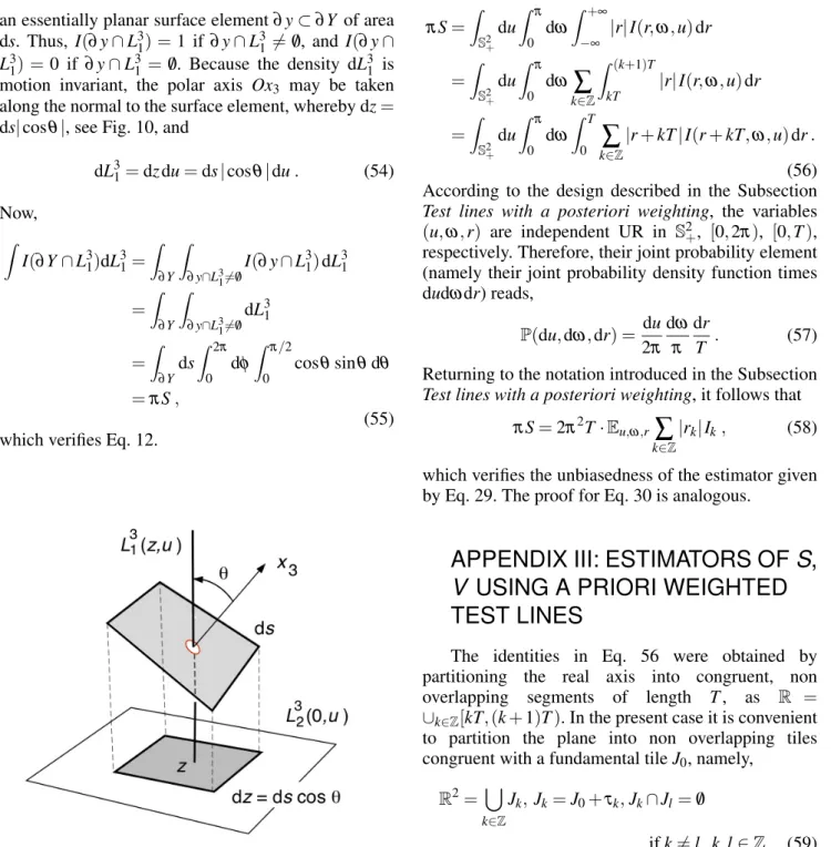
an essentially planar surface element∂y⊂∂Y of area ds. Thus, I(∂y∩L31) =1 if∂y∩L31 6= /0, and I(∂y∩ L31) = 0 if ∂y∩L31 = /0. Because the density dL31 is motion invariant, the polar axis Ox3 may be taken
along the normal to the surface element, whereby dz= ds|cosθ|, see Fig. 10, and
dL31=dzdu=ds|cosθ|du. (54)
Now,
Z
I(∂Y∩L31)dL31=
Z
∂Y
Z
∂y∩L316=/0
I(∂y∩L31)dL31
=
Z
∂Y
Z
∂y∩L316=/0
dL31
=
Z
∂Y
ds
Z 2π
0
dφ Z π/2
0
cosθsinθdθ
=πS,
(55) which verifies Eq. 12.
Fig. 10. Geometric elements to obtain the motion invariant density of a straight line hitting a surface element.
APPENDIX II: ESTIMATORS OF
S
,
V
USING A POSTERIORI
WEIGHTED TEST LINES
Write I(r,ω,u) = I ∂Y∩L32(0,u)
∩L21(r,ω) , for short. Eq. 17 may be expressed as follows,
πS= Z
S2+ du
Z π
0
dω Z +∞
−∞
|r|I(r,ω,u)dr
=
Z
S2+ du
Z π
0
dω
∑
k∈Z
Z (k+1)T
kT
|r|I(r,ω,u)dr
=
Z
S2+ du
Z π
0
dω Z T
0 k
∑
∈Z
|r+kT|I(r+kT,ω,u)dr.
(56) According to the design described in the Subsection Test lines with a posteriori weighting, the variables (u,ω,r) are independent UR in S2+, [0,2π), [0,T),
respectively. Therefore, their joint probability element (namely their joint probability density function times dudωdr) reads,
P(du,dω,dr) = du 2π
dω
π dr
T . (57) Returning to the notation introduced in the Subsection Test lines with a posteriori weighting, it follows that
πS=2π2T·Eu,ω,r
∑
k∈Z|rk|Ik, (58)
which verifies the unbiasedness of the estimator given by Eq. 29. The proof for Eq. 30 is analogous.
APPENDIX III: ESTIMATORS OF
S
,
V
USING A PRIORI WEIGHTED
TEST LINES
The identities in Eq. 56 were obtained by partitioning the real axis into congruent, non overlapping segments of length T, as R = ∪k∈Z[kT,(k+1)T). In the present case it is convenient
to partition the plane into non overlapping tiles congruent with a fundamental tileJ0, namely,
R2= [
k∈Z
Jk,Jk=J0+τk,Jk∩Jl =/0
ifk6=l,k,l∈Z. (59)
Every tile Jk can be brought to coincide with the
fundamental tile J0 by means of a translation −τk
which leaves the partition unchanged. Here J0 ⊂
L32(0,u) is adopted to be a square of area a. Write I(z,u) =I
n
∂Y∩L23(0,u)∩L21[·](z)
o
, for short. Now Eq. 24 may be written as follows,
πS= Z
S2+ du
Z
R2
I(z,u)dz
=
Z
S2+ du
∑
k∈Z
Z
Jk
I(z,u)dz
=
Z
S2+ du
Z
J0k
∑
∈Z
I(z+τk,u)dz.
The variables(u,z)are independent UR inS2+,J0,
respectively, so that,
P(du,dz) = du 2π
dz
a . (61)
Returning to the notation introduced in the Subsection Test lines with a priori weighting,
πS=2πa·Eu,z(I), (62)
which verifies the unbiasedness of the estimator given by Eq. 34. The proof for Eq. 35 is analogous.
The technique used in this, and in the preceding subsection, is a direct application of a theorem given in Ch.8 of Santal´o (1976); see also Cruz-Orive (2002), (Eq. 4.6).
APPENDIX IV: THE INTEGRATED
NUCLEATOR, AND THE PIVOTAL
NUCLEATOR, AS DIRECT
CONSE-QUENCES OF THE INVARIATOR
EQUATION FOR VOLUME
Write L(r,ω,u) = L Y∩L32(0,u)∩L21(r,ω) , for short. Eq. 18 may be written as follows,
2πV = Z
S2+ du
Z π
0
dω Z +∞
−∞
|r|L(r,ω,u)dr. (63)
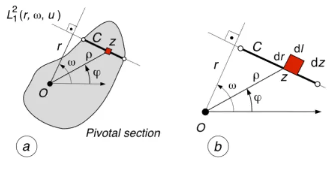
The length of the chord Y∩L32(0,u)∩L21(r,ω)≡C, say, (Fig. 11a), may be expressed as the integral of a length element dlalong the extent ofC, so that,
Z +∞
−∞
|r|L(r,ω,u)dr= Z +∞
−∞
|r|dr
Z
C
dl. (64)
The length elements dr and dl are orthogonal, and therefore drdl=dz is the area element at a point of the pivotal section, namely of z ∈Y ∩L32(0,u), see Fig. 11b. Let(ρ,ϕ)denote the polar coordinates of the pointz. Then|r|=ρ|cos(ω−ϕ)|, whereby,
2πV = Z
S2+ du
Z π
0 dω Z
Y∩L32(0,u)ρ
|cos(ω−ϕ)|dz
=
Z
S2+ du
Z
Y∩L32(0,u)ρ(z,u)dz Z π
0
|cos(ω−ϕ)|dω
=2
Z
S2+ du
Z
Y∩L32(0,u)
ρ(z,u)dz,
(65) which is the identity Eq. 36.
Fig. 11.Geometric elements involved in Appendix IV, see text.
The verification of the unbiasedness of the discretized nucleator Eq. 41 is immediate using Santalo’s theorem as in the preceding appendix.
To obtain the pivotal nucleator identity (40) for a star convex set with respect to O, replace dz with its polar coordinate version dz =ρdρdω in the last Eq. 65, whereby,
2πV =2 Z
S2+ du
Z 2π
0
dϕ
Z l+(ϕ,u)
0
ρ2dρ
=2 3
Z
S2+ du
Z 2π
0
l+3(ϕ,u)dϕ.
(66)
APPENDIX V: EQUIVALENCE
BETWEEN THE DIRECT AND
THE PIVOTAL NUCLEATOR
REPRESENTATIONS
Let(ρ,u),ρ≥0,u∈S2denote the spherical polar coordinates of a point x ∈ R3. The corresponding volume element is dx=ρ2dρdu. The volume of a star convex setY with respect to an interior originO∈Y may then be expressed as follows,
V =2
Z
S2 du
Z l+(u)
0
ρ2dρ
=1 3
Z
S2
l+3(u)du,
(67)