CONSIDERATIONS ON A POSTERIORI PROBABILITY
Corrado Gini (1911)
This paper is the “First part” of an assay published in the “Studi Economico-Giuridici della Universit di Cagliari”, year III, 1911. It was reprinted in “Metron” vol. XV, 1-4,1949.
1. To determine the probability that a phenomenon A takes place xtimes in s
future observations, is a problem that frequently occurs and the importance of which is such that it would be unnecessary to emphasize it.
Most of the time we are not in a position to solve it on the basis ofa priori
notions of the probability ofAtaking place. Notions of this type are found in the games that human beings have conventionally set up, provided that the instru-ments used do not show detectable irregularity in their makeup. But usually, to assess the probability of phenomenonA taking place insfuture observations, we must base our reasoning on its frequency in the previousnobservations, by resort-ing to the hypothesis that the probability of its takresort-ing place is constant durresort-ing the
n+sobservations. In such a case, we proceed to thea posteriori determination of the probability.
The problem of a posteriori determining the probability of future events, in its more general form, can be formulated as follows: Determine the probability that the phenomenon A occurs x times in s future observations, knowing that in Aprevious observations it did occur in times and supposing that, during then+s observations, its probability to occur remains unchanged.
2. In this study, we shall generally define Pb,c, the probability1 that the
phe-nomenonAtakes placebtimes incobservations; specificallyP1,1, more brieflyP,
will denote the probability of the occurrence ofA, withd,ePb,c let us denote the
probability thatAtakes placebtimes incobservations, when it has taken placed
times ineobservations. Hence, the probability thatAoccurs xtimes insfuture observations, when it has occurredmtimes inApast observations, will bem,nPx,s;
in particularm,nP1,1, that is more brieflym.nP, will denote the probability of the
occurrence ofA when it has occurred mtimes in nprevious observations. m,nP
1
is usually called thea posteriori probability of A.
3. To say that the probability of occurrence ofAremains unchanged duringn+s
observations, is equivalent to saying that what remains unchanged is the ratio of favorable events ofA occurring to the unfavorable events. We will than say that phenomenon A is dependent on A same system of causes, during the course of
n+sobservations2.
Now we can present two situations: either phenomenonAallows only one sys-tem of causes; or it allows several. For example, sunrise, from the beginning till the end of the world, is the consequence of A unique system of causes; the pro-portion of wins of A competitor (cyclist, racing driver, fencer or target shooter) over another, in one-day competitive games, permits instead as many systems of causes, as are the possible combinations of strength, with which, in one day, the two competitors may find themselves faced with. But, the first can be looked at as the limiting case of the second, which occurs when, among the various systems of causes on whichAmay depend, one has a probability equal to 1 and the others a probability equal to 0. One can therefore consider the second case only as the general one.
4. Letν be the systems of causes compatible with phenomenon A. Let us denote withm,nry the probability that, whenAhas occurredmtimes innobservations,
the system of causes ythis in action and, with yPx,s the probability that, if it is
acting, phenomenonAtakes place xtimes in sobservations. It will be
m,nPx,s= ν ∑
y=1
m,nry · yPx,s (1)
If py is the probability that generally the system of causes yth takes place
and yP
m,n is the probability that, if it is acting, A takes place m times in n
observations, it will be (for the well known Bayes theorem):
m,nry=
py yPm,n ν
∑
y=1
py yPm,n
(2)
2
hence
m,nPx,s= ν ∑
y=1
py yPm,nyPx,s
ν ∑
y=1
py yPm,n
(3)
The practical importance of this result is at any rate almost nil. The value of yPm,n and yPx,s could easily be determined if the probabilityyP was known,
thatA occurs when the system of causesythis in action. But (except for certain conventionally arranged games) we lack in this case the knowledge ofyP, as well
as that ofpy, becoming thus impossible to determine the value ofm,nPx,s, on the
base of (3).
Due to this ignorance, some believe they can resort to the hypotheses thatν
is infinitely large, that py is equal for all the ν systems of causes and that yP
assumes, asy varies, all the infinite values between 0 and 1. In suchAcase it is demonstrated3that it is
m,nPx,s=
s!(m+x)!(n−m+s−x)!(n+ 1)!
x!(s−x)!(s+n+ 1)!m!(n−m)! (4)
and in particular
m,nP = m+ 1
n+ 2 (5)
But, it is evident that these hypotheses are totally arbitrary. It is true that some authors have stated that, ifnis very large, one might assume to use formula (5), even when these hypotheses are not satisfied4, but there is no valid proof of such a statement and we will later note (§9) how, generally, this is not correct.
5. The determination of a posteriori probability, according to the outline con-sidered in the previous paragraph, presumes somea prioriinformation, regarding the number and the probability of the different systems of causes and regarding the probability that when each of them takes place, phenomenonA occurs. We may say that this is ana priori outline for the a posteriori determination of prob-ability. We shall call it: method for thea posteriori probability determination of
Aphenomenon on the base of the probability of causes.
I believe that to this, one can conveniently counterpoise an a posteriori way for the a posteriori determination of probability.
Instead of starting from the consideration of the various systems of causes, which might affect the occurrence ofAinn+sobservations, when it has occurred
mtimes innobservations, we start from the consideration of the various timesA
can occur inn+sobservations, when it has occurred mtimes innobservations.
3
See, for the proof, E. Czuber,Warhrscheinlichkeitsrechnung. 1. H¨alfte Leipzig, Teub-ner, 1902, p. 165.
Each one of these numbers represents adirect result.
WhenAhas taken placemtimes in nobservations, in then+sobservations it can occurm, m+ 1, m+ 2, . . . , m+stimes. Therefore there ares+ 1 possible
direct results.
We shall callithdirect result the one according to which the phenomenon A
occursm+itimes inn+sobservations.
We shall call this scheme: method for the a posteriori determination of the probability of phenomenon based on the probability of direct results.
m+1,n+sPi,sdenotes the probability that, when one obtains theithdirect result,
that is when A has occurred m+ 1 times inn+s observations, A has occurred
m times in the first n observations, i.e. i times in the lasts observations. This holds, in the hypothesis that the probability ofAoccurring keeps constant during then+sobservations.
Withfi=Pm+1,n+s we denote the probability that theithresult occurs, with Pm,n, the probability that phenomenonAoccursmtimes in nobservations.
The probability that A occurs m times in n observations and i times in the following s observations will be, by the theorem of conditional probability,
Pm,n m,nPi,s.
The probability thatAoccurs tom+itimes inn+sobservations anditimes in the lastsobservations will be, by the same theorem,fi m+i,n+sPi,s.
On the other hand, to say that phenomenonAoccursmtimes innobservations and itimes in the following sobservations, amounts to say that A occursm+i
times in then+sobservations and itimes in the lastsobservations. Hence we can write:
fi m+i,n+sPi,s=Pm,n m,nPi,s
from which
m,nPi,s=
fi m+i,n+sPi,s Pm,n
It follows that
m,nPx,s s ∑
i=0
m,nPi,s
= fsx m+x,n+sPx,s
∑
i=0
fi m+i,n+sPi,s
and, as it is∑si=0 m,nPi,s= 1
m,nPx,s=
fx m+x,n+sPx,s s
∑
i=0
fi m+i,n+sPi,s
(6)
When the probabilityP of the phenomenonA occurring remains constant in then+sobservations, the value ofm+i,n+sPi,s, is given by the formula5
5
m+i,n+sPi,s=
s!(m+i)!(n+s−m−i)!n!
i!(s−i)!(n+s)!m!(n−m)! (7) Then (6) becomes
m,nPx,s= fx
(m+x)!(n+s−m−x)!
x!(s−x)!
s ∑
i=0
fi
(m+i)!(n+s−m−i)!
i!(s−i)!
(8)
In the particular cases= 1,x= 1, it is
m,n+1P0,1=
n−m+ 1
n+ 1 m+1,n+1P1,1=
m+ 1
n+ 1 hence
m,nP =
R(m+ 1)
R(m+ 1) +n−m+ 1 (9)
whereR=f1 f0
Often statistical surveys allow to determine, fromA large enough number of observations, the frequencies with which the various direct results occur. Such frequencies can be thought of, as approximate values of the related probabilities
fi.
Then it becomes easy to calculate the value ofm,nPx,s.
Let us give some examples.
6. Example 1. We are dealing with A trigeminous birth. The woman con-cerned has already given birth to 2 males. The third baby is expected. What is the probability that it will also be a male?
There are 2 possible direct results: 3 males; 2 males and 1 female.
frequency with which it has taken place in the previousnobservations. It is then
Pm,n m,nPi,s=Pm,nPi,s
And remembering that it isfi=Pm+1,n+s
Pm+i,n+s m+i,n+sPi,s=Pm,nPi,s
m+i,n+sPi,s=
Pm,nPi,s
Pm+i,n+s
By substituting, in this equation, forPm,n, Pi,s, Pm+i,n+sthe values given by the known
formula
Pb,c=
c!
b!(c−b)!P
b
(1−P)c−b
Statistics points out that in 100 trigeminous births, in 24 cases all 3 were males and in 27 cases there were 2 males and 1 female (Italy: 1884-95).
When the direct result obtained is: 3 males, the probability that the first two born were males is equal to 1.
When the direct result obtained is: 2 males and 1 female, the probability that the first two born are males is 1/3, on the hypothesis that the probability of a male birth does not vary with the generation order.
The theoretical probability that the third born in a trigeminous birth is a male, when the first two were males, will be
24×1
24×1 + 27×1/3 = 24 33 that is, approximately, 3/4.
From here onwards, I use the expression “theoretical probability” to define the probability m,nPx,s calculated on the hypothesis that probability P remains
constant for then+sobservations.
Example 2. A two-race match is run between A and B. CompetitorA has already won one race. What is the probability that he will win the second as well? The race bulletin allows us to establish that, in the course of the numerous encounters betweenA and B, A won both races 35 out of the 100 times, 50 out of the 100 he won one race only, and 15 out of the 100 he lost both races.
In our case, only two direct results are possible: either A wins both of the races, or he wins only one. IfAwins both the races, there is a probability equal to 1 that he has won the first race. IfAwins one race out of two, and the probability of winning is independent of the order of the races, there is a probability equal to 1/2 that he has won the first race.
The theoretical probability that he wins the second race, when he has won the first, will therefore be
35 35×50/2 =
7 12.
Example 3. A couple has up to now given birth to 3 males and 1 female: what is the probability that they will have, in the next two deliveries: 2 males; 1 male 1 female; 2 females?
There are 3 possible direct results: 5 males and 1 female; 4 males and 2 females; 3 males and 3 females.
Statistics shows that the frequencies of these three direct results are related to each other almost at the ratio 10:23:30 (Saxony 1876-85).
If the probability of having a male or a female is constant during the entire fertile period, the probability of having had, in the first 4 births, 3 males and 1 female is easily found by (7), to be 2/3 for those who, in 6 births, had 5 males and 1 female, 8/15 for those who, in 6 births, had 4 males and 2 females, 1/5 for those who, in 6 births, had 3 males and 3 females.
The couple that has so far given birth to 3 males and 1 female then has the theoretical probability
23×8/15
of giving birth in the next two deliveries to one male and one female. The couple has the theoretical probability 50/187 of giving birth to 2 males, and the theoretical probability 45/187 of giving birth to 2 females.
Example 4. Let us consider a similar case. Until now a couple had 2 males and 4 females. They lost the 2 males and would like to have another one: what is the probability of their having another child of male sex?
There are two possible direct results: 3 males and 4 females, 2 males and 5 females.
Let us assume that statistics tells us only that the frequency of the first direct result is to that of the second as 191 is to 107 (Saxony: 1876-85).
If the probability of having a male is constant during the entire fertile period, the probability of having 2 males and 4 females in the first 6 births is 3/7 when, in 7 births, we have 3 males and 4 females and 5/7 when in 7 births, we have 2 males and 5 females.
The theoretical probability that the said couple will have a male child in the 7thbirth is then
191×3/7
191×3/7 + 107×5/7×1/5 = 0.517.
7. In the previous examples we have always talked about theoretical probabil-ities. One would expect that these probabilities would not differ systematically from the actual frequencies, if the hypothesis from which we started was correct: the probability of the considered phenomenon occurring remains constant dur-ing the n+s observations. Sometimes the statistical data enable us to directly calculate the actual frequencies and the comparison between the latter and the theoretical probabilities allows to verify if the probability of A occurring keeps truly constant during then+sobservations or if it instead varies, and how.
For example, statistics enable us to establish that in Saxony (1876-85), 15,700 couples, who had 2 males and 4 females, had a 7thmale in 53% of the cases. The
theoretical probability was instead less than 52%. (§6, example 4). This differ-ence introduces the doubt that the probability of having a male does not remain constant during the entire fertile period. The subject is far too interesting not to bother to go deeper into it. The second part of the study deals with it.
8. Let us consider the particular case in which all the “direct results” have the same probability. In such a case it will be
m,nPx,s=
m+x,n+sPx,s s
∑
i=0
m+i,n+sPi,s
(10)
the value given by the following formula6:
s ∑
i=0
m+i,n+sPi,s=
n+s+ 1
n+ 1
we obtain
m,nPx,s=
s!(m+x)!(n−m+s−x)!(n+ 1)!
x!(s−x)!(s+n+ 1)!m!(n−m)! (11) This formula is identical to (4).
The probability that the phenomenon takes place x times in s observations, when it has occurredmtimes innprevious observations is therefore the same: a) when thes+ 1 direct results are equally probable;b) when the phenomenon allows with the same probability an infinite number of systems of causes, according to which the phenomenon has a probability of occurrence which ranges from 0 to 1.
Ifs= 1,x= 1, (11) becomes7
m,nP = m+ 1
n+ 2 (12)
that gives thea posteriori probability of phenomenonA, when it has occurredm
times innprevious observations. (12) is identical to (5).
Thea posteriori probability of phenomenonA, that has occurredm times in
nprevious observations, is therefore the same: α) when, inn+ 1 observations,A
has the same probability of occurringmorm+ 1 times;β) when the phenomenon allows, with the same probability, an infinite number of systems of causes, accord-ing to which the phenomenon has a probability of occurraccord-ing which ranges from 0 to 1.
It is obvious that, having satisfied condition α), condition β) may not be satisfied. It may in fact be that phenomenon A has the same probability of occurringmorm+ 1 timesn+ 1 observations and that it does not allow certain systems of causes. For example, a phenomenon may have the same probability of occurring 24 and 26 times in 50 observations and allow only 2 systems of causes, according to which it has a probability of occurring of 24/50 and 26/50 respectively. It can instead be demonstrated that, if conditionβ) is fulfilled, conditionα) is as well.
IfyP is the probability of phenomenonAoccurring when the system of causes yth is in action, the probability that A takes place in m+ 1 times on n+ 1
observations, will be
yP
m+1,n+1=
(n+ 1)! (m+ 1)!(n−m)!
yPm+1(1−yP)n−m
6
The proof of this equation is attributed to Prof. Luigi Galvani, Assistant Professor of Differential calculus in the R. University of Cagliari. It is shown in the Appendix to [the original] paper.
7
This formula can be directly deduced from (9), noting that in such a case it isf1=f0,
If there are infinite systems of causes, all equally probable, according to which
yP assumes the infinite values from 0 to 1, the probability p
y that system yth
becomes active will be constant and it will be possible to set it equal to the differencedyP between 2 successive values ofyP.
Hence, the probability thatAoccursm+ 1 times inn+ 1 observations will be
Pm+1,n+1=
(n+ 1)! (m+ 1)!(n−m)!
∫ 1
0
yPm+1(1−yP)n−m dyP (13)
By partial integrations, it is found that
∫ 1
0
xh(1−x)kdx= h!k! (h+k+ 1)! hence
Pm+1,n+1= 1
n+ 2 Likewise it is demonstrated that
Pm,n+1=
(n+ 1)!
m!(n−m+ 1)!
∫ 1
0
yPm(1−yP)n−m+1dyP = 1
n+ 2 (14) hence
Pm,n+1=Pm+1,n+1 Conditionα) is then weaker thanβ).
Thus, by means of formula (5), we have found a validity condition which is more general than the one which is commonly proposed, that the phenomenon allows, with equal probability, infinite systems of causes, according to which its probability of occurring may take any of the infinite values from 0 to 1.
It is true that some authors maintain that, as stated earlier, whenn is very large, the formula (5) remains valid even when the various systems of causes do not have the same probability of acting; but how this is not generally true will be demonstrated in the following paragraph.
9. Let us consider a more general situation than that examined in the previous paragraph.
Let us again assume that there are infinite systems of causes, according to whichyP assumes the infinite values from 0 to 1; the probability that the system
of causesythoccurs, is
Py=
(k+h+ 1)!
k!h!
yPk(1−yP)h dyP (15)
where the constantk andhare integer positive numbers8.
8
In the particular case whenk= 0, h= 0 it ispy =d yP and one goes back to the
It is
ν ∑
y=1
Py = 1.
Instead of (13), it is then
Pm+1,n+1=
(n+ 1)! (m+ 1)!(n−m)!
(k+h+ 1)!
k!h!
∫ 1
0
yPm+k+1(1−yP)n−m+hdyP
and instead of (14),
Pm,n+1=
(n+ 1)!
m!(n−m+ 1)!
(k+h+ 1)!
k!h!
∫ 1
0
yPm+k(1−yP)n−m+h+1dyP
From which
R=Pm+1,n+1
Pm,n+1
= m+k+ 1
m+ 1
n−m+ 1
n−m+h+ 1
and, on the basis of (9),
m,nP =
m+k+ 1
n+k+h+ 2 (16)
Becausekandhmay assume any integer positive value, it is obvious that the value of formula (16), for any n, may differ essentially from the value of formula (5).
10. To determine the probability that a phenomenon A, which has occurred
m times inn observations, will occur itimes in the following sobservations, we cannot always make use of the frequency with which phenomenonAoccursm+i
times in n+s observations. One often knows only the frequency with which phenomenonAoccurs m+y times inn+t observations, wheret > s.
WhenA takes place m+i times in n+s observations, we said that theyth
direct result occurs; whenAtakes placem+ytimes inn+ 1 observations, we will say that theythindirect result occurs.
Let us try to define ana posteriorischeme for thea posterioridetermination of the probability, a scheme more general than the one we considered in§5, which is based on the frequency of the results, irrespective of these being direct or indirect. In general, we will call it: scheme to a posteriori determine the probability of a phenomenon, on the basis of the probability of the results9.
9
Let us denote withfy the probability that theythresult occurs. Given all the
values offyit is easy to calculate the single values offion the basis of the formula
fi= i ∑
y=0
fy m+y,n+1Pm+1,n+s
Instead of (6), we must therefore put
m,nPx,s= t ∑
y=0
fy m+y,n+tPm+x,n+s m+x,n+sPx,s
s ∑ i=0 t ∑ y=0
fy m+y,n+tPm+i,n+s m+1,n+sPi,s
(17)
To calculate the second member of this equality it can be noted that, when the probability of the occurrenceA is constant in then+t observations, it is
m+y,n+tPm+i,n+s=
(t−s)! (y−i)!(t−s−y+ 1)!
(m+y)!(n+t−m−y)! (n+t)!
(n+s)!
(m+i)!(n+s−m−i)!
(18)
From (18) and from (7), one can easily deduces that the numerator of (17): it is
= t ∑ y=0 fy s!
x!(s−x)!
n!
m!(n−m)! (t−s)!
(y−x)!(t−s−y+x)!
(m+y)!(n+t−m−y)! (n+t)!
(19)
and the denominator
= t ∑ y=0 ( fy n!
m!(n−m)!
(m+y)!(n+t−m−y)! (n+t)!
s ∑
i=0
s!
i!(s−i)!
(t−s)! (y−i)!(t−s−y+i)!
) (20)
Note now that it is
s ∑
i=0
s!
i!(s−i)!
(t−s)! (y−i)!(t−s−y+i)!
y!(t−y)!
t! = 1
and hence
s ∑
i=0
s!
i!(s−i)!
(t−s)!
(y−i)!(t−s−y+i)! =
t!
Substituting this value in (20), dividing (19) by (20) and by simplification, one obtains
m,nPx,s=
s!(t−s)!
t!
t ∑
y=0
fy
(m+y)!(n+t−m−y)!
x!(s−x)!(y−x)!(t−s−y+x)!
t ∑
y=0
fy
(m+y)!(n+t−m−y)!
y!(t−y)!
(22)
In the particular caset=s, y=i, (22) is easily simplified to (8), remember-ing10 that it is 1! = 1, 0! = 1; (−K)! =∞.
11. Let us see which value (22) assumes, when fy is constant, that is when the t+ 1 results are equally probable. Because of this, let us observe that it is
t ∑
y=0
m+y,n+tPy,t=
n+t+ 1
n+ 1
from which it is immediately obtained
t ∑
y=0
(m+y)!(n+t−m−y)!
y!(t−y)! =
(n+t+ 1)!m!(n−m)!
(n+ 1)t! (23)
Likewise
t ∑
y=0
m+y,n+tPy−x,t−s=
n+t+ 1
n+s+ 1
from which it is easily obtained
t ∑
y=0
(m+y)!(n+t−m−y)!
x!(s−x)!(y−x)!(t−s−y+x)! =
(n+t+ 1)!(m+x)!(n+s−m−x)!
x!(s−x)!(n+s+ 1)!(t−s)!
(24)
Iffy is constant, and the values obtained from (23) and (24) are substituted
in (22), this becomes the same as (11).
Then, when thet+ 1 results (direct or indirect) are equally probable, the value ofm,nPx,sis independent oft; in other words, it is the same, whatever the number
of future observations to which the results are referred.
12. Let us apply (22) to an example.
10
From the combination concept it is immediately derived h(h!(−−KK)!)! = 0 from which
1
The first born in a trigeminous birth was a male: we want to find out the probability that the second born will also be a male.
There are three possible indirect results: 3 males, 2 males and 1 female; 2 females and 1 male; the respective frequencies of which are: f2= 24%;f1= 27%;
f0= 26%. (Italy, 1884-85).
On the basis of (22), the probability we are looking for is equal to 89/152, approximately 2/3.
This calculation presumes that the probability of having a male or a female is the same for the first, second or third child born in a trigeminous birth.
13. The a posteriori determination of the probability of A, on the basis of the probability of the “direct results”, assumes that the probability ofAremains con-stant in thenobservations already taken and in thesobservations yet to be taken. Thea posteriori determination of the probability of Aon the basis of the proba-bility of the indirect results assumes that the probaproba-bility of the occurrence ofA
remains constant in the nobservation already taken and in a numbert of future observations, which is greater than the numbersof observations yet to be taken. The hypothesis that the probability ofA remains constant for a given num-ber of observations will evidently be more plausible, the smaller the numnum-ber of observations considered.
This does not necessarily mean that the a posteriori determination of the probability ofA occurringi times insfuture observations is less precise when it is obtained on the basis of the probability of “indirect results”, than when it is obtained on the basis of the probability of the “direct results”. Nor that, when it is obtained on the basis of “indirect results”, it is much less precise, the greater is the numbertof future observations, to which the results are related. This con-clusion would be true when the probability of Adoes not vary in the first future observations and does vary in the subsequent observations, and likewise when it would vary continuously throughout all future observations, always increasing or always decreasing. But if, during future observations, it changes first in one direc-tion and then in the opposite one, it might be that thea posteriori determination of the probability is more precise when obtained on the basis of “indirect results”, than when it is based on “direct results”. It might also be that, when based on “indirect results”, it is more precise when the number of observations, to which the “indirect results” are related, is greater.
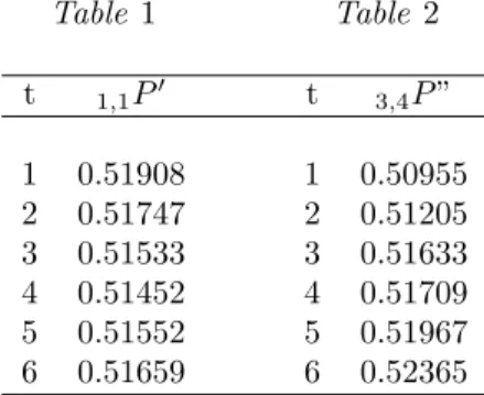
Let us verify this for the data on the sex of the newly born in Saxony (1876-85). The frequency with which a male is born in the second birth, when in the first
Amale was born, is1,1P” = 0,51931.
The theoretical probability1,1P′, calculated on the basis of the frequency of the result related totfuture observations, varies withtas follows [see Table 1].
Table 1 Table 2
t 1,1P′ t 3,4P”
1 0.51908 1 0.50955
2 0.51747 2 0.51205
3 0.51533 3 0.51633
4 0.51452 4 0.51709
5 0.51552 5 0.51967
6 0.51659 6 0.52365
in the first birth or in the first two births, the actual frequency of having a male in the following delivery is greater than the theoretical one; instead, the families which had all males in more than two births, in the next one show a frequency of having males which is less than the theoretical probability.
Instead, when in the past births the males are in excess, but there are some females as well, the actual frequency of having males in the following births is always less than the theoretical probability. Hence, it appears that the frequency of a male birth, after having hadm males and n−m < m females, differs from the theoretical probability determined on the basis of the frequency of the results inn+tobservations, and it differs more whentis greater. As an example, let us consider a family which, until now, had 3 males and 1 female. The frequency of having a male in the 5th birth is 3,4P” = 0.50350. The theoretical probability is as follows [see Table 2].
The difference between3,4P” and3,4P′ is very small for t= 1, increases with
tand becomes quite considerable fort= 6.
14. Formula (17) can be written in a different form. It must be noted that when the probability ofAremains constant in the n+tobservations, it is
m+y,n+tPm,n=
n!
m!(n−m−)!
(m+y)!(n+t−m+y)! (n+t)!
t!
t!(t−y)!
y,tpi,s = s!
i!(s−i)!
y!(t−y)!
t!
(t−s)! (y−i)!(t−s−y+i)!
From these formulae and from (19), (20), (21) it is
t ∑
y=0
fy m+y,n+tPm,n y,tPx,s= t ∑
y=0
fy m+y,n+tPm+x,n+s m+x,n+sPx,s
t ∑
y=0
fy m+y,n+tPm,n y,tPx,s= s ∑
i=0
t ∑
y=0
Hence, (17) can also be written as follows:
m,nPx,s= t ∑
y=0
fy m+y,n+tPm,n y,tPx,s
t ∑
y=0
fy m+y,n+tPm,n
(25)
15. Formula (25) is useful to show the relationship existing between the scheme for thea posteriori determination of the probability of a phenomenonA, on the basis of the probability of causes, and the scheme for thea posteriori determination of the probabilityA, on the basis of the probability of results.
Let us consider a specific case in whichtis infinitely large,xandmare negli-gible compared toy, andsandnare negligible compared tot.
As the probability is the limit to which the frequency of a phenomenon tends, as the number of observations increases, we could say that, whentis infinitely large, to different results correspond different probabilities of phenomenonAoccurring, i.e. different systems of causes. The first system of causes will correspond to result 0; the second system of causes to result 1; generally, the system of causes (y+ 1)th
will correspond to resultyth. We could that put
py+1=fy
and (see note (5))
m+y,n+tPm,n= y+1P
m,ny+1Py,t y+1P
m+y,n+t
y,tPx,s= y+1P
x,s x+1Py−x,t−s y+1P
y,t
But, asm andn are negligible compared toy and tot respectively, we could put
y+1P
y,t y+1P
m+y,n+t
= 1
hence
m+y,n+tPm,n=y+1Pm,n
Similarly, asxandsare negligible compared toy andtrespectively, we could put
y+1P
y−x,t−s y+1P
y,t
hence
y,tPx,s= y+1Px,s
If in (25)fy,
m+y,n+tPm,n andy,tPx,s are substituted by,py+1, y+1Pm,n and y+1P
The scheme for thea posteriori determination of the probability ofA, on the basis of the probability of causes may therefore be looked at as a particular case of the scheme of thea posteriori determination of the probability ofA, on the basis of the probability of the results; a situation which occurs when the probability determination is based on the probability of the “indirect results” from a very large number of observations.
16. By introducing a slight modification in (3), one obtains a formula for the
a posteriori determination of probabilities which is valid either for the method of the probability of results, or for the method of the probability of causes.
The occurrence of phenomenonAin thesfuture observations may depend on several systems of causes, or it may correspond to different “direct” or “indirect” results. Every system of causes, and similarly every result, may therefore be looked upon as an eventuality11.
We will indicate byν the number of the eventuality, bypythe probability that
theytheventuality will occur, byyP the probability of the occurring ofA,
accord-ing to the yth eventuality, by yP
x,s the probability that, in the yth eventuality, A will occur xtimes ins future observations, with y
m,nPx,s the probability that,
in theytheventuality, Awill occurxtimes ins future observations, when it has
occurredmtimes in npast observations.
Let us first suppose that the eventualities of which we know the single proba-bilitiespy consist in results. Adopting the new symbols, (25) becomes:
m,nPx,s= ν ∑
y=1
py yPm,nm,nyPx,s
ν ∑
y=1
py yPm,n
(26)
Let us now suppose that the evantualities, of which we know the single prob-abilitiespy consist insystem of causes. As the probabilityyP will be maintained
costant in n+sobservations, whatever the acting system of causes, it will be:
y
m,nPx,s=yPx,s
and so (3) may be written as (26).
Formula (26) can therefore he seen as the general formula to determine proba-bilitya posterioni. Confronted with it, (3) and (25) represent particular formulae, of very different usage, valid when the eventualities, on the basis of which probabil-ity isa posteriori determined, consist in systems of causes or results respectively.
11
Summary
In this first paper of 1911 relating to the sex ratio at birth, Gini repurposed a Laplaces succession rule according to a Bayesian version. The Gini’s intuition consisted in as-suming for prior probability a Beta type distribution and introducing the “method of results (direct and indirect)” for the determination of prior probabilities according to the statistical frequency obtained from statistical data.