Performance Limits Study of Stencil Codes on Modern
GPGPUs
Ilya S. Pershin1 , Vadim D. Levchenko2 , Anastasia Y. Perepelkina2
c
The Authors 2019. This paper is published with open access at SuperFrI.org
We study the performance limits of different algorithmic approaches to the implementation of a sample problem of wave equation solution with a cross stencil scheme. With this, we aim to find the highest limit of the achievable performance efficiency for stencil computing.
To estimate the limits, we use a quantitative Roofline model to make a thorough analysis of the performance bottlenecks and develop the model further to account for the latency of different levels of GPU memory. These estimates provide an incentive to use spatial and temporal blocking algorithms. Thus, we study stepwise, domain decomposition, and domain decomposition with halo algorithms in that order. The knowledge of the limit incites the motivation to optimize the implementation. This led to the analysis of the block synchronization methods in CUDA, which is also provided in the text. After all optimizations, we have achieved 90% of the peak performance, which amounts to more than 1 trillion cell updates per second on one consumer level GPU device.
Keywords: stencil computations, parallel algorithm, GPU, CUDA, Roofline model.
Introduction
The theoretical performance peak of the modern GPU exceeds 10 TFLOPS for single pre-cision, and this could be a trillion cell updates per second for a variety of stencil schemes. However, it is well known that this performance can not be achieved, since the stencil codes are not compute-bound [7]. The global memory throughput limit for modern GPU corresponds to approximately 1% of their peak computing performance. Furthermore, in the implementations of the stencil codes, other factors, such as data access overhead and latency, limit the performance. In this paper we study the performance limits of different algorithmic approaches, applied to a sample problem, and aim to find the highest limit of the achievable performance efficiency for the stencil computing. For this, we develop the implementation using the accumulated ex-perience of CUDA programming so as to minimize the performance losses. We use an advanced quantitative performance model to make a thorough analysis of the performance bottlenecks, and develop it further to account for the latency of different levels of GPU memory.
Increasing the performance efficiency of the stencil implementation is an intricate task, and multiple factors should be take into account. The cell update requires its data and the data from its neighbours to be accessed. Thus, each cell data is accessed multiple times during one time iteration, and the exact way this access is performed depends on the algorithm. The cache hierarchy is developed so as to accelerate the data accesses with high locality in time and space. To take advantage of it in the stencil computing, the tiling and blocking techniques are used [5, 8–10, 13, 14, 20, 27, 30]. These involve a modification of the data space traversal and decomposition of this task into subtasks that may be given to different processing units. Various polyhedral optimization techniques are based on this idea [6, 22].
Spatial tiling [5, 8–10, 13, 14, 20, 27, 30] involves only spatial directions and may be hierar-chical to incorporate different levels of cache.
Temporal tiling [5, 8, 13, 14, 20, 27, 30] is the method to perform several cell updates on the same data portion that is located in the fast memory. After this, more data will be sent,
1
Moscow Institute of Physics and Technology, Dolgoprudny, Russian Federation
2Keldysh Institute of Applied Mathematics RAS, Moscow, Russian Federation
although, there are less synchronization events. Hierarchical temporal tiling is a part of the Locally Recursive non-Locally Asynchronous (LRnLA) algorithms approach [25, 26].
The idea of the tiling applies to any system with hierarchical memory and levels of paral-lelism. It may be made cache-aware or cache-oblivious [12].
Concerning the stencil performance optimization on GPU, in the classical CUDA imple-mentation [32] the tiling is inherent and is obtained by tuning the CUDA kernel parameters so as the data of the tile fits shared memory. This foreshadowed the trend for 2.5D blocking 1D streaming algorithm [13, 24, 31], which may be used in conjunction with temporal blocking [20]. The best performance of the applied stencil codes reaches about 30% of the peak theoretical performance [17, 18, 29].
The algorithmic optimization is often not enough for the best performance, the programming tools should be used with care. This includes the knowledge of the compiler optimization trends and hardware specifics. This becomes the center point of some optimization strategies [11, 24] and promotes the development of stencil code generation frameworks [4, 23, 28].
Since the stencil computing is considered as a memory-bound problem, the performance limits and bottlenecks in most of the aforementioned works are studied from the consideration of the ratio of the cell updates that may be performed per data access operation and the memory throughput. This analysis has become more convenient with the introduction of the Roofline model [21]. We use it in this work, and propose the modification to form an image of the latency Roofline. In sum, this work combines the use of the most advanced algorithms, CUDA implementation techniques and performance analysis to provide a model for maximizing the performance of the stencil code implementation on GPU. For this purpose, we choose the finite-difference cross-stencil scheme for 1D wave equation.
The article is organized as follows. Section 1 serves to introduce the kind of numerical computation that is considered for the current work. In sections 2, 3, and 4 we discuss the three algorithmic approaches, namely, stepwise algorithm, recursive domain decomposition, and recursive domain decomposition with halo, correspondingly. In each section, we present the de-scription of the corresponding algorithm, details of its implementation, performance test results and the theoretical performance model in that order. At the end of sections 2 and 3, we evaluate the weak spots of each algorithm and propose the direction of further study. In the Conclusion, we summarize the achievements and propose the practical applications of the presented research.
1. Problem Statement and Cross Stencil
The following (2r+ 2)-point stencil computation is constructed (Fig. 1):
unk+1 =−unk−1+α0unk+α−1unk−1+α1unk+1+. . .+α−runk−r+αrunk+r
| {z }
(2r+1) terms
. (1)
Here r is the stencil radius (half-width), unk =u(xk, tn), {(xk, tn) = ((k+12)∆x, n∆t), k ∈ [0, K), n ∈ [0, N)}. The values of α±l for specific r may be readily computed manually or generated with scripts [19].
2. Stepwise Algorithm
Figure 1. Cross stencils forr= 1,2,3: 3 time layers, 2r+ 1 points in space on the middle layer; the blue dots are read and the green dot is updated in the stencil computation
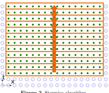
Figure 2. Stepwise algorithm
to implement with the tools available in CUDA [15]. However, even in this case care must be taken to get close to the optimal performance.
The two time layersunand un−1 are stored in the global memory. The computation kernel computes one update for each cell according to the stencil (1). Each thread is assigned to one cell [32]. In total,K/threadsCUDA-blocks are executed, wherethreadsis the number of threads per block (usually 1024 or512or256). This CUDA-kernel is executedN times in a CPU loop. The stepwise algorithm is illustrated in terms of the problem dependency graph in Fig. 2. One point represents one un
k computation. Inside the outlined areas there are no data dependencies. The domain size in x is limited by the size of the device memory, which means that about 109 cells may be stored. There is a data dependency between adjacent outlined areas, as shown by the arrow. After a CUDA-kernel computes one such area and exits, the data is synchronized, and the next loop iteration is started.
2.1. Performance Testing
The dependency of the performance of the stepwise kernel on the problem size has been tested. The number of cell updates per second (cell·sstep) is chosen as a unit for performanceP. Thus,P = Ktime·N where timeis the time per program run in seconds.
104 104 105 105 106 106 107 107 108 108
K, number of cells in the grid
100 100
101 101
102 102
P, pe rfo rm an ce , 1 0
9 of
[c
ell
ste
p/
s]
RTX 2070, radius = 1 RTX 2070, radius = 2 RTX 2070, radius = 3 GTX 1070, radius = 1 GTX 1070, radius = 2 GTX 1070, radius = 3
a) Single precision
104 104 105 105 106 106 107 107 108 108
K, number of cells in the grid
100 100
101 101
102 102
P, pe rfo rm an ce , 1 0
9 of
[c
ell
ste
p/
s]
RTX 2070, radius = 1 RTX 2070, radius = 2 RTX 2070, radius = 3 GTX 1070, radius = 1 GTX 1070, radius = 2 GTX 1070, radius = 3
b) Double precision
Figure 3. The stepwise algorithm performance dependence on problem size
At the start the linear increase is observed, due to low occupancy [1] of high parallel GPU device. The number of threads that may be started on an Streaming Multiprocessor (SM) de-pends on the required registers number (up to 64 thousand 32 bit registers per SM) and the shared memory size per thread (up to 48–64KB). The stepwise kernel does not use the shared memory explicitly and uses no more than 32 registers per thread. Thus, each SM may process up to 2048 cells simultaneously. There are 15 SM on GTX 1070 and 36 SM on RTX 2070. Therefore, 30 thousand and 72 thousand cells are required to utilize all resources of GTX1070 and RTX2070 correspondingly. This is in accordance with the cell number K value at which the performance P stops the linear increase. It gradually saturates, then falls to the constant P =Psw ∼1010 cell·sstep.
We note that in the single-precision computation the performance does not depend on the stencil radius. This is an evidence that the current implementation is memory-bound, since the operation count increases with the stencil radius. For double precision a slight variation in performance for different r is observed. In that case, the problem is closer to compute-bound domain since the peak computing performance for double precision is much lower.
The peak at K = 105 is clearly seen in the single-precision performance, which is higher than Psw. It is explained by the use of the L2 cache. Since the problem is memory-bound,P is determined by the global memory bandwidth. When the data may be localized in the L2 cache (2MB for GTX 1070, 4MB for RTX 2070), L2 memory bandwidth determines the performance. It is 1.5-2 times higher. This size corresponds to K = 2.5·105 and K= 5·105 cells with single precision, which is exactly the location of the end of the peak and transition toPsw.
2.2. Roofline Model
The Roofline [21] is a visual performance model that provides an estimate of the performance limit from the two fundamental ceilings: peak computing performance and memory bandwidth:
Πalg≤min(Πpeak,Θ·Ialg). (2)
Ialg = DOalgalg is the arithmetic intensity of the algorithm, whereOalg is the number of operations in the algorithm and Dalg is the data traffic to and from memory.
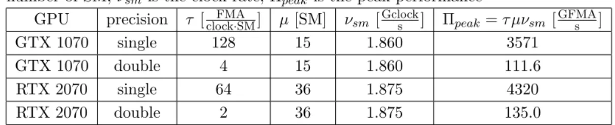
Usually, Πpeak and Θ are taken from the device specification. However, since these values depend on the frequency which may vary in wide range, they should be calculated accurately as follows. Arithmetic instruction throughputτ is the number of instructions that may be executed per cycle. These values can be found in [3], and are determined by the GPU architecture. The number of SM µ can be obtained by CUDA Runtime API. To get the actual frequency of SM νSM, the monitoring tools (such asnvidia-smi ornvidia-settings) are run during the code execution, since the frequency may depend on many factors. Then, Πpeak =τ µνSM. Similarly, with the use of CUDA Runtime API the memory bus width β can be found out. With the use of monitoring tools the memory frequency νmem is measured during the code run. Thus, Θ = 2βνmem. The factor of 2 is explained by the Graphics Double Data Rate SDRAM (GDDR SDRAM) feature. All these values are collected in Tab. 1 and Tab. 2.
Table 1. GPU characteristics: τ is the arithmetic instruction throughput, µ is the
number of SM,νsm is the clock rate, Πpeak is the peak performance
GPU precision τ [clockFMA·SM] µ [SM] νsm [Gclocks ] Πpeak=τ µνsm [GFMAs ]
GTX 1070 single 128 15 1.860 3571
GTX 1070 double 4 15 1.860 111.6
RTX 2070 single 64 36 1.875 4320
RTX 2070 double 2 36 1.875 135.0
Table 2. GPU characteristics: β is the memory bus width,
νmem is the memory clock rate, Θ is the memory bandwidth GPU β [clockB ] νmem [Gclocks ] Θ = 2βνmem [GBs ]
GTX 1070 32 3.802 243.3
RTX 2070 32 6.801 435.3
The unit for measurement of the performance Π is one Fused Multiply Add (FMA) operation, which may be one or two floating point operations (FLOP), while the symbol P is used for performance in cell updates. The compiler might optimize all operations to FMA. However, we have decided to force compiler to use FMA operations whenever possible via intrinsic (built-in) functions.
For one cell update Oalg = (2r + 1) cellFMA·step operations are required. The operations are grouped manually into FMA as follows:
unk+1 =α±r(
FMA
z }| {
unk+r+unk−r) +. . .+α±1(
FMA
z }| {
unk+1+unk−1) +
FMA
z }| {
α0unk−un −1 k
| {z }
FMA
| {z }
FMA
.
the required number of the L2 accesses it is necessary to take into account the possibility of misaligned access to the cache lines of the neighbor cells. The number of accesses to L1 about twice more that the number of accesses to L2, and it is much faster than the global memory. Thus, the L1 exchange may be neglected in the Roofline model. Data throughput is Dalg = 12 cellB·step for single precision and Dalg= 24 cellB·step for double precision. The arithmetic intensity is
Ialg= Oalg Dalg = 2r+1
12 FMA
B , for single precision 2r+1
24 FMA
B , for double precision
. (3)
The performance Πalg [GFMAs ] is computed from the performance Psw[cell·sstep], that was obtained as a saturated performance for large K in the performance tests, andOalg [cellFMA·step] as
Πalg =Psw·Oalg. (4)
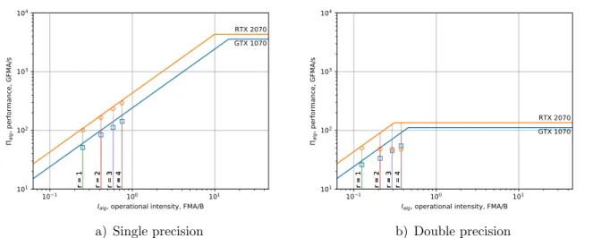
The Roofline graph for our implementation of the stepwise algorithm with data localization in the global memory is plotted in Fig. 4.
For single precision, our results fall into the memory-bound domain. The performance is limited by the global memory bandwidth. The overhead is observed to be negligible, as the result is close to the ceiling. With the increase of the stencil radiusr the performance increases, due to the increase in the arithmetic intensity. However, peak performance to memory bandwidth ratio is about 100 times more then optimal ratio for stencil calculations with stepwise algorithm. The double-precision peak performance on the chosen GPU is 32 times lower than single-precision peak ones, so performance to memory bandwidth ratio is closer to operation intensity. At r= 1 the result falls into the memory-bound area, and as the arithmetic intensity increases, the result comes closer to the compute-bound domain, and reaches it atr = 4. The performance is 40–50% of Πpeak and does not increase in the compute-bound domain.
It is likely that if a Tesla architecture GPU is used, the Roofline would look similar for single and double precision, since that architecture is better suited for the general purpose computing. This means that for the consumer-level GPU even the stepwise algorithm is enough to reach the compute-bound domain at double precision, since the double precision performance is very low. Hereafter, only single precision implementations are considered.
101 100 101
Ialg, operational intensity, FMA/B
101 102 103 104 alg , p er fo rm an ce , G FM A/ s
r = 1 r = 2 r = 3 r = 4
GTX 1070
r = 1 r = 2 r = 3 r = 4
RTX 2070
a) Single precision
101 100 101
Ialg, operational intensity, FMA/B
101 102 103 104 alg , p er fo rm an ce , G FM A/ s
r = 1 r = 2 r = 3 r = 4
GTX 1070
r = 1 r = 2 r = 3 r = 4
RTX 2070
b) Double precision
Figure 4. Roofline model for the stepwise algorithm implementation. The markers show the
3. Recursive Domain Decomposition
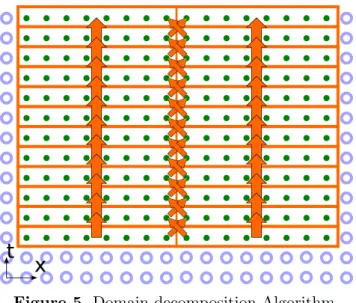
For single-precision, to move the problem closer to the compute-bound domain, the arith-metic intensity should be increased. For this purpose, we propose a Recursive Domain Decom-position (RDD) algorithm to localize the cell data in the SM registers. The classical Domain Decomposition (Fig. 5) divides the computing domain into equal domains, and each domain is assigned to its processor element. The local memory of that processor element stores unk−1 and unk layer data for its domain, and the element computes cell updates for them layer by layer. Each step it exchanges data with the neighboring elements.
Figure 5.Domain decomposition Algorithm
However, one device contains at least 2 levels of parallelism, SM and CUDA threads. Thus, we choose to implement 2-level RDD (Fig. 6). This approach is close to the tiling (blocking) methods, such as [9], since the performance gain is achieved by the use of the faster memory for each process.
t
x
Figure 6. Two-level Recursive Domain Decomposition (RDD) Algorithm. Domains of the first
level are outlined in blue, domains of the second level are outlined in orange
3.1. Synchronization
For the data exchange between SMs the L2 cache is used, and for the data exchange between threads the shared memory is used. The inter-block synchronization was an open issue up to the release of CUDA 9. Since CUDA 9 for devices with Compute Capability 6.1 or higher, CUDA Cooperative Groups (CG) is an universal API for synchronization [15]. It may be applied to a group of threads of arbitrary size, from one warp to all threads of several devices, situated on one node. This is a barrier synchronization, that is, a chosen group of threads is synchronized altogether. This mechanism seems convenient for our purposes, and we have applied it to our code.
Along with it, we choose to manually implement and test the performance gain of the local block synchronization with a semaphore, the classic synchronization primitive. The semaphore limits the number of parallel processes that can read and write the shared data. In this case two neighboring blocks work with the same data: one reads and the other writes. The pointer array stores the semaphores, assigned to the data section which is subject to the racing condition. The length of the array is equal to twice the number of blocks, since each domain has two regions, which are accessed by other blocks: at the start and at the end. The semaphore data type is integer and it has two states: READABLE (0)andWRITEABLE (1). Before reading the data chunk from the other block, the corresponding semaphore is checked to beREADABLE, usingwhileloop terminated by a semicolon. After the read from memory, the valueWRITABLEis written into the semaphore, since no other block requires this data. The data can now be overwritten by the adjacent block.
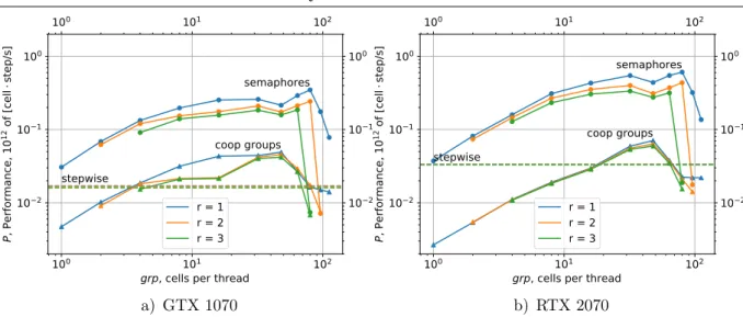
CUDA CG synchronization appears to be inefficient for our problem (see the comparison in Fig. 7). It is the possible reason that the synchronization is called for the whole grid of blocks at once, and all SMs are synchronized. This is superfluous for ensuring the correctness of the data read. Actually, it is sufficient to wait only for the two blocks (in 1D) to complete the work up to this point. If the synchronization of one block with only its neighbors was implemented in CG, it would possibly lead to the acceleration of the memory access.
3.2. Performance Testing
The RDD algorithm is defined by the three parameters: the number of cells per thread
grp, the number ofthreadsin a block and the number of blocks. The number of the domains of the first level of the decomposition is equal to the number of threads, the number of the domains of the second level is equal to the number of blocks. The latter is equal to or divisible by the number of SM in GPU. In the tests we take the maximum possible number of cells, thus
grp·threads·blocks≈const, any two of the parameters may be varied. We have tested various
threads and blocksparameters. “Heavy” blocks and threads, that is, the blocks that use so much shared memory and register space that it may be assigned to an SM only one-by-one, have proven to be more efficient. We fix the number of threads per block to 256, since it is preferable to use all of the 2562 = 65536 registers, and the CUDA compiler does not allow more than 256 registers per thread.
In Fig. 7 the dependency ofPon grpis shown withthreads= 256 and maximum possible
100 100 101 101 102 102
grp, cells per thread
10 2 10 2
10 1 10 1
100 100
P, Pe rfo rm an ce , 1 0
12 of
[c ell ste p/ s] coop groups semaphores stepwise
r = 1 r = 2 r = 3
a) GTX 1070
100 100 101 101 102 102
grp, cells per thread
10 2 10 2
10 1 10 1
100 100
P, Pe rfo rm an ce , 1 0
12 of
[c ell ste p/ s] coop groups semaphores stepwise
r = 1 r = 2 r = 3
b) RTX 2070
Figure 7.Performance dependency on the number of cells per threadgrpparameter in the RDD
algorithm
performance hardly exceeds the performance of the stepwise algorithm. In the following we use only the manual synchronization method with semaphores.
Lowgrpprovide less performance. The performance grows linearly up togrp = 32. Forgrp
in the 32÷80 range the performance shows little variation. It shows that the performance of the code with grp = 32 and 2 blocks per SM and the performance of the code with grp = 64 and 1 block per SM are close. As grp exceeds some peak value, 64 or 80, the abrupt fall of performance is seen. At this point, the data could not be localized in the registers, and register spilling [3] occurs.
In total, the obtained performance is PRDD ∼(300÷600)·109, depending on the stencil radius r.
3.3. Roofline Model
Since the two memory levels are engaged in the RDD algorithm, the two bandwidths are to be considered. Thus, the Roofline is first defined by
Πalg≤min(Πpeak,ΘL2·Ialg,L2,Θsh·Ialg,sh). (5)
Here the denominations are as in section 2.2, and the extra subscript denotes the type of memory (L2 cache or shared). As before, Oalg = (2r + 1) cellFMA·step. The data throughput is estimated as follows. In each block, there aregrp·threadscells. Each block exchanges 4rvalues of 4B size. Thus, assuming grp= 64 and threads= 256,
Dalg,L2 =
4r
grp·threads·4
B cell·step ∼
r 1000
B cell·step.
Similarly, each thread has grpcells and exchanges 4r values,
Dalg,sh= 4r
grp·4
B cell·step ∼
r 16
10 1 10 1 100 100 101 101 102 102
Ialg, operational intensity, FMA/B
102 102
103 103
104 104
alg , p er fo rm an ce , G FM A/ s
r = 1 r = 2 r = 3
a) GTX 1070
10 1 10 1 100 100 101 101 102 102
Ialg, operational intensity, FMA/B
102 102
103 103
104 104
alg , p er fo rm an ce , G FM A/ s
r = 1 r = 2 r = 3
b) RTX 2070
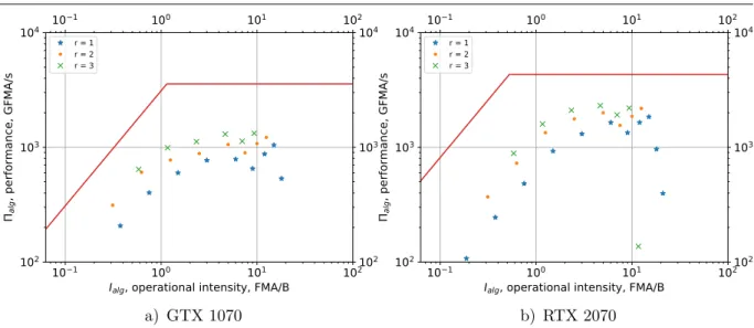
Figure 8. The Roofline model against shared memory bandwidth for the RDD algorithm
The operational intensity is
Ialg= Oalg Dalg ∼
1000·2rr+1 FMAB ,inter-block via L2 cache 16·2r+1
r FMA
B ,inter-thread via shared memory .
Table 3. GPU characteristics: α is the shared memory efficiency, µ is the number of SM,
ϕ is the number of shared memory banks per SM,β is the bank width,νgr is the graphics clock rate, Θsh is the shared memory bandwidth
GPU α µ [SM] ϕ[bankSM ] β [clockB·bank] νgr [Gclocks ] Θsh =αµϕβνgr [GBs ]
GTX 1070 0.85 15 32 4 1.911 3118
RTX 2070 0.85 36 32 4 2.100 8225
The shared memory bandwidth may be calculated as Θsh =αµϕβνgr, all these parameters and their descriptions are gathered in Tab. 3. The L2 cache bandwidth may be estimated as ΘL2= (3÷5)Θ [2], where Θ is taken from Tab. 2.
Now, it is easy to see that Θsh·Ialg,sh ΘL2 ·Ialg,L2 on actualthreads values, therefore the inequality (5) can be reduced to
Πalg ≤min(Πpeak,Θsh·Ialg,sh). (6)
The Roofline model (6) is plotted in Fig. 8. The markers show the performance for different values of grp. The color of a marker signifies the value of r.
The resulting performance for highest points is about 50% of the theoretical peak value. This result was obtained by localization of data in the registers and “heavy” blocks and threads (grp1)
4. Recursive Domain Decomposition with Halo
Further increase in performance seems to be impeded by the high latency of L2 cache. This fact prevents the complete use of the L2 memory bandwidth. This may be mitigated by the introduction of a halo of redundant compute [20, 30].
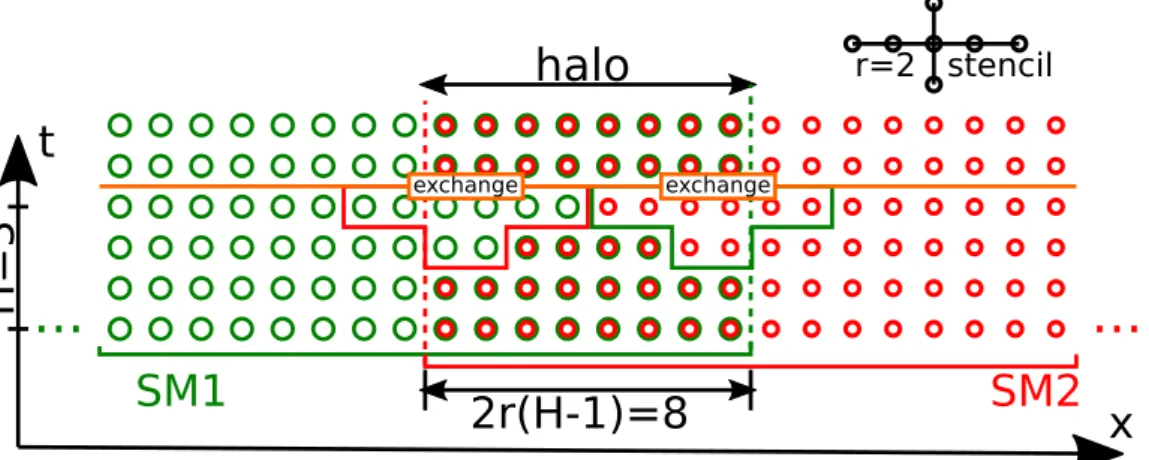
The key idea of halo is simple: instead of the exchange of D data each step, the exchange of ∼ H·D data each H steps takes place (Fig. 9), that is a kind of temporal tiling. Since the data is required in each step for correct simulation, the domains are overlapped.
SM1
t
x
SM2
H=3
2r(H-1)=8
...
...
r=2 stencil
exchange exchange
halo
Figure 9.RDDHalo algorithms on the dependency graph. The cells that are computed correctly
and stored on the two adjacent SM are shown in two colors. The data that should be sent in the synchronization is outlined in colored boxes
In the overlapped domain (halo) on the interface of two SMs, the cells are updated on both SMs (Fig. 9). At start, both SMs store the correct values of all cells, that are assigned to be updated on them, and r more values at each side that are required for the update. After the first update, the data is not enough, so r cells on each side of the domain are incorrect after the second update. The number of correct values is decreased in each step between the synchronization events eachHtime steps. Then, the data exchange takes place to actualize both domains. The size of the halo is 2r(H−1). The data to be exchanged are the cells of the half of the halo, and the r more values that are necessary for the stencil computation on the next step, 2r(H2−1) +r total. Since the stencil requires two time layers, 2r(H2−1) −r more values are required from the previous time step. The data required for the exchange from the two time steps is outlined by theexchange box in Fig. 9.
Although the halo was implemented both for inter-thread (Hb) and inter-block (Hg) in-terfaces, only the inter-block halo has a significant influence on the performance. The shared memory latency is low enough so that Hb = 1 (no halo) or Hb = 2 is enough to completely conceal it.
4.1. Roofline Model
The operational intensity is twice lower than in the RDD algorithm, since two time layers are exchanged each time. Nevertheless, it is still high enough for the problem to be compute-bound.
On the other hand, the latency overhead limits the performance. We may write
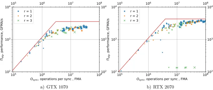
Πalg≤min(Πpeak,ΘL2Ialg,L2,ΘshIalg,sh, Osync/Λsync), (7)
where Osync = KHOalg is the operation count between synchronizations, K is the number of cells, Λsync = min
r,grptstepis the inter-block synchronization time, wheretstepis the elapsed time to perform one step of RDD algorithm (Hg= 1). Λsync = 0.84µs and Λsync = 0.90µs for GTX 1070 and RTX 2070, respectively. The Πpeak and Osync/Λsync limits are visualized as a Roofline in Fig. 10. The markers show the performance of our implementation for different values ofgrp, Hg and Hb. The graph confirms the attention to the latency overhead, and the fact that it is overcome with the introduction of halo.
105 105
106 106
107 107
108 108
Osync, operations per sync , FMA
102 102
103 103
104 104
alg
, p
er
fo
rm
an
ce
, G
FM
A/
s
r = 1 r = 2 r = 3
a) GTX 1070
105 105
106 106
107 107
108 108
Osync, operations per sync , FMA
102 102
103 103
104 104
alg
, p
er
fo
rm
an
ce
, G
FM
A/
s
r = 1 r = 2 r = 3
b) RTX 2070
Figure 10.Latency limitation. The markers show the results of the test runs with different halo
and grpparameters. Larger marker corresponds to larger Hg
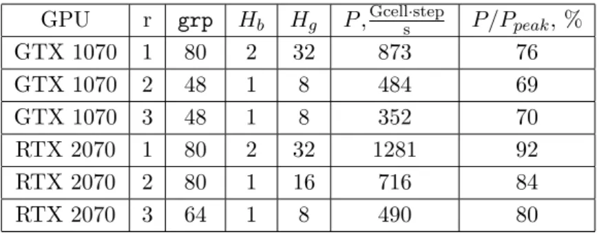
The highest performance we achieved and the parameters that were used are presented in Tab. 4.
Conclusion
Table 4.The highest performance results obtained with RDDhalo
GPU r grp Hb Hg P,Gcells·step P/Ppeak, %
GTX 1070 1 80 2 32 873 76
GTX 1070 2 48 1 8 484 69
GTX 1070 3 48 1 8 352 70
RTX 2070 1 80 2 32 1281 92
RTX 2070 2 80 1 16 716 84
RTX 2070 3 64 1 8 490 80
that the implementation has minimal overhead and that the Roofline estimation was correct. We have found a way to get a performance of more than 90% of the compute-bound limitation, and more than 80% for larger stencil radius.
According to our previous experience, in the practice of implementation of codes in scientific computing, the omnipresent issue is to evaluate the progress on performance optimization. That is, whether the code has reached the performance limit, or it may be further improved by increasing the operational intensity, utilizing better programming tools, reducing overhead. The impact of the current paper is the evidence that the stencil codes performance may be driven close to the peak if the computations are localized in the highest level of the memory hierarchy of GPU, namely in the register file. In the stepwise implementation, the obtained efficiency value is ∼ 1010 cell·sstep, and in the RDDhalo algorithm, it is ∼ 1012 cell·sstep. Both correspond closely to the Roofline estimate. The RDDhalo performance is compute-bound and reaches 92% of the peak computing performance.
We assume that it is the computing performance peak limit in any further stencil codes implementations. Such codes are relevant, for example, in electromagnetic wave simulation with the FDTD method, elastic wave simulation with the Levander scheme. More complex multi-level numerical schemes often use the cross stencil as one of the computation stages as well [17]. As is, the wave equation simulation is used both in optics and in seismic codes. In case the purpose of the simulation is the solution of inverse problem, such as image reconstruction in seismic exploration, double precision is excessive and single precision will suffice.
Any other stencil code, including the 3D extension of the current scheme, is more complex than the one used in this work. So the obtained performance efficiency value is unlikely to be surpassed on the current hardware. The data size in the problem fits the register file, which is comparatively small. However, the common trend in newer GPU is the increase of the register file space. It is 3.75 MB on Kepler, 6 MB on Maxwell, 14 MB on Pascal, 20 MB on Volta [16].
This paper is distributed under the terms of the Creative Commons Attribution-Non Com-mercial 3.0 License which permits non-comCom-mercial use, reproduction and distribution of the work without further permission provided the original work is properly cited.
References
1. De Donno, D., Esposito, A., Tarricone, L., Catarinucci, L.: Introduction to GPU computing and CUDA programming: A case study on FDTD [EM programmer’s notebook]. IEEE An-tennas and Propagation Magazine 52(3), 116–122 (2010), DOI: 10.1109/MAP.2010.5586593
2. Jia, Z., Maggioni, M., Smith, J., Scarpazza, D.P.: Dissecting the NVidia Turing T4 GPU architecture via microbenchmarking. arXiv: 1903.07486 (2019)
3. Jia, Z., Maggioni, M., Staiger, B., Scarpazza, D.P.: Dissecting the NVidia Volta GPU architecture via microbenchmarking. arXiv: 1804.06826 (2018)
4. Hou, K., Wang, H., Feng, W.c.: GPU-unicache: Automatic code generation of spa-tial blocking for stencils on GPUs. In: Proceedings of the Computing Frontiers Confer-ence, May 15–17, 2017, Siena, Italy. pp. 107–116. ACM, New York, NY, USA (2017), DOI: 10.1145/3075564.3075583
5. Endo, T.: Applying recursive temporal blocking for stencil computations to deeper memory hierarchy. In: 2018 IEEE 7th Non-Volatile Memory Systems and Applications Symposium (NVMSA), Hakodate, Japan, August 28-31, 2018. pp. 19–24. IEEE (2018), DOI: 10.1109/N-VMSA.2018.00016
6. Wolf, M.E., Lam, M.S.: A data locality optimizing algorithm. In: ACM Sigplan Notices. vol. 26, pp. 30–44. ACM (1991)
7. Barba, L.A., Yokota, R.: How will the fast multipole method fare in the exascale era. SIAM News 46(6), 1–3 (2013)
8. Yount, C., Duran, A.: Effective use of large high-bandwidth memory caches in HPC stencil computation via temporal wave-front tiling. In: 2016 7th International Workshop on Per-formance Modeling, Benchmarking and Simulation of High PerPer-formance Computer Systems (PMBS). pp. 65–75. IEEE, Salt Lake, UT, USA (Nov 2016), DOI: 10.1109/PMBS.2016.012
9. Datta, K., Murphy, M., Volkov, V., Williams, S., Carter, J., Oliker, L., Patterson, D., Shalf, J., Yelick, K.: Stencil computation optimization and auto-tuning on state-of-the-art multicore architectures. In: Proceedings of the 2008 ACM/IEEE conference on Supercom-puting, Austin, Texas November 15-21, 2008. pp. 4:1–4:12. IEEE Press, Piscataway, NJ, USA (2008), DOI: 10.1109/SC.2008.5222004
10. Rawat, P.S.: Optimization of stencil computations on GPUs. Ph.D. thesis, The Ohio State University (2018)
12. Prokop, H.: Cache-oblivious algorithms. Ph.D. thesis, Massachusetts Institute of Technology (1999)
13. Nguyen, A., Satish, N., Chhugani, J., Kim, C., Dubey, P.: 3.5-D blocking optimization for stencil computations on modern CPUs and GPUs. In: Proceedings of the 2010 ACM/IEEE International Conference for High Performance Computing, Networking, Storage and Anal-ysis, New Orleans, Louisiana, November 13-19, 2010. pp. 1–13. IEEE Computer Society (2010), DOI: 10.1109/SC.2010.2
14. Fukaya, T., Iwashita, T.: Time-space tiling with tile-level parallelism for the 3D FDTD method. In: Proceedings of the International Conference on High Performance Computing in Asia-Pacific Region, Chiyoda, Tokyo, Japan, January 28-31, 2018. pp. 116–126. HPC Asia 2018, ACM, New York, NY, USA (2018), DOI: 10.1145/3149457.3149478
15. NVIDIA Corporation: CUDA C programming guide. https://docs.nvidia.com/cuda/ pdf/CUDA_C_Programming_Guide.pdf (2019), pG-02829-001 v10.1, accessed: 2019-06-18
16. NVIDIA Corporation: NVIDIA Tesla V100 GPU architecture. the worlds most ad-vanced data center GPU. https://images.nvidia.com/content/volta-architecture/
pdf/volta-architecture-whitepaper.pdf(2017), wP-08608-001 v1.1, accessed: 2019-06-18
17. Korneev, B., Levchenko, V.: Detailed numerical simulation of shock-body interaction in 3D multicomponent flow using the RKDG numerical method and DiamondTorre GPU algorithm of implementation. In: Journal of Physics: Conference Series. vol. 681, p. 012046. IOP Publishing (2016), DOI: 10.1088/1742-6596/681/1/012046
18. Zakirov, A., Levchenko, V., Perepelkina, A., Zempo, Y.: High performance FDTD algorithm for GPGPU supercomputers. In: Journal of Physics: Conference Series. vol. 759, p. 012100. IOP Publishing (2016), DOI: 10.1088/1742-6596/759/1/012100
19. Fornberg, B.: Generation of finite difference formulas on arbitrarily spaced grids. Mathe-matics of computation 51(184), 699–706 (1988)
20. Maruyama, N., Aoki, T.: Optimizing stencil computations for NVIDIA Kepler GPUs. In: Proceedings of the 1st International Workshop on High-Performance Stencil Computations, January 21, 2014, Vienna, Austria. pp. 89–95
21. Williams, S., Waterman, A., Patterson, D.: Roofline: an insightful visual performance model for multicore architectures. Communications of the ACM 52(4), 65–76 (2009), DOI: 10.1145/1498765.1498785
22. Quiller´e, F., Rajopadhye, S., Wilde, D.: Generation of efficient nested loops from polyhedra. International journal of parallel programming 28(5), 469–498 (2000), DOI: 10.1023/A:1007554627716
24. Phillips, E.H., Fatica, M.: Implementing the Himeno benchmark with CUDA on GPU clusters. In: 2010 IEEE International Symposium on Parallel & Distributed Processing (IPDPS), April 19-23 2010, Atlanta, GA, USA. pp. 1–10. IEEE (2010), DOI: 10.1109/IPDPS.2010.5470394
25. Levchenko, V.D.: Asynchronous parallel algorithms as a way to archive effectiveness of computations. Journal of Inf. Tech. and Comp. Systems (1), 68 (2005), (in Russian)
26. Levchenko, V.D., Perepelkina, A.Y.: Locally recursive non-locally asynchronous algo-rithms for stencil computation. Lobachevskii Journal of Mathematics 39(4), 552–561 (2018), DOI: 10.1134/S1995080218040108
27. Muranushi, T., Makino, J.: Optimal temporal blocking for stencil computation. Procedia Computer Science 51, 1303–1312 (2015), DOI: 10.1016/j.procs.2015.05.315
28. Muranushi, T., Nishizawa, S., Tomita, H., Nitadori, K., Iwasawa, M., Maruyama, Y., Yashiro, H., Nakamura, Y., Hotta, H., Makino, J., et al.: Automatic generation of ef-ficient codes from mathematical descriptions of stencil computation. In: Proceedings of the 5th International Workshop on Functional High-Performance Computing, Nara, Japan, September 22, 2016. pp. 17–22. ACM, New York, NY, USA, DOI: 10.1145/2975991.2975994
29. Riesinger, C., Bakhtiari, A., Schreiber, M., Neumann, P., Bungartz, H.J.: A holistic scalable implementation approach of the lattice Boltzmann method for CPU/GPU heterogeneous clusters. Computation 5(4), 48 (2017), DOI: 10.3390/computation5040048
30. Holewinski, J., Pouchet, L.N., Sadayappan, P.: High-performance code generation for stencil computations on GPU architectures. In: Proceedings of the 26th ACM international confer-ence on Supercomputing, San Servolo Island, Venice, Italy June 25-29, 2012. pp. 311–320. ACM, DOI: 10.1145/2304576.2304619
31. Krotkiewski, M., Dabrowski, M.: Efficient 3D stencil computations using CUDA. Parallel Computing 39(10), 533–548 (2013), DOI: 10.1016/j.parco.2013.08.002