Some applications of linear difference equations in finance with wolfram|alpha and maple

(1)

Some applications of linear difference

equations in finance

with wolfram

|

alpha and maple

Dana ˇ

R´ıhov´

a, Lenka Viskotov´

a

Department of Statistics and Operation Analysis,

Faculty of Business and Economics,

Mendel University in Brno, Zemˇedˇelsk´a 1, 613 00 Brno

[email protected],[email protected]

Abstract

The principle objective of this paper is to show how linear differ-ence equations can be applied to solve some issues of financial mathe-matics. We focus on the area of compound interest and annuities. In both cases we determine appropriate recursive rules, which constitute the first order linear difference equations with constant coefficients, and derive formulas required for calculating examples. Finally, we present possibilities of application of two selected computer algebra systems Wolfram|Alpha and Maple in this mathematical area.

Key words: linear difference equation, compound interest, future value of an annuity, periodic payment, computer algebra systems.

2000 AMS: 39A06, 39-04.

1 Introduction

(2)

Many formulas used in financial mathematics can be derived from the recursive rules between two consecutive elements which constitute difference equations of the first order. This includes for example simple and compound interest calculation, the present and future value of an annuity and loan amortization.

2 Compound Interest

2.1 Derivation of Formula

A sum of money deposited in a bank earns interest which is added to the principal at regular intervals and the new amount is used for calculating the interest for the next conversion period. We shall develop a formula for the total amount of money that is accumulated by a given principal after a certain number of conversion periods, see also [3], [4].

Let r stand for the annual interest rate and k denote the number of conversion periods in a year. Let n be equal to the number of conversion periods in the term of the deposit. Let yn represent the amount on deposit at the end of n conversion periods and P the initial sum deposited (i.e. principal). We obtain the following recursive rule

yn+1 =yn+ r kyn=

1 + r

k

yn, n = 0,1,2, . . .

withy0 =P, where the fraction _kr stands for the interest rate per conversion

period and _krynis the interest generated during (n+1)st period. The previous formula represents the first order homogeneous linear difference equation with constant coefficients

yn+1−

1 + r

k

yn= 0 (1)

with initial condition

y0 =P. (2)

The above problem (1), (2) can be solved by using the properties of a geo-metric sequence, see [1] and [8]. But our approach will be different due to the use of a difference equation. The characteristic equation of (1) takes form

z−1 + r k

= 0 with real root

(3)

According to [5], the general solution is a geometric sequence yn =C

1 + r

k n

, C ∈_R.

A constantC can be specified from the initial condition (2) for periodn= 0, hence

C =P. Thus the general solution is given by

yn =P

1 + r k

n

(3) and represents the compound interest formula. This formula gives the amount yn into which principalP grows when it earns compound interest forn con-version periods at an interest rate of r_k per conversion period.

2.2 Illustrative Examples

Example 2.1. An amount of EUR 1,000 is deposited into a savings account

at an annual interest rate of 2.5%, compounded yearly. What will the value of the account be worth after 20 years?

To find the amount we use formula (3). We have principalP = 1,000, annual interest rate r = 0.025, number of conversion periods per year k = 1 and total number of conversion periodsn = 20. After plugging those figures into the formula, we get

y20= 1000

1 + 0.025 1

20 .

= 1638.62

Example 2.2. Find the number of years required for a given sum of money

to double itself if the interest rate is 3%, compounded quarterly.

Substituting yn = 2P in the compound interest formula (3), we have 2P =P 1 + r

k n

which implies

2 = 1 + r k

n

. (4)

Taking natural logarithms on both sides and using properties of logarithms gives

n= ln 2 ln 1 + r

(4)

To calculate the number of years N we have to divide the total number of conversion periods n by their number in a yeark

N = 1 k

ln 2

ln 1 + _kr. (5)

Settingr = 0.03, k = 4 we get the required number of years N = 1

4

ln 2 ln 1 + 0.₄03

. = 23.19

3 Future Value of an Annuity

3.1 Derivation of Formula

An annuity is essentially a sequence of periodic payments, usually equal in amount, payable at equal intervals of time over the course of a fixed time period. The future value of an annuity is the total value of its periodic payments enhanced at interest rate for given number of conversion periods. It is defined as the sum of the amounts of all payments and the total compound interest earned on these payments to the time of the last payment. See for example [1], [4].

Suppose the constant sum R is deposited at the end of each conversion period in a bank which credits interest at the annual rater. The deposits are made k times each year over n conversion periods. Let yn denote the total amount in the account at the end of n conversion periods. We shall find the total worth of an annuity after n deposits.

The recursive rule for the future value of an annuity can be written as yn+1 =yn+

r

kyn+R =

1 + r k

yn+R, n= 0,1,2, . . . with y0 = 0, where r_k is the interest rate per conversion period.

This equation constitutes the first order nonhomogeneous linear difference equation with constant coefficients

yn+1−

1 + r

k

yn =R (6)

with initial condition

y0 = 0. (7)

(5)

difference equations like in the case of compound interest. To solve nonhomo-geneous difference equation (6) we consider the corresponding homononhomo-geneous difference equation

yn+1−

1 + r

k

yn= 0 (8)

which is the same as (1) in the case of compound interest. Hence the general solution ¯yn of this homogeneous difference equation is given by

¯ yn =C

1 + r

k n

, C ∈_R. (9)

The right-hand side of the nonhomogeneous difference equation (6) is a con-stant R which is a polynomial of degree zero. Thus a particular solution Yn can be estimated by

Yn =b, b ∈R.

For more details see [5]. Using the method of undetermined coefficients (see [2]) we substitute the above estimate into (6). We get

b−1 + r k

b=R and solving for b we obtain

b =−Rk r.

Therefore the particular solution of (6) takes the form

Yn =−R k

r. (10)

Using (9), (10) according to the superposition principle (see [6]), the general solution of the nonhomogeneous linear difference equation (6) is the sum

yn =Yn+ ¯yn =−R k r +C

1 + r

k n

, C ∈_R.

A constantC can be specified from the initial condition (7) for periodn= 0. Hence we obtain

C =Rk r.

Consequently, the general solution of (6) takes the form

yn=−R k r +R

k r

1 + r

(6)

which can be written as

yn=R

1 + _krn−1 r k

. (11)

The above relation represents the future value of an annuity formula which gives the amount of an annuity ofn payments of R at the compound rate r_k per conversion period under the assumption that the payment interval equals the conversion period. The future value of an annuity formula is used to calculate what value at a future date would be for a series of periodic payments.

In financial mathematics, it is common to use the following form of the formula (11) settingi= r

k whereirepresents the interest rate per compound-ing interval (see [8] and [10])

yn =R

(1 +i)n−1

i . (12)

3.2 Illustrative Examples

Example 3.1. Suppose EUR 500 is deposited at the end of every six-month

period in a bank, whose annual rate is3.4%, compounded semiannually. How much will this account be worth after 7 years?

We get the solution using (11), where R = 500, r = 0.034, k = 2, n = 14. Then we obtain

y14= 500

1 + 0.034 2

14 −1

0.034 2

.

= 7828.64

Example 3.2. Find the payment amount that you should deposit at the end

of each month in a bank so that EUR 35,000 will be available after 10 years if the interest rate is 1.6%, compounded monthly after each deposit.

Solving for R from the future value of an ordinary annuity formula (11) we get

R =yn

r k

1 + _krn−1.

In our case we have r = 0.016, k = 12, n = 120, y120 = 35,000. Hence the

monthly payment is calculated as follows R= 35,000

0.016 12

1 + 0.₁₂016120−1 .

(7)

4 Solving with Computer Algebra Systems

In mathematics of finance, Excel is commonly used for calculations. In this paper the quoted calculations of compound interest and annuitity are completed by computational tool Wolfram|Alpha and mathematical software Maple, respectively.

4.1 Wolfram

|

Alpha

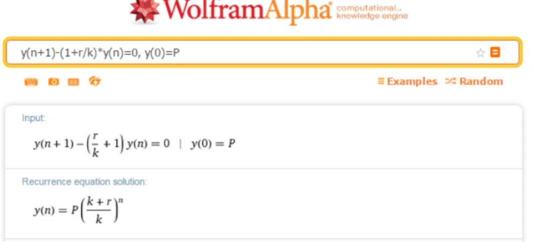
We will demonstrate the computation of compound interest (3) and Ex-ample 2.2 through the free online service Wolfram|Alpha, which is available via any web browser at http://wolframalpha.com. This tool provides math-ematical computations based on software Mathematica and accepts com-pletely free-form input, commands are specified by the name of operation in English.

To solve the difference equation (1) with the initial condition (2) we type both equations together separated by comma into an input field writing in-dexes in parentheses. The provided general solution (3) is shown in Figure 1.

Fig. 1. Compound interest formula

(8)

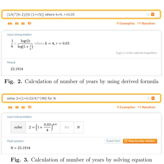
Fig. 2. Calculation of number of years by using derived formula

Fig. 3. Calculation of number of years by solving equation

4.2 Maple

Now we show the computation of the future value of an annuity (11) and illustrative Example 3.2.

We assign the recurrence relation (6) to the nameREq. > REq:=y(n+1)-y(n)*(1+r/k)=R;

Maple returns the output:

REq :=y(n+ 1)−y(n)

1 + r k

=R

Then we make the assignment of the initial condition (7) to the name IC. > IC:=y(0)=0:

(9)

parentheses.

> rsolve({REq,IC},y(n));

Rk k+_krn

r −

kR r

The above obtained expression corresponds to the future value of an annuity (11).

For determining the payment R we type the following command, where F V equals to the total amount yn in the account upon the last deposit (i.e the future value of an annuity).

> isolate(%=FV,R):simplify(%);

R = F V r k k+_krn−1

To make the calculation of Example 3.2 we use command subs. > subs(k=12,r=0.016,FV=35000,n=120,%);

R = 269.1493510

4.3 Comparison of Used Systems

The professional Maple is very powerful tool which enables to make new procedures and modules, save and read them or together with other data store in a library. On the other hand, it requires certain programming skills. In comparison with Maple, Wolfram|Alpha does not allow to save and reload the results of computations and make own procedures, also its perfor-mance is rather slow. But its significant advantage is that it is free online and very simple to use. Moreover, Wolfram|Alpha provides a variety of com-putations from other fields, for example from money and finance.

5 Conclusion

This paper has discussed linear difference equations and their applications in economics (see also [9]). These equations are frequently used especially in financial mathematics and some of their typical applications have been presented here.

(10)

of an annuity formula by means of solution of difference equations. The simultaneous application of mathematical software has been demonstrated, the supplementary computations have been performed through Maple and Wolfram|Alpha.

Finally, the paper emphasizes the need for mathematics in economic sub-jects. The presented approach can be used in teaching of mathematics at economic universities and helps to provide students with the opportunities to apply their mathematics in relevant economics contexts.

References

[1] J. J. Costello, O. S. Gowdy and M. A. Rash, Mathematics for the Man-agement, Life, and Social Sciences, New York: Harcourt Brace Jo-vanovich, Inc., 1982.

[2] S. Elaydi, An Introduction to Difference Equations, New York: Springer Science+Business Media, Inc., 2005.

[3] G. Fulford, P. Forrester and A. Jones, Modelling with Differential and Difference Equations, Cambridge: Cambridge University Press, 1997. [4] S. Goldberg,Introduction to Difference Equations: With Illustrative

Ex-amples from Economics, Psychology and Sociology, New York: Dover Publications, Inc., 2010.

[5] J. Mouˇcka and P. R´adl, Matematika pro studenty ekonomie, Praha: Grada Publishing, Inc., 2010.

[6] K. Neusser, Difference Equations for Economists, Bern: Univer-sity of Bern, 2012, [Online], [Cited 2015-07-15]. Available from: http://www.neusser.ch/downloads/DifferenceEquations.pdf.

[7] P. Praˇzák,Diferenˇcn´ı rovnice s aplikacemi v ekonomii, Hradec Králové: Gaudeamus, 2013.

[8] J. Radová, P. Dvoˇrák and J. Málek, Finanˇcn´ı matematika pro kaˇzdého, Praha: Grada Publishing, Inc., 2005.

[9] D. ˇR´ıhov´a and L. Viskotov´a, Compound Interest and Annuities with Linear Difference Equations and CAS, MITAV 2015 (proceedings of ab-stracts), Brno: University of Defence, 2015.