INTIMATE RELATIONSHIP SATISFACTION AND DEMAND-WITHDRAW TRAJECTORIES: UNDERSTANDING DEVELOPMENT IN NEWLYWED COUPLES
Jennifer M. Belus
A thesis submitted to the faculty at the University of North Carolina at Chapel Hill in partial fulfillment of the requirements for the degree of Masters of Arts in the Department of Psychology (Clinical) in the School of Arts and Sciences.
Chapel Hill 2015
ABSTRACT
Jennifer M. Belus: Intimate Relationship Satisfaction and
Demand-Withdraw Trajectories: Understanding Development in Newlywed Couples (Under the direction of Donald Baucom)
ACKNOWLEDGMENTS
TABLE OF CONTENTS
LIST OF TABLES……….……vi
LIST OF FIGURES……….…..vii
LIST OF ABBREVIATIONS………..viii
CHAPTER 1: INTRODUCTION………1
CHAPTER 2: METHOD………...11
Participants and Procedure……….11
Measures………....12
Data Analytic Plan……….13
CHAPTER 3: RESULTS………...16
Hypothesis 1………...19
Hypothesis 2………...25
Hypothesis 3………...26
Hypothesis 4………...35
CHAPTER 4: DISCUSSION……….41
APPENDIX 1: UNIVARIATE MODEL PARAMETER ESTIMATES OF RELATIONSHIP SATISFACTION FOR HUSBANDS AND WIVES………...53
APPENDIX 2: UNIVARIATE MODEL PARAMETER ESTIMATES OF DEMAND-WITHDRAW FOR HUSBANDS AND WIVES………...54
LIST OF TABLES
Table 1 – Means for relationship satisfaction and demand-withdraw for
husbands and wives………17 Table 2 – Within-person and cross-partner correlations………18 Table 3 – Hypothesis 1— Multivariate model parameter estimates of
relationship satisfaction for husbands and wives………...23 Table 4 – Hypothesis 2— Multivariate parameter estimates of relationship
satisfaction using husbands and wives’ intercepts as a predictor of partner
slopes………..27 Table 5 – Hypothesis 3— Multivariate model parameter estimates of
relationship satisfaction and demand-withdraw for husbands………...29 Table 6 – Hypothesis 3—Multivariate model parameter estimates of
relationship satisfaction and demand-withdraw for wives………33 Table 7 – Hypothesis 4—Multivariate model parameter estimates of
husbands’ relationship satisfaction with wives’ demand-withdraw………..37 Table 8 – Hypothesis 4—Multivariate model parameter estimates of
LIST OF FIGURES
LIST OF ABBREVIATIONS
CFI Comparative fit index
CPQ Communication patterns questionnaire DAS Dyadic adjustment scale
LCGA Latent class growth analysis
RMSEA Root mean squared error of approximation SEM Structural equation modeling
SRMR Standardized root mean square error residual
CHAPTER 1: INTRODUCTION
Understanding intimate relationship satisfaction is a hallmark of couples research, and scholarship in this area has continued to grow. It is not only important to understand whether couples are satisfied or dissatisfied at a given point in time, but also how they have evolved over time to reach their current level of functioning (Karney & Bradbury, 1995). In particular, there might be different paths that result in the same outcome, which is important from an intervention perspective since there may be optimal times to intervene, either to prevent or remediate distress. Thus, elucidating the trajectory of relationship satisfaction is an important research endeavor.
satisfaction showed small but significant linear declines in satisfaction over time, and the group with low levels of initial satisfaction showed larger and more rapid declines over the same period. These distinct trajectories were also found by Kamp Dush, Taylor, and Kroger (2008) using data from the Marital Instability Over the Life Course study (Booth, Johnson, Amato, & Rogers, 2003), where a random national sample of married persons of varying marital duration (M = 12.45 years, SD = 9.16) were followed for 20 years. These studies provide evidence that there is a positive covariance between initial level of relationship satisfaction and rate of change over time. Specifically, those who start off at higher levels of satisfaction show fewer declines over time, but as initial satisfaction decreases, the amount of decline in satisfaction increases (i.e., the slope becomes more negative). These findings are important because they suggest that collapsing couples across different satisfaction levels misrepresents and masks important differences in satisfaction trajectories that appear to exist, depending on the initial level of satisfaction.
One limiting factor in understanding the longitudinal trajectory of relationship
of change over time. Although this more interactive longitudinal approach has not yet been examined, it is generally viewed that having a partner with lower satisfaction is deleterious to the relationship satisfaction of the other partner, whereas having a partner with higher satisfaction is expected to have beneficial effects on the satisfaction of the other partner.
Although the developmental course of relationship satisfaction and the interaction between partners in newlywed couples still needs to be elucidated, one robust finding is that there are certain risk factors that are related to poor relationship satisfaction. One such factor is the type of communication exhibited by couples, often examined in the context of conflict resolution or problem-solving discussions. Numerous studies have shown that negative
interaction patterns between partners have deleterious effects on relationship satisfaction, above and beyond the general negativity expressed by partners (e.g., Baucom, McFarland, &
Christensen, 2010; Bradbury & Karney, 1993; Caughlin & Huston, 2002), and also increase the likelihood of divorce in married couples (e.g., Birditt, Brown, Orbuch, & McIlvane, 2010; Markman & Hahlweg, 1993; Stanley, Markman, & Whitton, 2002).
The demand-withdraw pattern of communication, considered to be a negative
hand, when men desire their partner to change, the pattern of wife-demand/husband-withdraw is equally likely as husband-demand/wife-withdraw (Baucom et al., 2010; Vogel & Karney, 2002). However, it does appear that men and women desire change in their partners at similar levels (Caughlin & Vangelisti, 1999), so greater demandingness in women cannot be completely accounted for by the belief that women have greater desire for their partner to change.
Although a greater understanding of the reasons for the demand-withdraw pattern are needed, a consistent finding is that the presence of this communication pattern is associated with concurrent relationship dissatisfaction for both partners (e.g., Caughlin, 2002; Heavey,
Christensen, & Malamuth, 1995; Kurdek, 1995; Noller, Feeney, Bonnell, & Callan, 1994); however, the longitudinal research examining this association is less consistent. A study by Heavey and colleagues (1995) found that greater wife-demand/husband-withdraw from
be an attempt to problem-solve but rather be used as an avoidance strategy from discussing important problems. In this case, behavior change would not follow, and relationship satisfaction would decline. As a result, the presence of demand-withdraw in newly established relationships, including newlywed couples, is theorized to be more deleterious to relationship functioning.
In addition, the above studies were first attempts at understanding the longitudinal association between demand-withdraw and relationship satisfaction, but these variables were examined at one point in time (i.e., earlier demand-withdraw predicting later relationship satisfaction), rather than as dynamic constructs that themselves change over time. One study by Kurdek (1995) attempted to capture the variable dynamics by using concurrent change scores over a 2-year period in demand-withdraw and relationship satisfaction and found a negative association, such that increases in demand-withdraw were related to declines in relationship satisfaction. Although this study is applauded for attempting to capture the dynamic nature of these constructs, the approach used does not elucidate whether relationship satisfaction and demand-withdraw follow the same developmental trajectory. This is important to understand because mitigating the demand-withdraw pattern is often a target of relationship interventions, with the underlying assumption that reducing this behavior will improve relationship satisfaction. However, if these two variables do not follow the same trajectory, specifically in newlywed couples, there may then be reason to explore other variables that do change in tandem with relationship satisfaction that can in turn become targets of relationship enhancement interventions.
Birditt and colleagues (2010) found that over 16 years of marriage, the frequency of both spouses’ constructive conflict and withdrawal behaviors did not change. Over the same period however, wives, but not husbands, decreased the frequency of their destructive conflict
behaviors, though wives initially endorsed higher levels of destructive behaviors as compared to husbands. Relatedly, other researchers have compared changes in positive and negative
communication in couples considered to be distressed and nondistressed after five years of marriage (Markman, Rhoades, Stanley, Ragan, & Whitton, 2010). The investigators found that both groups self-reported increases in negative communication, but that the increase was significantly greater for the distressed than the nondistressed group. However, this study also used videotaped interactions of the couples problem-solving and found negative communication actually declined in both groups over time, but more so for the nondistressed groups. Thus, there are mixed findings with respect to how negative conflict resolution behaviors change over time, which may also be a function of length of relationship. The Markman and colleagues’ (2010) study is particularly important because it was one of the first to examine how changes in communication relate to different relationship satisfaction outcomes. Although one study has examined trajectories of conflict levels as they relate to trajectories of couple satisfaction using latent classes (Kamp Dush & Taylor, 2012), no study has yet examined whether communication behaviors are actually changing in tandem with relationship satisfaction.
Building upon the investigations discussed above, the purpose of the current study is to understand developmental trajectories of relationship satisfaction and how relationship
will be described in terms of predicting outcomes for husbands, with wives fulfilling the role of the partner in the descriptions to follow. However, predictions based on the model below also hold true for wives.
Overall, the proposed model here suggests that high relationship satisfaction and good communication skills (i.e., low demand-withdraw communication) serve as a resource for both the individual and the partner, and these factors are expected to be protective over time.
Relationship satisfaction and demand-withdraw are thought to be related within-person for husbands at a given time point and change in a similar pattern over time. For newlywed husbands who are well-adjusted in relationship satisfaction and demand-withdraw, they will evidence little change and stay relatively stable in both of these areas over time. On the other hand, for husbands who are less well-adjusted in these domains, they will exhibit greater changes in each of these areas (in a negative direction) over time. Thus, this model suggests a positive association between each variable’s baseline level and its change over time. Conceptually, this idea is consistent with the findings regarding trajectories of relationship satisfaction by Kamp Dush and colleagues (2008) and Lavner and colleagues (2012), but instead of predicting distinct groups, these variables will be examined as continuous in order to maintain consistency with the underlying conceptualization that relationship satisfaction and communication lie on continua. In addition, the trajectory of husbands’ relationship satisfaction is also expected to be influenced by their wives’ initial level of relationship satisfaction, such that wives who themselves have higher initial levels of satisfaction will be a positive influence, whereas wives who have lower initial levels of satisfaction will be a negative influence on husbands’ relationship satisfaction
more change in relationship satisfaction will also have wives whose satisfaction exhibits large changes. Finally, husbands’ relationship satisfaction is also expected to be associated with the communication of wives initially and over time, again with wives who have greater functioning in these domains being facilitative and lower levels of wives’ functioning in these domains having a negative influence on husbands’ relationship satisfaction. The same model is also expected to hold true for wives.
Therefore, derived from this model are four primary research goals, which will be investigated in this study:
2. To explore cross-partner effects of relationship satisfaction. Specifically, the current investigation examines how husbands’ initial level of satisfaction influences the
trajectory of wives’ satisfaction over time. It is hypothesized that husbands with higher levels of initial satisfaction will positively influence wives’ satisfaction trajectories, resulting in wives who have less steeply declining satisfaction trajectories, whereas husbands with lower initial satisfaction levels are expected to negatively influence wives’ satisfaction over time, resulting in wives who have more steeply declining satisfaction trajectories. The same pattern of results is expected when predicting trajectories of husbands’ relationship satisfaction from wives’ initial satisfaction levels.
3. To examine the trajectory (i.e., initial status and change over time) of demand-withdraw communication and its association with the trajectory of relationship satisfaction, within a given individual. First, it is hypothesized that there will be a positive covariance between the initial status of demand-withdraw and its change over time, such that lower levels of demand-withdraw at the outset will be associated with a relatively stable level of
demand-withdraw over time, but as the initial level of demand-withdraw communication increases, there will be more rapid increases in how this variable changes over time. In addition, it is hypothesized that within-person (for both husbands and wives), there will be a negative association between demand-withdraw and relationship satisfaction, both in terms of the initial levels of these variables and how they change over time. More
4. To explore the association between relationship satisfaction of husbands and the demand-withdraw communication of wives. It is hypothesized that across partners, the initial level of husbands’ relationship satisfaction will be negatively associated with the initial level of wives’ demand-withdraw, such that greater levels of husbands’ relationship
CHAPTER 2: METHOD
Participants and Procedure
Participants in this study were engaged couples who participated in a modified version of Prevention and Relationship Enhancement (PREP-WK; Burnett, 1993), a pre-marital workshop program designed to provide couples with skills to enhance and prevent distress in their intimate relationship. Couples (N = 93) were recruited between 1991- 1997 into the study through the church in which they planned to be married. Two churches in a small southeastern community in the U.S. collaborated on the study. Couples had the option of either meeting with their minister for individual pre-marital counseling or participating in the study’s pre-marital workshop program, which took place over the course of a weekend once per year. More details on the procedure and nature of the intervention can be found in the paper by Schilling, Baucom, Burnett, Allen, and Ragland (2003).
Couples completed questionnaires pre- and post-intervention. However, for the purposes of the current investigation, post-intervention data were used as the baseline time-point since it was expected that participating in the intervention might result in an immediate improvement in the variables of interest, making it challenging to model linear trajectories of change. Couples were followed up every year for five years post-intervention; however, in 1997 a decision was made to collect follow-up data only at the 1, 2, and 5-year intervals. Therefore, some cohorts in the sample have fewer data points.
schooling (SD = 1.99), and husbands reported 17.23 years of education (SD = 2.13). In addition, the majority of participants were Caucasian (> 97%). The average length of couple’s relationship was 4.14 years (SD = 2.89) according to wives and 4.04 years (SD = 2.73) according to
husbands. Measures
Relationship satisfaction. Relationship satisfaction was measured using the Dyadic Adjustment Scale (DAS; Spanier, 1976). The DAS is a 32-item self-report measure of intimate relationship distress. Higher scores represent better relationship functioning, with scores below 97 on this measure considered to be indicative of clinical relationship distress. The psychometric properties of this measure have been supported by prior research (Sharpley & Cross, 1982). In the present study, the alpha coefficients ranged from .88 - .92 for husbands and .88 - .93 for wives.
Demand-withdraw communication. The demand-withdraw communication pattern was measured using the Communication Patterns Questionnaire (CPQ; Christensen & Sullaway, 1984). The CPQ is a 35-item self-report measure assessing spousal behavior during three stages of conflict, with each item rated on a Likert scale, ranging from 1 (very unlikely) to 9 (very likely). Demand-withdraw is a specific, dyadic pattern of communication in which one partner pushes for discussion of a problem while the other partner avoids discussion. There are two related subscales: one representing the wife-demand/husband-withdraw subscale and the other representing the husband-demand/wife-withdraw subscale. Previous research has either
“demand” role and for men to be in the “withdraw” role in heterosexual relationships
(Christensen, Eldridge, Catta-Preta, Lim, & Santagata, 2006). In addition, combining the two subscales to generate one demand-withdraw scale often results in the scale having low reliability (Brian Baucom, personal communication, February 18, 2013), and can also mask important differences when women versus men are in the “demand” role. In the current study, the
reliability coefficients for the wife-demand/husband-withdraw scale ranged between .59 - .80 for husbands and between .65 - .80 for wives.
Data Analytic Plan
Structural equation modeling (SEM) was conducted in order to estimate multivariate latent growth curve models to test the hypotheses of interest. Latent growth curve models use repeated assessment measures for outcome variables and identify the average growth curve in a given sample based on the individual trajectories of sample members. SEM provides a highly flexible framework that allows for the simultaneous estimation of multiple growth curves. Specifically, this technique allows for modeling trajectories of change for both husbands and wives simultaneously, without violating the assumption of independence of residuals. The intercepts and slopes of the individual growth curves are random, meaning both of these
Thus, the study goals and hypotheses were examined in the following ways:
Hypothesis 1. In order to model trajectories of relationship satisfaction and determine whether a positive covariance existed between an individual’s initial level of relationship satisfaction and change over time (i.e., higher initial satisfaction is associated with less steep declines over time), a multivariate growth curve model was estimated. This model
simultaneously estimated individual growth curves of relationship satisfaction for both husbands and wives. The covariance parameter estimate of the model tested whether the estimated
intercept and slope of relationship satisfaction was associated for husbands and for wives
(separately). Moreover, the covariance parameter between the estimated slopes for husbands and wives’ relationship satisfaction growth curves was examined to determine whether spouses’ relationship satisfaction was changing together over time.
Hypothesis 2. In order to test the effect of husbands’ initial level of relationship satisfaction on wives’ relationship satisfaction changes over time, the estimated intercept of husbands’ growth curves calculated in Hypothesis 1 was used as a predictor of the estimated slope of wives’ growth curves for relationship satisfaction, also calculated in Hypothesis 1.
Simultaneously, the estimated intercept of wives’ growth curves was used as a predictor of the estimated slope of husbands’ growth curves for relationship satisfaction.
within-person. Then, cross-variable parameters were examined. The covariance between the estimated intercepts for relationship satisfaction and demand-withdraw was examined to determine how these variables were related initially; in addition, the covariance between the estimated slopes for relationship satisfaction and demand-withdraw was also examined to determine how these variables were related over time.
CHAPTER 3: RESULTS
As described above, the hypotheses of interest were examined using multivariate latent growth curve models, wherein the trajectories (both intercept and slope) of two variables were simultaneously estimated within the same model. Prior to fitting a multivariate growth curve model, optimal-fitting models for each individual variable were first determined. Therefore, below, the optimal-fitting model for each individual variable is first presented, followed by the results of the multivariate model. Sample means for the variables at each time point are found in Table 1 and sample correlations are found in Table 2.
Table 1
Means for Relationship Satisfaction and Demand-Withdraw for Husbands and Wives
Relationship satisfaction Demand-withdraw
Husbands M (SD)
Wives M (SD)
Husbands M (SD)
Wives M (SD)
Time 0 119.80 (9.87) n = 86
121.77 (9.25) n = 83
9.59 (5.25) n = 90
9.61 (5.57) n = 90 Time 1 116.27 (10.17)
n = 64
118.90 (10.12) n = 65
10.95 (5.01) n = 65
11.11 (5.99) n = 66 Time 2 115.74 (11.85)
n = 60
117.31 (12.86) n = 64
11.23 (5.36) n = 62
10.91 (5.91) n = 67 Time 3 117.07 (8.63)
n = 21
117.91 (11.03) n = 23
11.07 (5.28) n = 14
11.36 (6.37) n =14 Time 4 114.47 (9.47)
n = 15
117.90 (12.61) n = 15
12.89 (5.23) n = 9
10.44 (4.36) n = 9 Time 5 115.87 (11.59)
n = 45
115.17 (11.42) n = 47
12.08 (4.61) n = 43
11.77 (5.51) n = 50
additional indices are the Tucker-Lewis Index (TLI) and Comparative Fit Index (CFI), and both are considered relative goodness-of-fit indices. Potential values fall between 0 and 1, with higher values representing improved fit relative to a restrictive baseline model where none of the
variables in the model are related to each other. There are no sampling distributions for these indices nor are there universal cutoff values, but traditionally values of .90 have been used to indicate good model fit, although recently values closer to .95 have been taken to indicate good fit. Finally, the standardized root mean square residual, or SRMR, is a measure of the average degree of misfit in the model. Values less than .08 are taken to indicate good fit, although there is no empirical evidence to support this cutoff value.
Table 2
Within-Person and Cross-Partner Correlations
Note. *p< .05,**p< .01, ***p< .001.
Within-person correlations between relationship satisfaction and demand-withdraw
Time 0 Time 1 Time 2 Time 3 Time 4 Time 5
Husbands -.65*** -.46*** -.47*** -.62* -.39 -.54*** Wives -.51*** -.69*** -.54*** -.60* -.68* -.51***
Cross-partner correlations for relationship satisfaction and demand-withdraw
Time 0 Time 1 Time 2 Time 3 Time 4 Time 5
Relationship satisfaction
.54*** .48*** .65*** .77*** .74** .68***
Demand-withdraw
Hypothesis 1
The aim of Hypothesis 1 was to examine the association between the initial status and rate of change for relationship satisfaction, within-person, as well as the association of
relationship satisfaction across partners, both in initial status and rate of change. Separate individual growth curve models for relationship satisfaction were first estimated, for both husbands and wives. Overall for husbands, the univariate model of relationship satisfaction fit very poorly. The Chi-Square test of model fit rejected the null hypothesis that the model fit the data (16) = 47.33, p = .001, suggesting that the model was not a good fit for the data.
Consistent with this, the other indices all suggested poor model fit: the RMSEA = .15 (CI = .10 - .20), CFI = .83, TLI = .84, and SRMR = .71. Taken together, the indices of this model suggest that the model did not fit the data well, and therefore the specific results of the model (e.g., intercept, slope) could not be interpreted.
Similar to husbands, the fit indices for the univariate latent growth curve model for relationship satisfaction for wives were also very poor. More specifically, the Chi
square-distributed likelihood ratio test of model fit rejected the null hypothesis that the model fit the data (16) = 39.39, p = .001, suggesting that the model was not a good fit for the data. Consistent with this, the other indices all suggested poor model fit: the RMSEA = .13 (CI = .08 - .18), CFI = .85, TLI = .86, and SRMR = .61. Again, given the poor indices of model fit the specific results of the model (e.g., intercept, slope) were not interpreted.
data analyses were conducted. Given the strong theoretical and empirical support regarding linear trajectories of change in this population, this approach was intended to provide potentially useful information regarding the cause of the unexpected model misfit and aid in identifying more optimally-fitting models. In order to uncover models with more desirable fit statistics, data plots and modification indices provided through Mplus were used. However, because this approach was exploratory in nature (and data-driven), results should be viewed both cautiously and tentatively. Consistent with the cautionary interpretation of these exploratory models, model results with p values ranging from .050 - .099, often considered “marginally significant” and interpreted, were not interpreted here. Substantive interpretations were only made where p < .05, although marginally significant results have been noted throughout for the reader.
Exploratory findings. For husbands, a better fitting univariate model for relationship satisfaction emerged when data from Time 3 and Time 4 were removed and the residual variance from Time 1 and Time 2 were allowed to covary, and all residual variances were constrained to be equal. Model fit evidenced more acceptable fit to the data: Chi square-distributed likelihood ratio test of model fit (7) = 14.68, p = .04, RMSEA = .11 (CI = .02 - .19), CFI = .94, TLI = .95, and SRMR = .15. For wives, a better-fitting model emerged when data from Time 2 and Time 4 were removed. Model fit indices were as follows: Chi square-distributed likelihood ratio test of model fit (5) = 7.18, p = .21, RMSEA = .07 (CI = .00 - .17), CFI = .97, TLI = .96, and SRMR = .10. Parameter estimates of the univariate models for relationship satisfaction for husbands and wives are found in Appendix 1. Once the optimally-fitting univariate models were identified (as described above), they were combined into one model with two additional
covary. Although it is common in standard bivariate growth models to covary all within-time residuals across variables (Kurdek, 2003), this was not done in the current model because of the unequal time measurements for husbands and wives.
This final model evidenced adequate fit to the data: Chi square-distributed likelihood ratio test of model fit (20) = 33.58, p = .03, RMSEA = .09 (CI = .03 - .14), CFI = .95, TLI = .93, and SRMR = .19. The Chi square test was approaching significance, and the RMSEA, CFI, and TLI were all within an acceptable range. Although the SRMR was well above the .08 suggested cut-off, the consistency of the other indices suggested adequate model fit and, therefore, greater confidence that findings from the model could be examined. Parameter
estimates for the multivariate analysis for husbands and wives’ relationship satisfaction are found in Table 3.
The aim of Hypothesis 1 for husbands was to examine the association between their initial status and rate of change in their relationship satisfaction. The covariance between
husbands’ relationship satisfaction intercept and slope was significant, with a covariance of 7.31 (estimated correlation of .50). Because the average trend for husbands’ slope was negative, a positive covariation between intercept and slope indicates that husbands who started off with higher levels of relationship satisfaction had slopes that declined less negatively, which is consistent with Hypothesis 1. In addition, a number of other important parameter estimates related to husbands’ relationship satisfaction trajectories emerged from Hypothesis 1 and are discussed below.
linear declines over time. In addition, the variance of husbands’ relationship satisfaction intercept and slope were also significant, suggesting that the model did not completely account for the variability in husbands’ initial level of relationship satisfaction or how it changed over time. However, the covariance between Time 1 and Time 2 residual variance for husbands was not significant at 13.40 (estimated correlation of .48), but was retained in the model because of earlier indications of the importance of this parameter for model fit.
Table 3
Hypothesis 1— Multivariate Model Parameter Estimates of Relationship Satisfaction for Husbands and Wives
Model Parameters Husbands Wives
Estimate SE Estimate SE
Intercept 119.10*** 1.01 121.23*** .97
Slope -1.64*** .33 -1.64*** .31
Variance of intercept 61.49*** 13.94 61.06*** 13.45
Variance of slope 3.44* 1.57 3.69* 1.49
Covariance between intercept and slope (within variable) 7.31* (.50) 3.47 -1.86 (-.12) 3.27
Covariance between Time 1 and Time 2 residuals for husbands 13.40+ (.48) 7.60
Covariance between wives’ intercept and husbands’ slope 3.71 (.27) 3.11
Covariance between husbands’ intercept and wives’ slope 6.27+ (.42) 3.20
Joint parameters
Covariance between husbands and wives’ intercepts 28.56** (.47) 10.76
Covariance between husbands and wives’ slopes 3.24** (.91) 1.12
Covariance between husbands and wives’ T0 residuals 24.22** (.76) 7.98
Note. The values in the Estimate column represent unstandardized coefficients, except for values in brackets that represent standardized coefficients (i.e., correlations).
+p< .10, *p< .05,**p< .01, ***p<.001.
2
Specifically, the multivariate analysis suggested that for wives, the model-implied mean was 121.23 and the model-implied slope was -1.64, and both were significant. This indicated that wives on average also started off highly satisfied in their relationship and experienced significant linear declines over time. In addition, there was significant variability in wives’ relationship satisfaction intercept and slope, indicating that the model did not completely account for the variability in wives’ initial level of relationship satisfaction or how their satisfaction changed over time.
Moreover, Hypothesis 1 also predicted that husbands and wives’ relationship satisfaction would be related, both in initial status and change over time. Results from the model supported this prediction, with a covariance value of 28.56 (estimated correlation of .47) for husbands and wives’ initial relationship satisfaction and a covariance value of 3.24 (estimated correlation of .91) for husbands and wives’ slopes. This suggests that husbands with greater initial levels of relationship satisfaction also had wives with a similar satisfaction level at the outset, and that as husbands’ relationship satisfaction declined so too did the satisfaction of their wives. Finally, the covariance value of 24.22 (estimated correlation of .76) for Time 0 residuals in the model was significant, indicating that when husbands were above their expected trajectory for relationship satisfaction at Time 0, so too were wives.
associated, in addition to there being a positive association between partners’ rates of change; both of these expectations were supported in the results.
Hypothesis 2
Building off of the final multivariate model described in Hypothesis 1, the next hypothesis examined whether husbands and wives’ initial level of relationship satisfaction
influenced how their partner’s satisfaction changed over time. To test this, husbands’ relationship satisfaction intercept was used as a predictor of wives’ relationship satisfaction slope, and wives’ relationship satisfaction intercept was used as a predictor of husbands’ relationship satisfaction slope. With the addition of these two parameters to the current model (i.e., wives’ slope
regressed on husbands’ intercept and husbands’ slope regressed on wives’ intercept), model fit indices were very similar to those of the final model described in Hypothesis 1: Chi square-distributed likelihood ratio test of model fit (22) = 33.02, p = .02, RMSEA = .09 (CI = .04 - .14), CFI = .94, TLI = .92, and SRMR = .22. As mentioned above, the RMSEA, CFI, and TLI were all within acceptable range, though the SRMR was well above the accepted cutoff value. Complete model results and parameter estimates are found in Table 41.
Overall, the parameters for husbands and wives’ relationship satisfaction trajectories closely replicated those found in Hypothesis 1. Examining the question of interest for Hypothesis 2—whether husbands and wives’ intercepts were predictive of their partner’s relationship
satisfaction slope—yielded mixed results. Wives’ relationship satisfaction intercept was found to be a significant predictor of husbands’ slope, such that a one standard deviation increase in wives’ intercept predicted a .39 standard deviation increase in husbands’ slope. Because the average husbands’ slope was negative, this means that higher levels of relationship satisfaction
1
for wives’ at the outset predicted husbands to have slower declining relationship satisfaction slopes. When examining the reverse association however, husbands’ relationship satisfaction intercept did not significantly predict wives’ relationship satisfaction slope2. Overall, Hypothesis 2 received partial support in finding that wives’ relationship satisfaction intercepts significantly predicted husbands’ satisfaction slopes, yet husbands’ relationship satisfaction intercepts did not significantly predict wives’ satisfaction slopes.
Hypothesis 3
In order to examine demand-withdraw for husbands and wives, an identical process to what was described in Hypothesis 1 was followed to test the current hypothesis. Specifically, Hypothesis 3 examined within-person whether a higher initial level of demand-withdraw was related to a steeper positive slope in demand-withdraw changes over time, as well as within-person associations between demand-withdraw and relationship satisfaction, both in initial status and change over time. To test this hypothesis, a univariate growth curve model for husbands’ demand-withdraw was first conducted, followed by the exploratory data analyses outlined in Hypothesis 1 if an adequate-fitting model was not achieved. Once the optimally-fitting model was determined, the demand-withdraw growth curve for husbands was then combined in a multivariate model with husbands’ optimally-fitting relationship satisfaction growth curve identified in Hypothesis 1. The same process was then repeated for wives.
Table 4
Hypothesis 2— Multivariate Parameter Estimates of Relationship Satisfaction using Husbands and Wives’ Intercepts as a Predictor of Partner Slopes
Model Parameters Husbands Wives
Estimate SE Estimate SE
Intercept 119.24*** 1.04 121.13*** .94
Variance of intercept 70.38*** 13.44 52.00*** 10.99
Residual variance of slope 3.28* 1.61 2.14 1.38
Covariance between Time 1 and Time 2 residuals for husbands 17.24* (.54) 8.62
Husbands’ intercept predicting wives’ slope .08+ (.40) .04
Wives’ intercept predicting husbands’ slope .11* (.39) .05
Joint Parameters
Covariance between husbands and wives’ intercepts 27.79** (.46) 10.77
Residual covariance between husbands and wives’ slopes 2.55** (.96) 1.06
Covariance between husbands and wives’ Time 0 residuals 25.22** (.77) 8.13
Note. The values in the Estimate column represent unstandardized coefficients, except for values in brackets that represent standardized coefficients (i.e., correlations and beta weights).
+p < .10, *p < .05,**p < .01, ***p < .001.
2
For husbands, the univariate model of demand-withdraw fit poorly. The Chi-Square test of model fit rejected the null hypothesis that the model fit the data (16) = 40.52, p = .001, suggesting that the model was not a good fit for the data. Consistent with this, the other indices all suggested poor model fit: the RMSEA = .13 (CI = .08 - .18), CFI = .75, TLI = .77, and SRMR = .25. Therefore, exploratory analyses were conducted and a model without data from Time 3 and Time 4 as well as equal residual variance across time showed adequate fit statistics with the following parameters: (8) = 12.36, p = .14, RMSEA = .08 (CI = .00 - .16), CFI = .92, TLI = .94, and SRMR = .11. Univariate model results for husbands’ demand-withdraw can be found in in Appendix 2. Demand-withdraw was then combined with husbands’ relationship satisfaction growth curves in a multivariate model. The model for husbands’ relationship satisfaction was unchanged from that described in the multivariate model in Hypothesis 1: Time 3 and Time 4 data were removed from the model, unequal residual variances across time were maintained, and there was a covariance between Time 1 and Time 2 residual variances. In addition, for the current multivariate model, the constraint of equal residual variances for husbands’ withdraw was removed and the following residual variances were covaried: Time 0 demand-withdraw and Time 0 relationship satisfaction; Time 1 demand-demand-withdraw and Time 1 relationship satisfaction; and Time 1 and Time 2 demand-withdraw3. Fit statistics for the multivariate model for husbands had the following characteristics: (18) = 29.12, p = .05, RMSEA = .08 (CI = .01 - .14), CFI = .96, TLI = .93, and SRMR = .18. Results from this model are presented in Table 5.
Table 5
Hypothesis 3— Multivariate Model Parameter Estimates of Relationship Satisfaction and Demand-Withdraw for Husbands
Model Parameters Relationship satisfaction (RS) Demand-withdraw (DW)
Estimate SE Estimate SE
Intercept 119.27*** 1.00 9.99*** .52
Slope -1.50*** .32 .53*** .15
Variance of intercept 57.16*** 15.29 14.45** 4.30
Variance of slope 3.36* 1.50 .44 .38
Covariance between intercept and slope (within variable) 5.87+ (.42) 3.53 -.75 (-.30) 1.08
Covariance between Time 1 and Time 2 (within variable) 26.57** (.64) 9.87 7.23* (.46) 3.10
Joint Parameters
Covariance between RS and DW intercepts -21.81** (-.76) 6.77
Covariance between RS and DW slopes -.70+ (-.57) .40
Covariance between RS intercept and DW slope .77 (.15) 1.76
Covariance between DW intercept and RS slope -1.96 (-.28) 1.76
Covariance between Time 0 residuals for RS and DW -10.06+ (-.48) 5.46
Covariance between Time 1 residuals for RS and DW -8.56** (-.30) 3.15
Note. The values in the Estimate column represent unstandardized coefficients, except for values in brackets that represent standardized coefficients (i.e., correlations).
+p < .10,*p < .05,**p < .01, ***p < .001
2
The aim of Hypothesis 3 for husbands was first to examine the association between the initial status and rate of change in demand-withdraw communication. The covariance between the intercept and slope for husbands’ demand-withdraw was not significant with a covariance of -.75 (estimated correlation of -.30), indicating that husbands’ initial status and rate of change for demand-withdraw were not related, contrary to Hypothesis 3. Second, Hypothesis 3 aimed to examine the association between husbands’ demand-withdraw and relationship satisfaction, both in initial status and rate of change. The covariance between the intercepts was significant at a value of -21.81 (estimated correlation of -.76), indicating that husbands with higher levels of relationship satisfaction at the outset endorsed lower demand-withdraw at the same time point, consistent with Hypothesis 3. However, the covariance between the slopes for relationship satisfaction and demand-withdraw was not significant at a value of -.70 (estimated correlation of -.57), indicating that changes in husbands’ relationship satisfaction were not related to changes in their demand-withdraw, contrary to Hypothesis 34. In addition to these findings, a number of other important parameter estimates related to husbands’ demand-withdraw and relationship satisfaction emerged from this model and are described below.
significant variability in how husbands’ demand-withdraw increased over time. Also, the covariance between Time 1 and Time 2 residual variance for demand-withdraw was significant at 7.23 (estimated correlation of .46), indicating shared variance between Time 1 and Time 2 demand-withdraw that was not accounted for by the model. Finally, the covariance between husbands’ Time 0 residual variance for relationship satisfaction and demand-withdraw was not significant at -10.06 (estimated correlation of -.48), whereas the covariance for Time 1 residuals was significant with a covariance value of -8.56 (estimated correlation of -.30). The significant negative covariance indicates that when husbands had positive residuals in one variable they were likely to have negative residuals in the other variable. In other words, if a husband was above his expected trajectory for relationship satisfaction (i.e., had higher relationship
satisfaction than expected, and therefore positive residuals), then he was likely to be below his expected trajectory for demand-withdraw (i.e., have lower demand-withdraw than expected, and therefore negative residuals).
The same process above was followed for the analyses for wives. However, when all time points were included in the model for demand-withdraw, Mplus reported an error in its ability to reproduce the covariance matrix of the latent variables. When Time 4 was removed the model indicated adequate fit, with the following parameters: (10) = 12.22, p = .27, RMSEA = .05 (CI = .00 - .13), CFI = .98, TLI = .98, and SRMR = .17. Univariate model results for wives’ demand-withdraw can be found in Table A2 in the Appendix. This model was then combined with wives’ relationship satisfaction growth curves in a multivariate model. The model for wives’
satisfaction residuals were covaried. Fit statistics for the current model for wives had the
following characteristics: (30) = 35.96, p = .21, RMSEA = .05 (CI = .00 - .10), CFI = .97, TLI = .97, and SRMR = .13. Model results are presented in Table 6.
The aim of Hypothesis 3 for wives was identical to that described above for husbands. First, this aim examined the association between the initial status and rate of change in wives’ demand-withdraw. The covariance between the intercept and slope for wives’ demand-withdraw was not significant with a covariance of -.71 (estimated correlation of -.19), indicating that wives’ initial status and rate of change for demand-withdraw were not related, which was contrary to Hypothesis 3. Secondly, Hypothesis 3 aimed to examine the association between wives’ demand-withdraw and relationship satisfaction, both in initial status and rate of change. The covariance between the intercepts was significant at a value of -25.60 (estimated correlation of -.77), indicating that wives with higher levels of relationship satisfaction at the outset
Table 6
Hypothesis 3—Multivariate Model Parameter Estimates of Relationship Satisfaction and Demand-Withdraw for Wives
Model Parameters Relationship satisfaction (RS) Demand-withdraw (DW)
Estimate SE Estimate SE
Intercept 121.83*** .94 9.81*** .55
Slope -1.63*** .28 .48** .14
Variance of intercept 57.15*** 12.89 19.30*** 4.25
Variance of slope 1.77 1.29 .74 .44
Covariance between intercept and slope (within variable) 1.12 (.11) 3.07 -.71 (-.19) .91
Joint Parameters
Covariance between RS and DW intercepts -25.60*** (-.77) 5.77
Covariance between RS and DW slopes -.50 (-.44) .32
Covariance between RS intercept and DW slope 2.39+ (.37) 1.30
Covariance between DW intercept and RS slope -2.12 (-.36) 1.48
Covariance between T1 residuals for RS and DW -18.43*** (-.64) 5.39
Note. The values in the Estimate column represent unstandardized coefficients, except for values in brackets that represent standardized coefficients (i.e., correlations).
+p < .10,*p < .05,**p < .01, ***p < .001.
3
In addition to the above findings, a number of other important parameter estimates related to wives’ demand-withdraw and relationship satisfaction emerged from this model. Additional results from this model for wives revealed very similar results as those described for husbands. The model-implied mean of demand-withdraw was 9.81 and the model-implied slope was .48, both significant, indicating that wives also endorsed relatively low levels of demand-withdraw at the outset of their marriage and experienced significant linear increases over time. Moreover, the variance in wives’ demand-withdraw intercept was significant, indicating that the model did not completely account for the variability in wives’ initial level of demand-withdraw; however, the variance in wives’ slope was not significant, indicating no significant between-person variability in how wives’ demand-withdraw increased over time. Finally, the covariance between wives’ Time 1 residual variances for relationship satisfaction and demandwithdraw was significant at -18.43 (estimated correlation of -.64), indicating that if a wife was above her expected trajectory for one variable, then she was likely to be below her expected trajectory for the other variable.
Hypothesis 4
Hypothesis 4 tested the association between relationship satisfaction and demand-withdraw across partners. Specifically, husbands’ initial status and change over time in
relationship satisfaction were examined relative to wives’ initial status and change over time in demand-withdraw. In addition, wives’ initial status and change over time in relationship satisfaction were examined relative to husbands’ initial status and change over time in demand-withdraw. Similar to Hypothesis 3, the best-fitting univariate growth curve models for
relationship satisfaction and demand-withdraw were chosen and combined in a multivariate model to test this hypothesis, with additional model adjustments made as necessary (described below).
The final multivariate model examining husbands’ relationship satisfaction and wives’ demand-withdraw used the univariate models described previously, with a few additional modifications. Specifically for husbands’ relationship satisfaction, the previous model with the removal of data from Time 3 and Time 4 was retained, with the addition of constraining residual variances to be equal across time. For wives’ demand-withdraw, the previous model of removing data from Time 4 was retained, with the addition of also removing data from Time 35. The multivariate model had the following fit statistics: (25) = 39.97, p = .03, RMSEA = .08 (CI = .03 - .13), CFI = .94, TLI = .93, and SRMR = .11, suggesting adequate model fit and warranting the interpretation of model results. Final model results can be found in Table 7.
The aim of Hypothesis 4 was first to examine the association between husbands’ initial status in relationship satisfaction and wives’ initial status in demand-withdraw. Results indicated
5Although this model has equivalent time measurements (i.e., identical time points were used for both variables)
a significant negative covariance of the intercepts at a value of 24.19 (estimated correlation of -.72), suggesting that husbands who started off at higher levels of relationship satisfaction had wives with lower demand-withdraw scores, consistent with Hypothesis 4. In addition, the second part of this aim was to examine husbands’ changes in relationship satisfaction as they related to changes in wives’ demand-withdraw; in this case, the covariance between husbands’ relationship satisfaction slope and wives’ demand-withdraw slope was not significant at a value of -.35 (estimated correlation of -.38) suggesting that husbands’ changes in relationship satisfaction were unrelated to changes in wives’ demand-withdraw over time, contrary to expectation.
Similarly, the final multivariate model examining wives’ relationship satisfaction and husbands’ demand-withdraw included parameters previously described in the univariate models, in addition to a few modifications. Specifically, wives’ relationship satisfaction models
continued to include the removal of Time 2 and Time 4 data points. For husbands’ demand-withdraw model, data from Time 3 and Time 4 continued to be excluded, in addition, the parameter restricting residual variances to be equal over time was removed, and Time 1 and Time 2 residual variances were covaried. The multivariate model had the following
Table 7
Hypothesis 4—Multivariate Model Parameter Estimates of Husbands’ Relationship Satisfaction with Wives’ Demand-Withdraw
Model Parameters Husbands’ relationship satisfaction (RS) Wives’ demand-withdraw (DW)
Estimate SE Estimate SE
Intercept 119.10*** .99 9.94*** .55
Slope -1.59*** .33 .49** .14
Variance of intercept 67.20*** 13.48 17.01*** 4.25
Variance of slope 2.99* 1.28 .28 .50
Covariance between intercept and slope (within variable) 4.50 (.32) 3.10 -.02 (.01) .99
Joint Parameters
Covariance between RS and DW intercepts -24.19*** (-.72) 5.73
Covariance between RS and DW slopes -.35 (-.38) .40
Covariance between RS intercept and DW slope 2.48+ (.57) 1.43
Covariance between DW intercept and RS slope -2.67 (-.37) 1.75
Note. The values in the Estimate column represent unstandardized coefficients, except for values in brackets that represent standardized coefficients (i.e., correlations). DW= demand-withdraw; RS= relationship satisfaction.
+p< .10,*p< .05,**p< .01, ***p< .001.
3
Table 8
Hypothesis 4—Multivariate Model Parameter Estimates of Wives’ Relationship Satisfaction with Husbands’ Demand-Withdraw
Model Parameters Wives’ relationship satisfaction (RS) Husbands’ demand-withdraw (DW)
Estimate SE Estimate SE
Intercept 121.74*** .97 9.98*** .55
Slope -1.60*** .29 .54*** .15
Variance of intercept 62.29*** 14.27 13.06** 4.28
Variance of slope 2.15 1.33 .35 .46
Covariance between intercept and slope (within variable) -.97 (-.08) 3.47 -.54 (-.25) 1.18
Covariance between Time 1 and Time 2 residuals for DW 6.52* (.43) 3.11
Joint Parameters
Covariance between RS and DW intercepts -14.85** (-.52) 5.08
Covariance between RS and DW slopes -.71+ (-.83) .42
Covariance between RS intercept and DW slope 1.37 (.30) 1.60
Covariance between DW intercept and RS slope -1.06 (-.20) 1.36
Note. The values in the Estimate column represent unstandardized coefficients, except for values in brackets that represent standardized coefficients (i.e., correlations).
+p < .10,*p < .05,**p < .01, ***p < .001.
3
The aim of Hypothesis 4 was first to examine the association between wives’ initial status in relationship satisfaction and husbands’ initial status in demand-withdraw. Results indicated a significant negative covariance of the intercepts at -14.85 (estimated correlation of -.52), indicating that wives’ who started off at higher levels of relationship satisfaction had husbands with lower demand-withdraw scores, consistent with Hypothesis 4. In addition, the second part of this aim was to examine wives’ changes in relationship satisfaction as they related to changes in husbands’ demand-withdraw; in this case however, the covariance of -.71 (estimated
correlation of -.83) between wives’ relationship satisfaction slope and husbands’ demand-withdraw slope was not significant, suggesting that changes in wives’ relationship satisfaction were not related to changes in husbands’ demand-withdraw over time, contrary to Hypothesis 46.
Overall, there were mixed findings regarding the study hypotheses, with some receiving support and others being unsupported. Specifically, Hypothesis 1 was mostly supported— husbands’ relationship satisfaction initial status and rate of change were found to positively covary, and husbands and wives’ relationship satisfaction were also found to be positively associated, both in initial status and rate of change. However, wives’ relationship satisfaction initial status and rate of change were unrelated to each other. Hypothesis 2 was partially
supported in that wives’ relationship satisfaction intercept positively predicted husbands’ change in satisfaction over time; however, the reverse association with husbands’ relationship
satisfaction intercept predicting changes in wives’ satisfaction over time was unsupported. On the other hand, Hypothesis 3 was mostly unsupported in the current study. The initial status and rate of change in demand-withdraw were found to be unrelated to each other, for both husbands and wives. In terms of within-person associations, the initial statuses of
6Note that this parameter was marginally significant, with p = .09. Although this parameter will not be interpreted
CHAPTER 4: DISCUSSION
The goal of this study was to better understand the developmental trajectory of
relationship satisfaction and demand-withdraw in newlywed couples—both within person and across partners. The study used an SEM framework to model changes over time that also allowed for the simultaneous modeling of husbands and wives trajectories without violating the
Considering the results regarding changes in relationship satisfaction, results indicated that on average both husbands and wives started off highly satisfied in their relationship but experienced significant linear declines over time, consistent with previous research (e.g., Karney & Bradbury, 1997; Kurdek, 1998). For husbands, both his own level of initial satisfaction as well as his wife’s initial satisfaction predicted how his satisfaction changed over time. Specifically, when husbands and wives started off at higher levels of initial relationship satisfaction,
husbands’ satisfaction declined less over time. These findings for husbands are consistent with previous research suggesting that where an individual starts off in their satisfaction in marriage influences how he or she changes over time (Huston, Caughlin, Houts, Smith, & George, 2001; Lavner & Bradbury, 2010; Lavner et al., 2012). However, this same pattern of findings was not found for wives. For wives, neither her own initial level of satisfaction nor that of her husband influenced how her satisfaction changed over time. Taken together, these results suggest that the initial tone of the relationship has a significant influence on how husbands’ relationship
satisfaction changes over time, but for wives this appears to be less important. For wives then, their relationship satisfaction is likely to be a function of what is happening over the course of the marriage rather than what the relationship was like during the earlier stages.
experience their effect. In support of this interpretation, an observational study of couples’ support by Carels and Baucom (1999) found that wives’ report of being supported during a videotaped interaction was a function of how her husband actually responded during the interaction and was unrelated to more general beliefs about the partner or the relationship. However, husbands’ report of how supported they felt during the interaction was not a function of how his wife actually responded during the interaction, but rather was influenced by distal relationship factors such as how supported he felt in general and his overall perception of the relationship. Thus, it appears that wives are more likely to have their relationship satisfaction influenced by current circumstances, whereas husbands are more influenced by distal factors, past events, or their early relationship satisfaction, rather than changes that are occurring over time. Knowing that husbands and wives are influenced in different ways could be useful when intervening with couples, as the way to improve husbands’ relationship satisfaction might relate to targeting broader beliefs about the relationship whereas for wives, addressing more immediate problems or rewarding experiences could prove more useful.
Despite the different factors that appear to predict husbands’ versus wives’ relationship satisfaction over time, results from the cross-partner models of relationship satisfaction
for by the other partner’s change over time. One interpretation of this finding is that it is likely a result of shared relationship experiences that influence both partners’ satisfaction
simultaneously, such as the presence of children, financial stress, or difficult families of origin (Karney & Bradbury, 1995). Another possible explanation of this finding is that spouses experience similar changes in satisfaction as a function of positive or negative reciprocity. The idea here is that there is an increased propensity for an individual to respond to their partner’s behavior with a behavior of the same valence (Epstein & Baucom, 2002). In other words, an individual receiving negative behavior from their partner has an increased likelihood of
responding back with a negative behavior. In this case, it is possible that one partner’s negativity (or positivity) is driving the responses of the other partner, thus, resulting in similar changes in satisfaction over time. Regardless of the explanation, it appears that knowing how the
satisfaction of one partner is changing can be a very valuable piece of information for making inferences about the other partner’s relational functioning.
change together over time in this study. Thus, as one person became less satisfied over time, this did not predict corresponding increases in demand-withdraw, for example.
Putting these findings into context, these results suggest that newlywed spouses increase their use of negative communication, specifically demand-withdraw, over the first several years of marriage. This is consistent with the theoretical perspective of emergent distress in
well-adjusted may not experience the intervention’s intended effects (Bradbury & Lavner, 2012). However, the lack of a control group limits the ability of the current study to investigate this hypothesis further, but should be considered in future research.
Moreover, the lack of significant associations between changes in demand-withdraw and relationship satisfaction might be better understood by examining the work of Caughlin (2002) and Holley, Haase, and Levenson (2013) regarding the function of demand-withdraw behaviors. In particular, Caughlin (2002) suggested that greater use of demand-withdraw by couples who have been married for a longer time could be a result of the use of tactics such as disengagement as a strategy to reduce conflict in the moment, which may in turn be followed by behavior change and therefore linked to increased satisfaction. Thus, Caughlin (2002) provides an alternative explanation for couples’ engagement in demand-withdraw and suggests that this communication pattern may be relationally adaptive for a subset of couples.
In support of this interpretation, Holley and colleagues (2013) found that established couples increased only their use of avoidance over a 13-year period, but that other demand-withdraw behaviors (blame, pressure, and demand-withdrawal) were found to be stable. Although the current investigation did not find an association between demand-withdraw and relationship satisfaction, it is possible that some couples use these behaviors in adaptive ways whereas other couples use them in a more traditionally negative way. The idea that avoidance could be a positive behavior is consistent with research on the concept of willingness to sacrifice in
could be related to positive relational outcomes for some couples. Assessing the function of both demand and withdraw behaviors would therefore be critical in order to gain a better
understanding of this phenomenon and its association to relationship satisfaction. Relatedly, changing how demand-withdraw is measured would be an important
consideration for future research to assess the function of demanding and withdrawing behaviors separately, consistent with the recommendation of other researchers (Baucom et al., 2010; Holley et al., 2013). In addition, altering how demand-withdraw is measured might also increase the variability in how respondents’ endorse changes in this construct over time, since in the current study demand and withdraw behaviors were measured as a dyadic, dependent pattern, rather than as absolute, independent constructs. Previous research has also suggested that individuals may actually mirror their partner’s behavior (i.e., respond to a demand with a demand; Vogel & Karney, 2002), rather than providing the complementary, or polarizing behavior, which gives further support to assessing these constructs independently.
The above substantive interpretations regarding the results of the data should be viewed in light of the statistical caveats addressed earlier. In addition, given the challenges exhibited by the data, understanding the source of model misfit is an important endeavor as it could inform our understanding of the phenomena under study. Although it is beyond the scope of this study to ascertain the source of misfit in the data, a number of suggestions are made that may be considerations for future research.
First, it is possible that both relationship satisfaction and demand-withdraw do not follow linear trajectories in the observed data. Although previous research has suggested that
relationship satisfaction does follow a linear trajectory (e.g., Kurdek, 1998), a non-linear
time points, which may be overly restrictive and not accurately represent how the phenomena are actually changing. Despite the average negative trajectory of change in relationship satisfaction, it is unlikely that relationship satisfaction continues to worsen at the same rate for the duration of the couple’s relationship, since even satisfied couples would end up unhappy by a certain point. An attempt was made to mitigate this concern by choosing a shorter developmental period in the relationship where more consistent change can be expected (Lavner & Bradbury, 2010; Lavner et al., 2012).
However, the current investigation differs from other samples of newlywed couples in that the couples enrolled in this study began during engagement rather than after marriage had begun (e.g., Kurdek, 2002; Lavner & Bradbury, 2010). Given research suggesting that engaged couples can have disillusioned or overly positive views of their partners (Fowers, Reis Veingrad, & Dominicis, 2002), it is possible that after couples were married for a short time they
experienced a precipitous drop in their satisfaction, once the realities of the relationship set in. Although data are not available regarding when during the course of the study couples married (although it was anticipated they would be married within 6 months of completing the
intervention), it might be expected that couples were married around Time 1, at least one year after they were engaged. If couples experienced a precipitous drop in their relationship
satisfaction after becoming married, this could explain why in the current investigation Time 2 for women and Time 3 for men needed to be removed from the sample.
point (range n = 9 - 15). However, the sample size for Time 3 was only slightly larger (range n = 14 - 23), which could suggest that for men, relationship satisfaction and demand-withdraw do follow linear trajectories but that Time 3 and Time 4 were removed to combat unstable parameter estimates due to the small sample size at those time points. However, this rationale would not apply to the trajectories of women’s relationship satisfaction because Time 2 was excluded from the model, not Time 3. Therefore, it may be the case that women’s relationship satisfaction does not follow a linear trajectory, so using a piecewise growth model in future research could potentially capture the different phases of development in relationship
satisfaction, although more repeated measures would be recommended to better approximate these phases. In addition, quadratic models might also better approximate changes in relationship satisfaction or demand-withdrawal, since the linear change is not expected to be constant.
Although in the current study quadratic models were explored and found not to improve model fit substantially, other researchers have recommended their use when longitudinally investigating relationship satisfaction (Kurdek, 2003), and this should continue in future research.
Further to this point, another statistical approach that could be useful in studying
the latent groups that emerge (Muthén, 2004). Bauer and Curran (2003) showed that latent classes can emerge when using these techniques that are actually the result of non-normal data. Therefore, substantive interpretation of latent classes must be rooted in theory, and researchers should be aware of the potential limitations of this approach as well.
Another consideration that could use further investigation is that the men’s models of relationship satisfaction and demand-withdraw required covarying Time 1 and Time 2 residuals to substantially improve model fit. Because it is expected that the linear model will account for time-adjacent covariances, the addition of this parameter suggests a mini-factor or shared cause between Time 1 and Time 2, unaccounted for by the linear changes in the model. The presence of this covariance could be a result of idiosyncrasies in the data and may not warrant a
substantive interpretation. However, because covarying these residual variances for Time 1 and Time 2 was necessary for both relationship satisfaction and demand-withdraw, it gives more credence to the idea that there could be underlying substantive reasons for this. Although future research could investigate this further by including time-varying covariates, one possible explanation is that this is a time of heightened stress for men as they get married and transition into the role of being a husband.
on the intercept and slope parameters. Although it is unlikely that the lack of data missingness sources resulted in poor-fitting models, it is still an important factor to be considered in the data collection process, and researchers should strive to collect this information as thoroughly as possible.
Overall, this study attempted to gain a better understanding of developmental changes in relationship satisfaction and demand-withdraw in newlywed couples, both within-person and across-partner, and was met with numerous challenges. In spite of these challenges, the current investigation endeavored to capitalize on the use of a flexible analytic procedure (i.e., SEM) that allowed for the exploration of potential sources and explanations of model misfit. These
exploratory results now provide future researchers with testable hypotheses, hopefully bring us closer to gaining a more nuanced understanding of this critical period in adult romantic
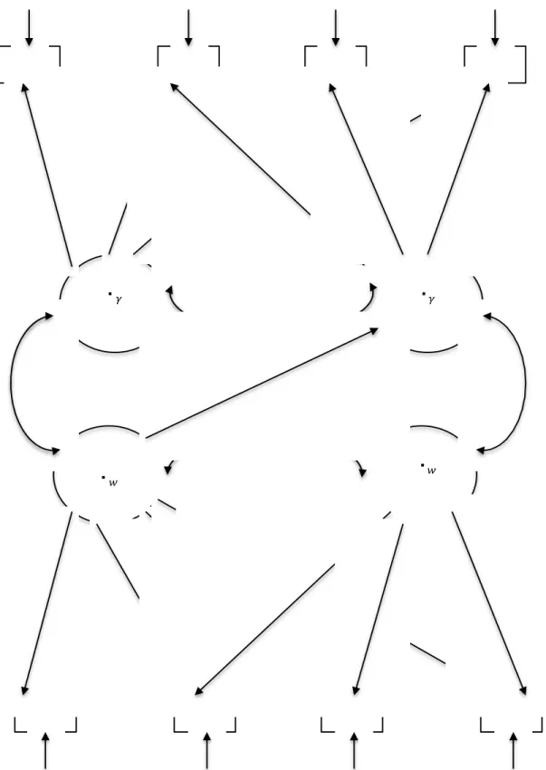
Figure 1. Diagram of a Multivariate Latent Growth Curve Model
�1 �2 �3 �4
�
�
�
�