MOCCA-SURVEY database I. Accreting white dwarf binary systems in
globular clusters – I. Cataclysmic variables – present-day population
Diogo Belloni,
1,2‹Mirek Giersz,
1‹Abbas Askar,
1Nathan Leigh
3and Arkadiusz Hypki
41Nicolaus Copernicus Astronomical Centre, Polish Academy of Sciences, ul. Bartycka 18, PL-00-716 Warsaw, Poland 2CAPES Foundation, Ministry of Education of Brazil, DF 70040-020 Brasilia, Brazil
3Department of Astrophysics, American Museum of Natural History, Central Park West and 79th Street, New York, NY 10024, USA 4Leiden Observatory, Leiden University, PO Box 9513, NL-2300 RA Leiden, the Netherlands
Accepted 2016 July 25. Received 2016 July 22; in original form 2016 April 21
A B S T R A C T
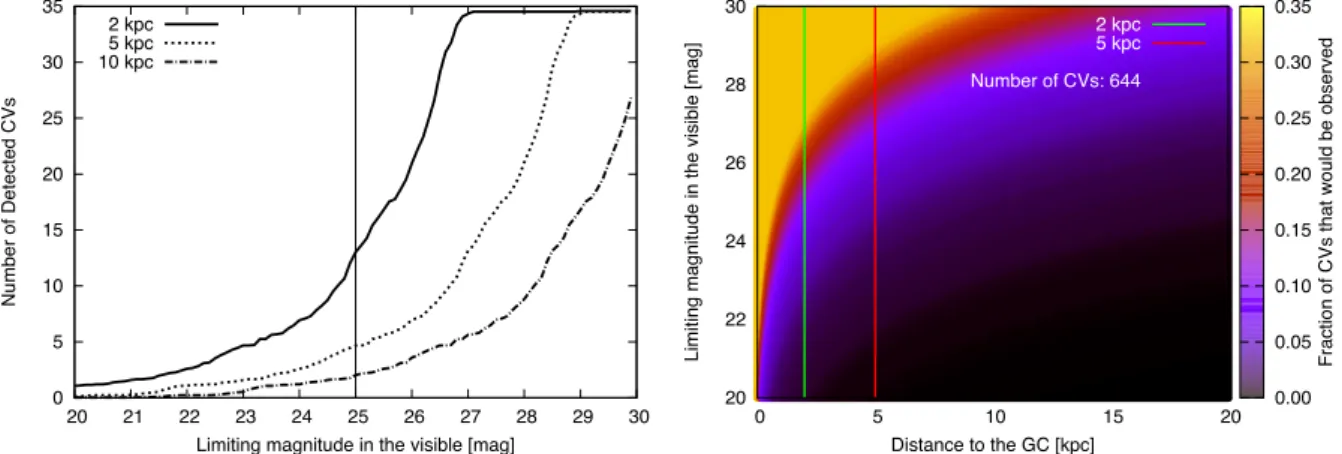
In this paper, which is the first in a series of papers associated with cataclysmic variables and related objects, we introduce theCATUABAcode, a numerical machinery written for analysis of theMOCCAsimulations, and show some first results by investigating the present-day population of cataclysmic variables in globular clusters. Emphasis was given on their properties and the observational selection effects when observing and detecting them. In this work, we analysed in this work six models, including three with Kroupa distributions of the initial binaries. We found that for models with Kroupa initial distributions, considering the standard value of the efficiency of the common envelope phase adopted inBSE, no single cataclysmic variable was formed only via binary stellar evolution, i.e. in order to form them, strong dynamical interactions have to take place. We show and explain why this is inconsistent with observational and theoretical results. Our results indicate that the population of cataclysmic variables in globular clusters is, mainly, in the last stage of their evolution and observational selection effects can drastically change the expected number of observed cataclysmic variables. We show that the probability of observing them during the outbursts is extremely small and conclude that the best way of looking for cataclysmic variables in globular clusters is by searching for variabilities during quiescence, instead of during outbursts. For that, one would need a very deep observation which could reach magnitudes27 mag. Finally, we argue that cataclysmic variables in globular clusters are not necessarily magnetic.
Key words: methods: numerical – novae, cataclysmic variables – globular clusters: general.
1 I N T R O D U C T I O N
The study of star clusters plays an important role in our understand-ing of the Universe since these systems are natural laboratories for testing theories of stellar dynamics and evolution. Particularly, globular clusters (GCs) are one of the most important objects for studying the formation and the physical nature of exotic objects such as X-ray binaries, degenerate binaries, black holes and blue straggler stars, which in turn provides basic information and tools that can help us to understand the formation and evolution processes of star clusters, galaxies and, in general, the young Universe.
Among the most interesting objects in GCs are the cataclysmic variables (CVs) that are interacting binaries composed of a white dwarf (WD) that accretes matter stably from a main-sequence (MS) star – or, in the last stage of their evolution, a brown dwarf (BD;
E-mail:[email protected](DB);[email protected](MG)
e.g. Knigge, Baraffe & Patterson2011, for a comprehensive review). CVs are subdivided according to their photometric behaviour as well as the magnetic field strength of the WD, being, mainly, magnetic CVs (where the accretion is partially or directly via magnetic field lines) and non-magnetic CVs (where the accretion is via an accretion disc). Among the non-magnetic CVs, the most prominent subgroup is that composed of dwarf novae (DNe) which exhibit repetitive outbursts due to the thermal instability in the accretion disc (e.g. Lasota2001, for a review).
1.1 CV formation
CVs are believed to form from an MS–MS binary that undergoes a common envelope phase (CEP) when the more massive MS evolves to a giant (Paczynski1976). In such CEP, the dense stellar giant core and the MS spiral towards each other with the expansion and loss of the common envelope. Most of the angular momentum is lost with the envelope which leads to an orbital period orders of magnitude
shorter (e.g. Webbink1984). After the CEP, a pre-CV is formed in a detached WD–MS binary. Because of angular momentum loss (see below), the separation between the stars decreases up to the formation of the CV, when the MS starts filling its Roche lobe.
In order to form a CV through the above-mentioned scenario, the initial MS–MS binary should approximately have the following properties: (i) the more massive star has M 10 M; (ii) the less massive star is a low-mass MS; (iii) the mass ratio is0.25; (iv) the separation has to be sufficient to allow the pri-mary to expand to a point where it could form a degenerate core (pre-WD) and to permit the contact (the CEP).
The reasons for these conditions come almost naturally. The mass of the more massive star has to be in the acceptable range to form a WD. This justifies the first condition. Besides, the mass ratio after the CEP has to be1 (e.g. Hellier2001). Otherwise, the mass transfer would be unstable and such instability would precipitate further mass transfer and then a merger would occur. This is because the mass transfer rate becomes very large and the WD cannot steadily burn the accreted material, then it swells up to become a giant, producing a common envelope binary and a merger of the stars. The WD mass cannot be greater than∼1.44 M; thus, in order to have the mass ratio less than one, the secondary mass cannot be larger than the WD mass, after the CEP. This justifies the second condition. About the mass ratio, if the initial mass ratio is great (q∼1), then both stars will have similar evolutionary time-scales. In this way, the stars would become WDs at roughly the same time. For a CV however, one star has to be a WD and the other one an MS. This explains the reason for the third condition. Finally, if the separation was too large, the more massive star could not fill its Roche lobe. While if it was too small, the Roche lobe overfilling could lead to a merger. Then, the separation has to be ideal to allow for both the formation of a WD-like core and the close post-common envelope binary.
1.2 CV evolution
Non-magnetic CVs are usually separated in the following way, with respect to the orbital period: (i) if the donor is an MS andPorb
3 h, then it is called a long-period CV; (ii) if the donor is an MS andPmin Porb 2 h, then it is called a short-period CV; and
(iii) if the donor is a BD, it is called a period bouncer CV (in this case,PorbPmin). Besides, in CVs (especially non-magnetic ones),
angular momentum loss is the driving mechanism for their long-term evolution. In the so-called standard model of CV evolution, the dominant angular momentum loss mechanism in long-period CVs is magnetic braking (Rappaport, Joss & Webbink1982), whereas in short-period and period bouncer CVs the driving mechanism is associated with the emission of gravitational radiation (Paczy´nski
1967).
Basically, two important features observed in non-magnetic CVs need to be explained by the standard model. First, the absence of systems in the range of 2 hPorb3 h, known as the period gap
(e.g. Zorotovic et al.2016, and references therein) and, secondly, the existence of a period minimumPmin≈82 min (e.g. G¨ansicke et al. 2009). The standard model reasonably fulfils its role in explaining the observational properties of the CVs.
Briefly, the standard model can be summarized as follows: af-ter the birth of the CV, it will evolve towards short periods due to angular momentum loss. When it reachesPorb ∼ 3 h (upper
edge of the period gap), the donor becomes fully convective and Rappaport, Verbunt & Joss (1983) proposed that at this point the magnetic braking turns off or becomes less efficient (disrupted
mag-netic braking scenario). This results in a decrease of the mass trans-fer rate, which allows the donor star to reestablish its equilibrium and to stop filling its Roche lobe. Then, the system becomes detached since the mass transfer stops. However, such a detached WD–MS binary keeps evolving towards shorter periods due to gravitational radiation. WhenPorb∼2 h (inner edge of the period gap), the Roche
lobe has shrunk enough to restart mass transfer and the system be-comes a CV again. After that, at some point during its evolution (Porb∼ Pmin), the mass-loss rate from the secondary drives it
in-creasingly out of thermal equilibrium until the thermal time-scale exceeds the mass-loss time-scale and it expands in response to the mass-loss, thus, increasingPorb. Consequently, a large number of
CVs are expected to be near the period minimum (known as the period spike) or be in post-period minimum phase – indeed, the abundance ratio for long-period CVs, short-period CVs and period bouncers, respectively, is roughly 1:30:70 (e.g. Howell, Rappaport & Politano1997).
1.3 CV observation
Since the birth of interest in CVs (e.g. Warner1995, for a historical review), several breakthroughs have been taking place in the field, especially due to the Sloan Digital Sky Survey which has provided a reasonable sample that reaches deeper magnitudes and which is capable of recognizing very faint CVs near and beyond the period minimum (Pmin). Such breakthroughs include the confirmation of
the disrupted angular momentum loss at the period gap (Zorotovic et al.2016), the discovery of period bouncers with BD donors (Lit-tlefair et al.2006), the discovery of the period spike aroundPmin
(G¨ansicke et al.2009), among others. They allowed the community to considerably improve the observational data to confront theoret-ical predictions which, in turn, have led to a stronger corroboration between theory and observation.
All the previous discussions, theoretical and observational, are mainly concerned with CVs in the field. For CVs in GCs, the same is not always true because of the influence of dynamical interactions, the ages and distances of the GCs, and the corresponding observa-tional selection effects. Some observaobserva-tional efforts have also been made regarding CVs in GCs, especially a search for an optical counterpart ofChandraX-ray observations (e.g. Knigge2012, for a review on CVs in GCs).
In general, there are four main approaches that have been used for detecting CVs in GCs. In what follows, we will describe them briefly including also the few important works associated with them.
1.3.1 Variability during outbursts
In all possible sorts of variability related to CVs, the most explored is that regarding the DN outbursts which last from days to tens of days and result in an increase of luminosity by roughly 2–5 mag.
The first major investigation of CVs in GCs was done by Shara et al. (1996), who analysed 12 epochs ofHubble Space Telescope
Some comments are needed at this point. As Knigge (2012, see section 5.5) has already pointed out, both Shara et al. (1996) and Pietrukowicz et al. (2008) concluded that DNe are rare in GCs based on the properties of observed CVs in the Galactic field, which seems to be a biased sample of the real population of CVs in the field. If most CVs in the field are, in fact, period bouncers, then the observed CV population in the field (especially the bright ones) is not representative of the real population of CVs in the Galactic field. This is mainly due to the very small duty cycle (fraction of the DN cycle that a DN is in outburst) associated with period bouncers. Hence, in this case, most CVs in the field are unobservable at any given time, and a significant population of hidden CVs exists. Thus, the conclusion that DNe are rare in GCs is not necessarily correct, since it could just be that they are hard and/or unlikely to observe, since there are more period bouncer CVs than originally expected (Knigge2012).
Therefore, it turns out that identifying CVs through their variabil-ity during outbursts is unlikely to reveal the intrinsic population of CVs in GCs since one should be very lucky to detect the outbursts in a sequence of epochs fromHST, given the extremely small duty cycle associated with the CVs in GCs.
1.3.2 Hαimaging
Another possible way to detect CV candidates is using Hαimaging (e.g. Cool et al.1995), since systems that exhibit an excess in Hα show evidence of variability. This technique is generally used to study the counterparts of X-ray sources and has revealed few CVs in some GCs (e.g. Grindlay2006; Pietrukowicz2009). However, doubt remains about the deepness of observations using these techniques, i.e. if they are able to detect the faint population of CVs in GCs.
So far, Cohn et al. (2010) have reached magnitudes as deep as 28 for Hαand 26 from optical observations of theHST. Their study seems to be the least affected by this kind of bias and will be used in this paper as the object for comparison with our results.
1.3.3 FUV band with HST
Another way to detect potential CVs is through their colours. CVs tend to be bluer due to accretion processes. In fact, the energy released from this mechanism makes the region close to the WD hotter, which in turn makes the CVs bluer than typical stars in GCs. This implies that looking for them in the far-ultraviolet (FUV) band withHSTis a good way to find CV candidates (e.g. Dieball et al.2010). Especially because most MSs in GCs emit in infrared which nulls the problem with crowding.
Dieball et al. (2010) carried out a detailed search in the core of M80 and found few candidates. However, due to their limiting magnitude, they could only detect bright CV candidates. In this way, the detection of the faint CVs using theHST’s FUV detectors might also be problematic.
1.3.4 X-rays
The high resolution that has been achieved withChandraallows us to, in fact, reach binaries with compact objects in GCs, especially in their cores.
With regard to CVs, many GCs have been studied withChandra
down to∼1032erg s−1(e.g. Pooley2010). Additionally, the
identi-fication of optical counterparts with deepHSTimaging has allowed for the recognition of many CV candidates (e.g. Bassa et al.2004; Cohn et al.2010; Huang et al.2010), although the number of such
candidates is far from the predicted number of CVs in the observed clusters.
Finally, it is valid to note that below∼1032erg s−1, a large
frac-tion of X-ray sources do not have secure optical counterparts. Below this value, the sources can be chromospherically active binaries (or near-contact binaries of MSs), CVs, foreground and background objects, quiescent low-mass X-ray binaries, millisecond pulsars or black hole X-ray binaries. Any conclusions drawn from a com-parison between the results of our simulations and observations of CVs with small X-ray luminosities should be taken with a grain of salt. This is because the observational sample can be regarded as something of an upper limit, due to an increased probability of contamination from active binaries, chromospherically active stars, accreting neutron stars and black holes, etc.
1.3.5 Classical novae
On the subject of classical novae (CVs with high mass transfer rates and stable and hot discs), it is worth mentioning some observational evidence of different nova rates with respect to the Galactic field.
Curtin et al. (2015) detected novae in a survey of GCs in three Virgo elliptical galaxies (M87, M49 and M84). Such a survey should not detect any novae if there were no enhancement of the nova rate due to dynamics.
A similar result was reached by Shara et al. (2004) while investi-gating one GC of M87. They concluded that classical nova eruptions in GCs are up to 100 times more common than current detections in the Milky Way suggest.
This implies that dynamics are extremely important in enhancing the detection rate of novae in GCs.
1.3.6 What is the lesson from the observations?
Given the crowding of GCs and the faintness of the intrinsic popula-tion of CVs, confirming spectroscopically the many CV candidates that have been observed as real CVs is challenging (e.g. Knigge et al.2003; Thomson et al.2012). On the other hand, the usage of a combination of different techniques (Hαand FUV imaging, X-ray, colour, etc.) can provide almost guarantees the confirmation of CVs, especially for DNe. For instance, Cohn et al. (2010) used Hαimaging and colours to infer that someChandraX-ray sources are CVs.
As it seems, a combination of techniques can provide us with the potential number of CVs in GCs. The only problem is whether or not we can reach faint CVs, given the observational limitations and biases of each technique when combined together.
This indicates that the biases and observational limitations can lead us to incorrect impressions about the nature of CVs in GCs.
1.4 Nature of CVs in GCs
In the most recent survey-like search for DNe, Pietrukowicz et al. (2008) conclude that ‘ordinary DNe are indeed very rare in GC’. Then, either the predicted number of CVs is not correct or the predicted CVs would be non-DNe. Nevertheless, such observational findings do not corroborate theoretical predictions.
typical massive GC. Besides, such CVs would have different prop-erties from the CVs in the field. For example, only∼25 per cent of CVs were formed in binaries that would become CVs in the field. Also, approximately 60 per cent of the CVs did not form via a CEP. This corresponds to a rather strong inconsistency between theory and observation, and the most popular hypothesis that attempts to explain the so-called absence of DNe in GCs is based on the mass transfer rate and the WD magnetic field. Dobrotka, Lasota & Menou (2006) proposed, using the disc instability model (DIM), that a low mass transfer rate combined with a moderately strong WD magnetic field can disrupt the inner part of the disc, preventing, in turn, an outburst in such CVs.
In the mid-1990s, the community started to think that CVs in GCs tend to be magnetic due to the work by Grindlay et al. (1995) who analysed three CVs in NGC 6397 and found the existence of HeIIline in such CVs. Also, Edmonds et al. (2003a,b) argued in the
same direction in their studies of 47 Tuc.
The big problem with this argument is that not only magnetic CVs exhibit the HeIIline in their spectra, but also other types of
CVs (Knigge2012). For instance, Shara et al. (2005) found DN-like eruptions in CV2 and CV3 in NGC 6397 which exhibited helium emission in their spectra. Therefore, it seems that such evidence is not strong enough to claim that CVs in GCs are, principally, magnetic ones.
The main reason for this suspicion is the attempt to explain the discrepancies between observed CVs in GCs and those in the field. This is because a WD magnetic field can prevent instability in the disc and, in turn, suppress the occurrence of outbursts (Dobrotka et al.2006). Besides, it could explain to some extent the unique X-ray and optical properties found for the CVs in GCs.
However, the CV samples in GCs tend to be X-ray selected (Heinke et al.2008) which, in turn, favours the detection of mag-netic CVs (brighter in X-ray than the non-magmag-netic counterpart). Unfortunately, few investigations went deep enough to detect the non-magnetic CVs (1030erg s−1) in the X-ray, and more efforts
should be put in this direction.
Another point in favour of the idea that CVs in GCs are magnetic comes from the fact that magnetic CVs are usually associated with massive WDs (Ivanova et al.2006). In fact, in GCs, the dynamically formed CVs tend to have higher WD masses which, in turn, favours the hypothesis of magnetic CVs.
Above all, such a hypothesis is not well established and can be contested. As has already been mentioned, most CVs should be DNe (Knigge et al.2011). Besides, not only magnetic CVs produce the above-mentioned HeIIemission. Over and above, many optical
counterparts of X-ray sources have been recognized as reasonable CV candidates in some GCs (e.g. Cohn et al.2010), although such numbers are still far from the predicted number of CVs.
1.5 Structure of the paper
From the last subsection, we can say that the ‘CV problem in GCs’ is not yet well understood and solved. In order to contribute to such a discussion, this is the first paper of a series that concentrates on CVs and related objects (such as AM CVn and symbiotic stars) in evolving GCs that attempt to correlate CV properties (and also AM CVn and symbiotic star properties) with cluster initial and present-day parameters.
The main objective of this first paper is to introduce theCATUABA
code (Section 3) that will be used in this series of papers to derive properties of CVs and related objects fromMOCCAsimulations. In
order to test its efficiency and coherence, we concentrate on only six
models with different initial conditions and different properties at the present day (described in Section 4). The models were simulated by theMOCCAcode (Section 2) that simulates real GCs on a
time-scale of one day. Its speed allows for the simulation of hundreds of models in a short time and, in turn, permits a very detailed statistical analysis of particular objects (like CVs) and their correlations with the cluster parameters. The aim of this series of papers is to analyse
theMOCCAdata base with respect to CVs and related objects.
For convenience, we decided to separate the results of this initial work into two separate papers. In this paper, we will concentrate mainly on the present-day (considered here as 12 Gyr) population of CVs present in the analysed models. In the next, we will discuss mainly the CV progenitors and the main formation channels as well as their properties at the moment they are formed and the subsequent evolution up to present day. We will also deal with more general issues like unstable systems, escaping binaries that become CVs, and so on.
In Section 2, we describe theMOCCAandBSEcodes. We also make
some comments with regard to the comparison betweenMOCCAand N-body codes. We describe theCATUABAcode in Section 3, and end
the section by summarizing its main features. The models used in this first work will be described in Section 4, and in Section 5, the main results of the preliminary investigation are presented. We show results associated with the clusters and their present-day populations (PDPs) of CVs as well as results related to observational selection effects when searching for CVs in GCs. We also address some connections between our results and observations and, also, between our investigation and previous studies. We conclude and discuss the main implications of these first results in Section 6. Finally, throughout this paper, we use some new abbreviations, and for convenience, in Appendix A, we clearly define all abbreviations in order to allow the reader to consult them if necessary.
2 M O C C A C O D E
In this section, we describe theMOCCAcode that was used to simulate
the cluster evolution. We also describe theBSEcode that is utilized
byMOCCAto perform the stellar evolution. We end this section by
briefly comparingMOCCA’s performance with that ofN-body codes.
TheMOCCAcode (Hypki & Giersz2013; Giersz et al.2013, and
references therein) is based on the orbit-averaged Monte Carlo tech-nique for cluster evolution developed by H´enon (1971), which was further improved by Stod´ołkiewicz (1986). It also includes theFEW -BODYcode, developed by Fregeau et al. (2004), to perform numerical
scattering experiments of gravitational interactions. To model the Galactic potential,MOCCAassumes a point mass with total mass
equal to the enclosed Galaxy mass at the Galactocentric radius. The description of escape/capture processes in tidally limited clusters follows the procedure derived by Fukushige & Heggie (2000). The stellar evolution is implemented via theSSEcode developed by
Hur-ley, Pols & Tout (2000) for single stars and theBSEcode developed
by Hurley, Tout & Pols (2002) for binary evolution.
2.1 BSEcode
The most important part ofMOCCAwith regard to CVs and related
objects is theBSE code (Hurley et al.2002).BSEmodels angular
are implemented inBSE. The overall CV evolution can be recovered
byBSE, although some comments are necessary here.
With respect to the CEP,BSEassumes that the common
enve-lope binding energy is that of the giant(s) enveenve-lope involved in the process. In order to reconcile the prescription developed by Iben & Livio (1993), we use the recommended value for the CEP efficiency which is 3.0. This is greater than the usually adopted values, but we kept it for the initial investigation.
With respect to CV evolution, the donor radii for long-period CVs are not increased inBSE. There is observational evidence of
an increase in the radii of CV donors with radiative cores (Knigge et al.2011, see their fig. 6). Besides, the mass transfer rate is not adjusted to be in agreement with those derived from observations in the field. This implies a different CV evolution, which leads to the absence of the period gap and to a different period minimum. Additionally, for period bouncers, the mass–radius relation leads to a faster increase in the period after the period minimum.
Even though some efforts should be put into the improvement ofBSEin this direction, for the purposes of this work, the approach
already implemented inBSEseems reasonable. Furthermore, we use
standard values for all parameters in theBSE code (Hurley et al. 2002) None the less, we have to bear in mind these factors while analysing the results.
2.2 Comparison withN-body codes
MOCCAwas extensively tested againstN-body codes. For instance,
Giersz et al. (2013) concluded thatMOCCAis capable of
reproduc-ingN-body results with reasonable precision, not only for the rate of cluster evolution and the cluster mass distribution, but also for the detailed distributions of mass and binding energy of binaries. Additionally, Wang et al. (2016) also comparedMOCCAwith the state-of-the-artNBODY6++GPUand showed good agreement between
the two codes.
In general, many of the simplifying assumptions adopted in the Monte Carlo method that would be naturally accounted for in an
N-body code are unimportant in the regime of cluster masses where Monte Carlo models are ideally suited. For example, Monte Carlo methods treat both binary evolution and direct single–binary and binary–binary encounters as isolated processes, with no chance of being interrupted due to a dynamical encounter. This was recently shown to be a valid assumption in clusters more massive than105
M, with the probability of interruption being of the order of a per cent or less (Geller & Leigh2015; Leigh, Geller & Toonen
2016). The approximations underlying the Monte Carlo method are in many ways perfectly suited to model massive cluster evolution, the regime of star cluster evolution whereN-body models cannot typically go (at least not without being severely limited by the computational expense).
In essence,MOCCAis ideal for performing big surveys and for
carrying out detailed studies of different types of objects like CVs (this paper), blue straggler stars (Hypki & Giersz2013,2016a,b), intermediate-mass black holes (Giersz et al.2015), X-ray binaries, etc., and provides good agreement withN-body codes.
2.3 WhyMOCCA?
TheMOCCAcode has been developed for more than 20 years (Giersz
1998,2001,2006; Giersz, Heggie & Hurley2008), and its current version (Giersz et al.2013; Hypki & Giersz2013) is characterized
by its high speed, its modularity and its detailed information about each and every object in the system.1
In this way,MOCCAis convenient for two purposes that will help
with the investigation of CVs and related objects in GCs: (i) its high speed allows for generating a big data base covering a huge range in the cluster parameter space and subsequently allows for powerful statistical analysis regarding the cluster parameters and the studied objects; (ii) its list of the most relevant events during the life of each star in the cluster admits a very detailed investigation concerning formation/destruction channels, strength of dynamical interactions, and so on.
To sum up, theMOCCAcode is ideal for performing big surveys
and for carrying out detailed studies of different types of exotic objects like CVs, blue straggler stars, degenerate binaries, etc.
2.4 The MOCCA-SURVEY data base
Askar et al. (2016, see their table 1) describes the set of 1950 GC models (called MOCCA-SURVEY) that were simulated using the
MOCCAcode. The models have quite diverse parameters describing
not only the initial global cluster properties, but also star and binary parameters.
The clusters vary with respect to (i) metallicity: 0.02, 0.006, 0.005, 0.001 and 0.0002; (ii) binary fraction: 0.95, 0.3, 0.1 and 0.05; (iii) King model parameter (W0): 9.0, 6.0 and 3.0; (iv) tidal radius:
120.0, 60.0 and 30.0; (v) cluster concentration as measured by the ratio between tidal and half-mass radii: 50.0, 25.0 and tidally filling; (vi) initial binary properties (period, eccentricity and mass ratio), being the initial mass function (IMF) given by Kroupa (2001); (vii) supernova natal kicks for black holes distributed according to Hobbs et al. (2005) or reduced according to mass fallback description given by Belczynski, Kalogera & Bulik (2002).
Despite the fact that the models in the MOCCA-SURVEY were not selected to match the observed Milky Way GCs, they agree well with the observational properties of the observed GCs (Askar et al. 2016, see their fig. 1). They conclude that the MOCCA-SURVEY cluster models are representative for the Milky Way GC population. The six models discussed in the paper were chosen from the MOCCA-SURVEY data base.
3 C AT UA B A C O D E
In this section, we describe the codeCATUABA2(Code for Analysing
and sTUdying cAtaclysmic variables, symBiotic stars and AM CVns), which is capable of investigating CVs. In future improve-ments, it will be extended to also include symbiotic stars and AM CVn.
First, we describe how theCATUABAcode recognizes the PDP in clusters simulated byMOCCAand also how it separates the CVs
ac-cording to their main formation mechanisms. Secondly, we explain the main physical assumption included in the code to study the observational properties of the PDP of CVs in a simulated cluster. Thirdly, we describe other features included in the code and finish
1The simulations were performed on a PSK cluster at the Nicolaus Coper-nicus Astronomical Centre in Poland.
the section with a summary of its operation based on a flow chart of its prime provisions for the analysis of the CV population.
3.1 CV populations
In this subsection, we describe the three populations used to study the CVs. They correspond to the properties of the same CVs at three different times.
3.1.1 The present-day population
The first step in the construction of an inventory of CVs in a GC is the recognition of their population at the present-day age of such a cluster. This is possible due to recurrent snapshots (around every 200–250 Myr) of the system recorded byMOCCAduring the
simulation. We have chosen a snapshot of the cluster at around 12 Gyr to be the present-day cluster. Then, an extraction of the PDP of CVs is easy, based on the definition given in Section 1.
Once the stars in the PDP of CVs are recognized, a complete study of them is done from the progenitor population (see below) up to the PDP.MOCCAprovides a full history of the dynamical and
physical evolutionary events of all stars in the system (Hypki & Giersz2013, for blue straggler stars) through theMOCCA-MANAGER
code.
3.1.2 The progenitor and formation-age populations
Given a star in the cluster,MOCCA-MANAGERcreates a complete
his-tory of all relevant steps during the life of the star thereof. In this chronological list, all stellar evolution and dynamical events are recorded. Therefore, we can easily get the properties of the pro-genitor population and the formation-age population of CVs in the cluster. The progenitor population is defined here as the popula-tion of all binaries that are progenitors of the PDP of CVs, i.e. the population of CVs at the birth of the cluster.
Now, the formation-age population is the population related to the birth of the CV itself, in the sense that mass transfer starts from MS on to a WD. Obviously, for the formation-age population, the time is not unique as in the progenitor population and the PDP. During the cluster evolution, each CV is formed at a specific time, different from the other ones.
One comment about dynamical exchanges and the progenitor population of CVs is necessary at this point.
First, we define a dynamical exchange (or just exchange) by a process in which a binary has one of its components replaced by another star in a binary–single or a binary–binary interaction. It can happen (and happens) that a CV can be formed due to exchanges, in the sense that both the CV components are not the same as those of the primordial binary.
Secondly, the progenitor population of CVs for the cases with-out exchange is easily determined, since the components of the primordial binary are the same components of the CV. Although the situation is not straightforward when there is exchange in the history of the CV. The initial properties in the case of exchange are obtained by getting the properties of the binary with the smaller period (if the exchange took place in a binary–binary interaction) or the properties of the binary (if the exchange happened in a single– binary interaction). In the case that both components of the CV in the PDP were single stars at the cluster birth, then such CVs are excluded from the progenitor population since there is no initial binary associated. In summary:
(i) if both CV components are the same at the very beginning, then the CV is formed from the primordial binary, i.e. there is no exchange during the binary’s life. Thus, this binary enters into the progenitor population;
(ii) if one CV component comes from one binary and the other one comes from another binary, then the properties of the binary with the smaller size at the beginning is saved in the progenitor population;
(iii) if one CV component comes from a binary and the other one was a single star at the very beginning, then the binary properties are saved in the progenitor population;
(iv) if both CV components come from single stars, then there is no binary at the very beginning associated with the CV. Since the progenitor population is defined for binaries only, we do not include any binary for such a CV in the progenitor population.
It is worthwhile to mention that only a few CVs enter in case (iv) above (<1 per cent for the models investigated here) which, in turn, will not change the conclusion derived from the analysis of the progenitor population (in the second paper).
3.2 Categorization of the present-day CVs
Given the complete history of events during the lives of the CVs in the PDP, an attempt of categorizing them comes naturally. Our choice was to separate them with respect to the importance of the dynamical interactions in their lives. For that, we separate every CV in one of the following groups: (i)Binary stellar evolution group (BSE group): the formation of the CV and its subsequent evolution waswithoutany influence of dynamical interactions. This means that a CV in this group has formed from a binary in the progenitor populationonlythrough binary stellar evolution. (ii)Weak dynami-cal interaction group (WDI group): the CV life was influenced only byweakdynamical interactions, in the sense that the binding energy during such interactions changes by a factor of less than 20 per cent during the evolution of the binary in the progenitor population up to the formation of the CV and subsequently, up to PDP. (iii)Strong dynamical interaction group (SDI group): the formation of the CV was influencedstronglyby dynamical interactions, in the sense that such interactions have significantly changed the evolution of the binary in the progenitor population up to the formation of the CV. After the formation of the CVs in this group, there are no subsequent strong dynamical interactions.
Some comments are worthwhile to mention before proceeding further.
(i) Whether a CV belongs to the WDI group or the SDI group is a priori arbitrary. It is based on the change of energy during the dynamical interactions. The cutoff between a weak dynamical interaction and a strong one is 20 per cent of the initial binding en-ergy. This cutoff is for only one dynamical interaction, and it is an arbitrary value connected to the average energy change according to Spitzer’s formula for equal-mass systems (Spitzer1987). Gener-ally, for weak dynamical interactions, most of the interactions are fly-bys, although they can also be resonant interactions, and for strong dynamical interactions, they can be resonant or exchange interactions. As follows, if a binary undergoes one interaction and the change of its binding energy is less than 20 per cent, this binary was involved in one weak dynamical interaction; otherwise, it was subjected to one strong dynamical interaction. If a binary underwent
strong dynamical interaction in its life, then this binary belongs to the SDI group.
(ii) The WDI group is formed by CVs which had only weak encounters during their lives. However, if the number of these en-counters is high for a CV in this group, their cumulative effect can be strong and the properties of the progenitor binary can be strongly changed during its life. Otherwise, if the cumulative effect of the weak dynamical interactions is not strong, the CV will probably have similar properties to those belonging to the BSE group.
(iii) The SDI group also includes binaries which underwent either exchange or merger.
3.3 CV properties
In this part of the methodology, we provide the main assump-tions related to the CV properties. We state the main theoretical and empirical relations used inCATUABA. With such properties, we
can estimate an upper limit for the probability of observing a CV (Section 3.4).
Once the PDP of the CVs is acquired, we can start to analyse the properties of the population thereof. Fortunately, theBSEcode
inMOCCAis capable of giving basic information about binaries in
snapshots of the cluster, like masses, orbital elements, bolometric luminosities, radii and magnitudes. None the less, in the precise case of CVs,BSEis not able to model the typical behaviours of sub-types of CVs, including DIMs. These processes need to be covered in our analysis.
This is necessary because one of the aims of theCATUABAcode
is to calculate the probability of observing CVs as a function of the GC distance and the optical limiting magnitude. Besides, it is rather important to have a model of how the brightness varies with time for systems that undergo variability (like CVs). In the specific case of CVs, the variability is caused by either eclipses or outbursts, and the chances of detecting a CV depend on how its magnitude varies with time due to either eclipses or recurring outbursts. In order to compute such brightness variations due to outbursts, the well-accepted DIM will be used as it provides maximum values for the CV luminosity during quiescence and during outburst.
3.3.1 CV types
As we have already mentioned, one expects that most CVs are DNe (Knigge et al.2011). In this sense, we should be able to model DNe. DNe are characterized by outbursts due to the thermal instability in the accretion disc (e.g. Smak2001). During the outburst, their luminosity increases by typically 2–5 mag. Also, outbursts last from days to tens of days, and occur every tens of days or even decades. In order to classify a CV as a DN, we adapted equations A.3 and A.4 of Lasota (2001) which defines the limits for the disc stability based on the CV properties, the position inside the disc and the viscosity parameterα. Hence, the mass transfer rate ˙MB defines
the limit between hot/ionized/stable and unstable disc, and the mass transfer rate ˙MAdefines the limit between cold/neutral/stable and
unstable disc. They are
˙
MA = 6.344×10⁻¹¹α−c0.004
MWD
M
−0.88
× r 1010cm
2.65
Myr−1 (1)
and
˙
MB = 1.507×10⁻¹⁰α0h.01
MWD
M
−0.89
× r 1010cm
2.68
Myr−1 (2)
whereMWDis the WD mass,αcis the usual viscosity parameter for
the cold branch of the Shakura & Sunyaev (1973) solution, adopted here as 0.01,αhis the usual viscosity parameter for the hot branch
of the Shakura–Sunyaev solution, set here as 0.1, andris the radial distance from the centre of mass. At eachr, ˙MAis the critical mass
transfer rate below which the disc is cold/neutral and stable and ˙MB
is the critical mass transfer rate above which the disc is hot/ionized and stable.
Both values ( ˙MAand ˙MB) are computed based on analytic fits
concerning 1D time-dependent numerical models of accretion discs, using an adaptive grid technique and an implicit numerical scheme, in which the disc size is allowed to vary with time (Hameury et al.
1998).
Given the mass transfer rate of a CV in the PDP ( ˙Mtr), we have
three different regimes: (i) if ˙Mtr>M˙Beverywhere in the disc, the
disc is stable and hot; (ii) if ˙Mtr<M˙Aeverywhere in the disc, the
disc is stable and cold; (iii) if ˙MA<M˙tr<M˙B, in some ringrof
the disc, the disc is unstable and undergoes repetitive outbursts.
3.3.2 Mass transfer and accretion rates
Before moving on, we have to explain how the mass transfer and accretion rates are calculated, since this information is not given by theBSEcode inMOCCA. Themass transfer ratehere is defined as the
mass-loss rate of the donor, i.e. the rate at which the accretion disc is fed (in the case of a non-magnetic CV or an intermediate polar CV). On the other hand, theaccretion rateis defined as the rate at which the mass flows through the accretion disc towards the WD.
It is worth noticing that in long-period CVs in which the donor is an evolved star (sub-giant), the mass transfer can also be driven by the nuclear expansion of the donor star, e.g. AKO 9 in 47 Tuc (Knigge et al.2003). Nevertheless, based on our definition of CV (Section 1), we are mainly concerned with unevolved donors, which is reasonable, since MS stars are more common in GCs than more evolved donors by orders of magnitude.
On how the mass transfer rate is computed, for simplicity, let us consider only one CV. From the list of all relevant events during the CV life, two quantities are used to compute the mass transfer rate, namely time and donor mass. For each timestep in the CV life, the mass transfer rate is computed based on the amount of mass lost by the donor due to angular momentum loss during this timestep. Thus, the mass transfer rate calculated here corresponds to a crude estimation. The accretion rate will be treated latter in this section.
We assume, a priori, that the disc is not disrupted and the inner edge of the disc is the WD radius. Besides, the outer edge of the disc during outbursts is assumed to be 90 per cent of the WD Roche lobe (Smak1999) which, in turn, is computed based on the equation derived by Eggleton (1983).
With these values for the viscosity parameter and edges of the disc, it is straightforward to distinguish between stable and unstable discs by using equations (1) and (2).
In order to calculate the observational properties of the CVs with unstable discs, we need to find the associated accretion rates ( ˙Md)
through the disc, specifically during outburst ( ˙MdO) and during
TheBSEcode insideMOCCAis capable of giving some information
about the binary itself. Nevertheless, information about the other components (hotspot and disc) for a DN is missing. Therefore, we adopt maximum values for the accretion rate during quiescence and outburst. For the accretion rate during quiescence, we simply assume ˙MdQ=M˙A, while for the outburst, we adopt ˙MdO=M˙(d),
where ˙M(d) is obtained from equation 3.27 of Warner (1995), which is qualitatively similar to the expression derived by Lasota (2001). We choose to use the maximum values during quiescence and during outburst because we are interested in an upper limit for the probability of observing a CV. A similar approach for the accretion rate is used in theSTARTRACKcode (Belczy´nski et al.2008) which
deals with X-ray binaries.
Concerning the disc radius for a DN in quiescence, we adopt a value of 50 per cent of the WD Roche lobe for the outer edge (Harrop-Allin & Warner1996). While for the outburst, as we have already mentioned, we use a value of 90 per cent of the WD Roche lobe (Smak1999).
3.3.3 CV visual luminosity
The WD and donor bolometric luminosities are provided by theBSE
code. We only need additional information about the hotspot and the disc. The bolometric luminosity of the hotspotLbHSis given by
(e.g. Warner1995, p. 83)
LbHS =
f 8
G MWDM˙tr
rd ,
(3)
wheref∼1.0 is an efficiency factor, and the bolometric luminosity of the discLbd is given by (Paczynski & Schwarzenberg-Czerny 1980)
Lbd =
G MWDM˙d
2rd
1−3
RWD
rd
+2
RWD
rd 3
2
(4)
withrdbeing the outer edge of the disc andRWD being the WD
radius.
Once the bolometric luminosities are computed,CATUABA
calcu-lates the bolometric correction for the hotspot and for the disc. The hotspot bolometric correction is computed assuming an ellipsoid, with the semi-axessa=0.043aandsb=0.22sa, whereais the
semi-major axis (Smak1996). Given the shape of the hotspot and using the bolometric correction coefficients given by Torres (2010), the code computes the hotspot temperature and also the visual lu-minosity and magnitude.
A similar procedure is done for the disc, although it is necessary to integrate over the entire spatial extent of the disc. This is done following the procedure by Paczynski & Schwarzenberg-Czerny (1980) and also using the bolometric correction coefficients given by Torres (2010).
3.3.4 CV X-ray luminosity
Another important observational property calculated by theCATUABA
code is the X-ray luminosity. This is computed based on equation 4 derived by Patterson & Raymond (1985), in the band [0.5–10 keV], for a slowly rotating WD:
LX = ε G M WDM˙dQ
2RWD
, (5)
where the factorε=0.5 is the correction for the fraction of the X-rays emitted inwards and absorbed by the WD.
Patterson & Raymond (1985) proposed an explanation for the origin of the X-ray luminosity in CVs. They showed that, at small accretion rates (during quiescence for DNe), the boundary layer (region between the accretion disc and the WD) is the likely site of most of the observed hard X-rays. This is because at small accretion rates the boundary layer is thin. In the case of high accretion rates (during outbursts for DNe), the boundary layer is thick and con-sequently the observed hard X-rays do not come from this region (Eze2015). Actually, one of the open questions on this matter is associated with the origin of the hard X-ray luminosity observed for systems with high accretion rate (Mukai et al.2014). As there is no consensus with respect to systems with high accretion rate, equation (5) is used only for the quiescent stage (for DNe) or for CVs with stable and cold discs. There is no X-ray luminosity for the DNe during outbursts or CVs with stable and hot discs modelled
inCATUABA. That is the why in equation (5) the ˙MdQis given by its
value in the boundary layer, assumed here as being the WD radius.
3.3.5 DN time-scales
Important time-scales for DNe are the recurrence time and the du-ration of the outbursts. The recurrence time can be defined as the interval between two outbursts and is computed here based on the observational fit done by Patterson (2011)
trec = 318
Mdonor/MWD
0.15
−2.63
d, (6)
whereMdonoris the donor mass andMWDis the WD mass. Notice
that the smaller the mass ratio, the longer the recurrence time. The duration of the outburst is the interval between the beginning and the end of the outburst, and we adopt here the observational fit from Smak (1999)
tdur = 2.01 (Porb)0.78 d, (7)
wherePorb is the orbital period. Note that the longer the orbital
period, the longer the duration of the outburst.
3.3.6 CVs with stable discs
Since not all CVs are DNe, theCATUABAcode also has to be able to deal with systems that have stable discs. Now, we describe what happens in these cases. In stable (hot or cold) discs, it happens that the mass transfer rate is identical to the accretion rate. We adopt the maximum values in both cases, again using the prescription given by Lasota (2001) and Warner (1995), i.e. for stable and cold discs, we use ˙MA, and for stable and hot discs, we use ˙M(d). Then, the
same procedure is executed for computing the luminosities and the bolometric correction. Obviously, computations for the recurrence time and duration of the outburst are not necessary.
3.4 Probability of detecting a CV
One of the objectives of this work is to compute the probability of detecting a DN when observing a given GC at a distanceRGC
associated with a given optical limiting magnitudemlim.
For that, let us first consider two principal configurations: (i) the CV can be detected by an optical detector/telescope in quiescence; (ii) the CV can be detected by an optical detector/telescope in outburst.
such a combination. Given a distanceRGCand a limiting magnitude mlim, the probability (Pobs) can simply be taken from the
follow-ing. If the source can be detected only during outburst, thenPobs= PO(tdur,trec)=tdur/trec is the probability of detecting the outburst
in one night3. If the source can be detected during quiescence and
during outburst, thenPobs=Pecl+PO(tdur,trec)=1/3+tdur/trecis
the probability of detecting such a CV, during the eclipse or during outburst, in one perfect night, wherePeclis the probability of a CV
being an eclipsing one. Finally, if the CV cannot be detected even during outburst, then the probability is null.
Notice that we are assuming that the only way to detect a CV during quiescence is when the stars eclipse each other. That is the why we add the 1/3 term in the expression for the probability which corresponds to the probability of a binary being an eclipsing one (e.g. Hurley et al.2002, see appendix A2 for a demonstration).
In summary, we have the following law for the probability of detecting a DN during its cycle:
Pobs = ⎧ ⎪ ⎪ ⎪ ⎪ ⎪ ⎪ ⎪ ⎪ ⎪ ⎪ ⎪ ⎪ ⎪ ⎪ ⎪ ⎨ ⎪ ⎪ ⎪ ⎪ ⎪ ⎪ ⎪ ⎪ ⎪ ⎪ ⎪ ⎪ ⎪ ⎪ ⎪ ⎩
tdur/trec, if the CV can be
observed only during
outburst
1/3+tdur/trec, if the CV can be
observed during
quiescence
0, otherwise.
(8)
It is worth explaining some issues associated with the probability expressed in equation (8). We are not considering many of the observational difficulties associated with observing a GC, like its intrinsic characteristic of being in a crowded field, a reduced number of (good) nights dedicated to observing the GC thereof, instrumental problems, etc.
Since the probability is computed mainly with the aim of dealing with the apparent absence of DNe in GC, we do not have any prescription forPobsassociated with CVs having stable discs. Thus,
equation (8) is associated with DNe only.
3.5 Additional considerations
So far, we have described the main aspects of the CATUABAcode
used to study the PDP of CVs present in GCs simulated byMOCCA. None the less, other options are available in the code that allow for studying aspects of the CVs not only included in the PDP. Now, we turn to such options.
3.5.1 Destroyed CVs
Throughout the evolution of a GC in theMOCCAcode, not only are
the CVs in the PDP formed, but many other CVs are formed as well. The only difference is that they do not survive up to the present day. One of the capabilities of theCATUABAcode is the ability to collect
relevant information about such systems, in order to investigate their properties and the reasons for their absence in the PDP.
This option gives similar information as given by the study of the PDP. The main difference is that the information regarding the
3The quantityt
dur/treccorresponds to the very DN duty cycle.
PDP is replaced by the information associated with the destruction-age population which correspond to the CV properties immediately before their disappearance from the cluster.
With such a sample, one can investigate the properties of such ‘destroyed’4CVs and also delineate general destruction channels.
In the possession of such information, we can separate the CVs into groups, according to the main channels of ‘destruction’ (sim-ilarly to what is done for the CVs in the PDP). Our choice on the matter is as follows. (i)Destruction due to binary stellar evolu-tion group: the CV stops being a CV due to some evolutionary process and without any influence from dynamical interactions. (ii)Destruction due to escape: the CV life in the cluster is interrupted because the CV escaped the cluster while still being (or not) a CV af-ter the escape. (iii)Destruction due to dynamical interaction group: the death of the CV was caused by a dynamical interaction, but the outcome of this interaction remains in the cluster.
Notice that a CV can escape from the system due to either re-laxation processes or dynamical interactions. Both cases here are related to the destruction due to escape group. In the case associated with CVs destroyed by dynamical interactions without escaping, such CVs belong to the destruction due to dynamical interaction group.
3.5.2 Field-like CVs
Two other important tools in the code are the possibility to run the BSE code alone for the initial binaries and for the escaping
binaries. The former allows one to study the field-like population (without dynamics) of CVs that comes from the initial binaries. This permits one to investigate how different the cluster and field-like populations are, or even constrain the initial distributions of binaries with available data from observed CVs in the solar neighbourhood. The latter allows the study of the escaping CV evolution and the evolution of escaping binaries that will become CVs up to 12 Gyr.
Again, for theBSEruns, similar information is recorded about
pro-genitor population, formation-age population, PDP and destruction-age population. In the case whenBSEevolves the initial binaries,
information about the progenitor population, formation-age pop-ulation and PDP is saved for the CVs that survive up to 12 Gyr. If the CV is somehow ‘destroyed’, then the information about the destruction-age population is saved instead of the information about the PDP. WhenBSEis run for the escaping binaries, additional infor-mation is saved for the binaries immediately after the escape. This would correspond to the escaping-age population. Again, informa-tion about the formainforma-tion-age populainforma-tion is saved always and, about destruction-age population or PDP, whether or not the CV survives up to 12 Gyr.
3.5.3 Time dependence of CV properties
The last resource provided by theCATUABAcode in its current version is the possibility to investigate the time-dependent properties of the CVs from the cluster birth up to the present day. Such an option in the code utilizes the cluster snapshots. For a particular snapshot, all CVs present in it are collected and their semi-major axis, period,
mass ratio and mass distributions are generated. This is done for all the snapshots of the cluster (every 200–250 Myr, depending on the cluster). It provides an efficient way to investigate how such distributions evolve with time. Apart from the distributions, the code also saves the average and median values of the semi-major axis, period, mass ratio and masses through time, again, based on all snapshots.
This option is available for theMOCCAsnapshots and also for the
BSEsnapshots, when one is interested in comparing both populations
of CVs. In this case, the timesteps for generating the snapshots of the cluster inMOCCAandBSEhave to be the same. In the case when
onlyBSEsnapshots are being analysed, the timestep for the creation
of such snapshots can be any value. The timestep associated with
MOCCAsnapshots is defined before the simulation, and this value has
to be used in theCATUABAcode.
Here, we summarize all the possible ways of using theCATUABA
code as described above.
3.6 Summary ofCATUABAfeatures
In order to account for the limitations of the above-presented ap-proach, we present a summary it and address the principal hypoth-esis which should be kept in mind when interpreting the results presented in this series of papers (especially, in Section 5.5 of this paper). The study of the CVs is carried out in the following way.
(i) The first step is to recognize the PDP of the CVs in the snap-shot of the cluster at 12 Gyr. The next is to compile the most relevant events in the history of all the stars in the PDP. With this, we can un-equivocally separate the CVs into three groups, namely BSE group, WDI group and SDI group.
(ii) The second step is to cover the shortcomings for CVs with stable or unstable discs. This is done by considering the formalism in the DIM. Suchmodus operandiprovides good agreement with observation, and also allows for filling the deficiencies left byBSE.
(iii) The third step is to compute two important time-scales of DNe, namely recurrence time and duration of the outburst. This is done by using empirical relations.
(iv) The fourth step is to calculate the probability of observing and detecting the DNe by means of equation (8).
It is rather important to mention at this point that we do not have any prescription for magnetic CVs. They correspond to roughly 25 per cent of CVs in the field (e.g. Wickramasinghe & Ferrario
2000; Ferrario, de Martino & G¨ansicke2015) and can be extremely important in GCs (e.g. Grindlay et al.1995; Dobrotka et al.2006; Ivanova et al.2006).
Secondly, most short-period DNe are SU UMa stars which also have superoutbursts in addition to normal outbursts. Superoutbursts are more luminous (increase in brightness by∼1 mag), last longer (10–20 d), and are more infrequent (every 3–10 DN cycles). In this way, the chances to observe a short-period DN during superout-burst are even smaller since for one superoutsuperout-burst, we have 3–10 outbursts. Since we are interested here in the upper limit of the probability, we neglect this complication.
Thirdly, the values for the accretion rate and, in turn, luminosities and magnitudes, are derived based on maximum values provided by the DIM. Besides, the mass transfer rate computed is a rough estimate since it is based on average value of the donor mass-loss during the CV evolution.
Finally, all information obtained in theCATUABAcode is associated
with theBSEcode. Thus, it is limited by what theBSEcode is capable
of.
To sum up, the principal hypothesis developed in this work in-cludes the neglect of magnetic CVs and superoutbursts for the short-period DNe; the extrapolation of empirical relations for the CVs; the assumption of theoretical maximum values for the accretion rate, and consecutively, maximum luminosities. All these assumptions have the aim of computing the upper limit for observing the CVs.
It is worth noticing that the procedure described above is some-what forged, although reasonable. This is because we cannot retrieve precisely the CV properties from observations.
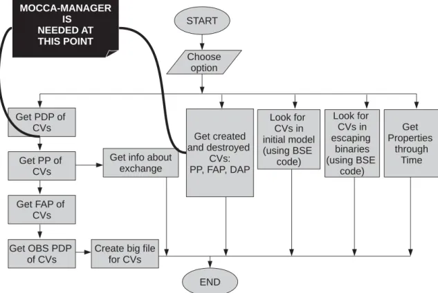
Other options can be used independently from what is done for the CVs in the PDP (Section 3.5). A flow chart of the code is presented in Fig.1. In the very beginning, the user has to choose an option which includes
(i) getting the PDP, the progenitor population, the formation-age population and the observational properties for the CVs present in the cluster at 12 Gyr;
(ii) getting the progenitor population, escaping-age population, formation-age population and destruction-age population for the CVs formed during the cluster evolution but not present in the PDP; (iii) getting the progenitor population, formation-age population and destruction-age population/PDP for the field-like CVs;
(iv) getting the progenitor population, formation-age population and destruction-age population/PDP for the CVs created from es-caping binaries;
(v) getting the distributions of the main orbital elements of the CVs though time.
Notice that this flow chart reflects the underlying coding structure and is not meant to represent a logical flow or progression in the data analysis.
After introducing theCATUABAcode and also the hypothesis in it,
we are able to turn to the description of the six models (Section 4) that are used in these initial investigations and the main results on the PDP of CVs in such models (Section 5).
4 M O D E L S
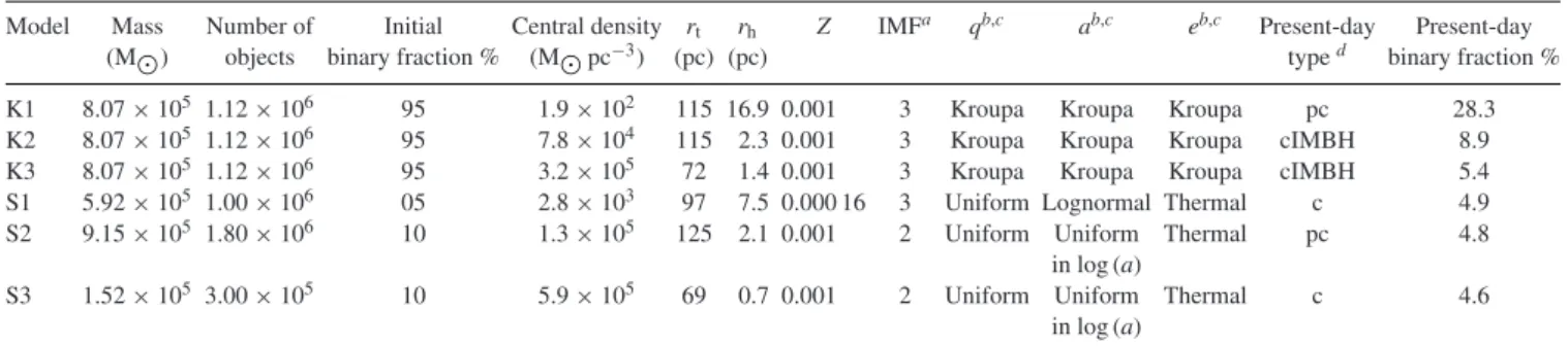
In this first examination of CVs in GCs, we have chosen six models that differ mainly with respect to the initial central density, initial binary distributions and initial binary fraction. The restricted num-ber of models used in this work is due to its very objective nature: to construct the numerical apparatus used to study CVs based on
MOCCAsimulations, to check its consistencies and to gain experience
for data analysis.
Before proceeding further, it is convenient to define the initial binary population (IBP) since it is a rather important concept in this work. The initial binaries in GCs follow determined distributions for their parameters: semi-major axis, eccentricity, masses, mass ratio and period. Hereafter, the initial binaries associated with the initial distributions for their parameters belong to the IBP. In other words, the IBP is the group that contains all initial binaries, in a given initial cluster, associated with specific initial distributions for their parameters. In this work, we analyse models with two distinct IBPs.
The first set of models, defined as the K models, corresponds to models constructed based on the IBP derived by Kroupa (1995,
Figure 1. Flow chart of theCATUABAcode. Notice that to get the info about progenitor population and formation-age population, for CVs present (or not) in the cluster at 12 Gyr, the files containing the very detailed history of the stars lives are needed. This is obtained by using theMOCCA-MANAGERcode. Notice that this flow chart reflects the underlying coding structure and is not meant to represent a logical flow or progression in the data analysis.
primordial binaries,5the same initial mass 8.07×10⁵M
and the same initial number of objects (binaries and single stars) 1.12×10⁶.
But they differ with respect to the initial central density, having, in Mpc−3, 1.9×10², 7.8×10⁴and 3.2×10⁵. Thus, we have one
sparse model, one dense model and one very dense model. The other set of models, defined as S models, follows the ‘Stan-dard’ IBP and has low binary fractions of 5 and 10 per cent. The Standard IBP is associated with a uniform distribution for the mass ratio, a uniform log or lognormal distribution for the semi-major axis and a thermal distribution for the eccentricity. As in the K models, we have chosen models with different initial central den-sities, namely 2.8×10³, 1.3×10⁵and 5.9×10⁵, in M
pc−3.
Again, for the set of S models, we have a sparse model, a dense model and a very dense model. Differently from the K models, in the S models, we have different initial numbers of objects and initial masses.
We have used two IMFs that follow the broken power law ξ(m)∝m−α, defined by Kroupa et al. (1991, 1993). The IMF2 (canonical) is such that it hasα=1.3 for 0.08≤m/M ≤0.5 andα=2.3 for 0.5≤m/M ≤mmax/M(Kroupa2008). The
IMF3 (multiple power law) is such that it hasα=1.3 for 0.08≤
m/M ≤0.5,α=2.3 for 0.5≤m/M ≤1.0 andα=2.7 for 1.0≤m/M ≤mmax/M(Kroupa2008). The star mass in this
study lies between 0.08 and 100 M.
We assume that all stars are on the zero-age main sequence when the simulation begins and that any residual gas from the star
5We set the initial binary fraction for the models with Kroupa IBP different from 100 per cent in order to avoid computational problems that arise in MOCCAif there is no single star in the initial model.
formation process has already been removed from the cluster. Ad-ditionally, all models have low metallicity, are initially at virial equilibrium and have neither rotation nor mass segregation. More-over, all models are evolved for 12 Gyr which is associated with the present day in this investigation.
In Table 1, we summarize the main parameters of the initial models.
In addition to the evolution done using MOCCA, we have also
evolved the initial models (actually, the IBP) withBSEalone during
12 Gyr. In such a way, we will have information not only about the cluster CVs but also on the field-like CVs. This will help us to compare both groups of CVs that come from the six initial models.
5 R E S U LT S A N D D I S C U S S I O N
In this section, we present the main results related to the PDP of CVs in the six models described in Section 4. First, we will discuss some evolutionary properties of the models. Secondly, we will state the properties of the PDP of CVs. After that, we will show how observational selection effects can hide the CV population in observed GCs by computing the upper limit of observing such CVs. We also address some discussions on the main points and correlate this work with previous ones. Finally, we discuss possible observational procedures that might help in detecting the missing DN population.
5.1 Cluster evolution